Assessment of different simplified resist models

HAL Id: hal-00022164

https://hal.archives-ouvertes.fr/hal-00022164

HAL is a multi-disciplinary open access archive for the deposit and dissemination of sci-entific research documents, whether they are pub-lished or not. The documents may come from teaching and research institutions in France or abroad, or from public or private research centers.

L’archive ouverte pluridisciplinaire HAL, est destinée au dépôt et à la diffusion de documents scientifiques de niveau recherche, publiés ou non, émanant des établissements d’enseignement et de recherche français ou étrangers, des laboratoires publics ou privés.

Assessment of different simplified resist models

David Fuard, Maxime Besacier, Patrick Schiavone

To cite this version:

David Fuard, Maxime Besacier, Patrick Schiavone. Assessment of different simplified resist models. 2002, pp.1266-1277. �hal-00022164�

Assessment of different simplified resist models

D. Fuard, M. Besacier, P. Schiavone, (Laboratoire des Technologies de la Microélectronique,

CNRS, c/o CEA Grenoble, 17 rue des Martyrs 38054 GRENOBLE cedex 9 France)

ABSTRACT

Resist modeling is an attractive way to predict the critical dimensions of patterned features after lithographic processing. Unfortunately, previous works have shown that model parameters are very difficult to determine and have

often a poor range of validity outside the dataset that have been used to generate them [1, 2].

The goal of this work is to assess different simplified resist models using a systematic method. We have studied the accuracy of aerial image model and aerial image plus gaussian noise convolution model. The approach is based on the comparison between simulated and experimental data for periodic lines of various dimensions at various illumination conditions. We also propose a reliable expression for Bossung curves fitting. Using simple physical considerations, the expression has been made very simple and efficient.

After a proper setting of the model parameters to the experimental data, mean CD discrepancies between simulation and experiment are as small as 5% and can be 3% for certain feature types. Moreover, we show that simple gaussian noise convolution models can be predictive with the same accuracy. The method for CD prediction is fully described in this paper.

Significant improvements have been made in resists modeling over the last several years, but simplified resist models such as "aerial image + gaussian noise " seems to be an effective tool for CD prediction, which remains the major demand of IC manufacturers.

1. INTRODUCTION

When setting up new processes, using advanced steppers, resists and a wider range of variables, IC manufacturers increasingly rely on computer simulation programs to support process optimization. The problem of predicting line width of circuit features remains not fully solved. This situation is not surprising, because the modeling of a process has to consider the complex interplay between mask, stepper and resist. There is still no consensus on the modeling of chemically amplified resist and existing models differ in the description of kinetics of the diffusion phenomena during post exposure bake or in the specification of the development rate.

Lithographic models that accurately predict resist performance are invaluable tools for resist design evaluation. However, authors have shown that current chemically amplified resist models derived from fundamental principles

“may exhibit only sporadic success in reproducing experimental data”[1]. Moreover, the optimum performance of a

simulation is only achieved by an appropriate determination of the model parameters and by a careful exploration of

different modeling options [2]. At the moment, these models are very specific, but hardly give reliable predictions on

critical dimensions (CD) of final patterned features simultaneously with accurate resist profiles.

Moreover, the techniques for measurements and parameter extraction are often very delicate, and incorrect input

parameters is another source of simulation to experiment mismatch [3, 4]. Finally, if lithographic simulations consist in

manually changing some parameters in a way that the match between real and simulated data improves, the results can become very subjective.

To ease CD prediction (which is the main demand of IC manufacturers) via simulations, and to avoid the difficult task

of resist parameters extraction associated to full resist models, we prefer the use simplified resist models [1, 5]. Their

advantage is to provide a simulation, with very few parameters compare to full models. Although these models are both quite simple to run and predictive, they suffer several limitations. They are not intended to give insight into fine physical phenomena explanation for the different steps of the resist processing (acid generation reaction and diffusion, polymer deprotection, dissolution rate, developer selectivity, thermal decomposition, PEB acid diffusivity, PEB acid evaporation, etc.) and no prediction of resist profiles is possible. Thus, more sophisticated models for resist modeling remain very important for physical understanding.

The aim of this work is to assess a simple model, which could be predictive for the widest range of feature sizes, pitches and types (lines or contact), and for all wavelengths ranging between 248 and 157 nm.

We investigate, by simple comparison between experimental data and computer simulations using Solid-C [6], the accuracy of the following three simplified resist models. All of them are based on variants of the aerial image associated with a resist threshold model:

- the first model, with the aerial image only

- the second, with the diffused aerial image using fixed gaussian noise convolution

- and finally the third, with the aerial image using variable gaussian noise convolution

This paper presents a procedure for the tuning of the few parameters of these three simplified models. Then, the accuracy of each model is evaluated by direct comparison between experimental and simulated data.

2. EXPERIMENTAL & SIMULATION APPROACH

This section presents the procedure, which has been used to allow the comparison between experimental datasets, expressed as a function of exposure dose and defocus, and simulated datasets, expressed as a function of intensity threshold and defocus.

All the data involved in the present work are based on 193nm resist (0.5µm thick Sumitomo PAR 700). The final features were obtained using conventional illumination and binary masks. The nominal CD of the lines on the mask is 120 nm, with various line to space ratio L/S = 1:1.5, 1:1.75, 1:2, 1:3 and isolated lines. An ASML /900 stepper (0.63

numerical aperture, and partial coherence σ of 0.6 and 0.85) was used for the exposures.

An Hitachi Critical Dimension Scanning Electron Microscope (CD-SEM) was used for evaluating the line CDs of developed resist features. The accuracy assessment of our simplified resist models has been lead using Focus Exposure Matrix (FEM). The simulated data are obtained using Solid C (from Sigma-C Gmbh). No mask correction has been used in the simulations. Experimental conditions are summarized in Table 1.

To compare experimental and simulated FEM datasets, we have to express either experimental FEM as a function of intensity threshold or simulated ones as a function of exposure dose. Finally, the accuracy of each model is evaluated by calculation of the mean of the absolute values of CD difference between experimental and simulated data. An illustration of this methodology is given with more details for the case of the aerial image plus threshold model in section 3.1.

3. MODEL ASSESSMENT

3.1 "Aerial image plus threshold" model

For this first model, the aerial image is used. Simulated FEM datasets are generated. The comparison procedure is achieved by the following procedure (fully described only for this first model).

3.1.1Build-up of a general fitting procedure for experimental & simulated isofocal CD determination

In order to compare experimental and simulated FEM datasets, a fitting procedure is necessary. It allows the determination of a suitable expression of the Bossung curves, and then the direct comparison between experimental and simulated FEM datasets with the same dose set.

In this section, we propose a fitting expression based on physical considerations. This analytical expression of the Bossung curves includes isofocal CD and dose (or threshold for simulated datasets) at isofocal CD as explicit parameters. This will prove in the following to be very helpful.

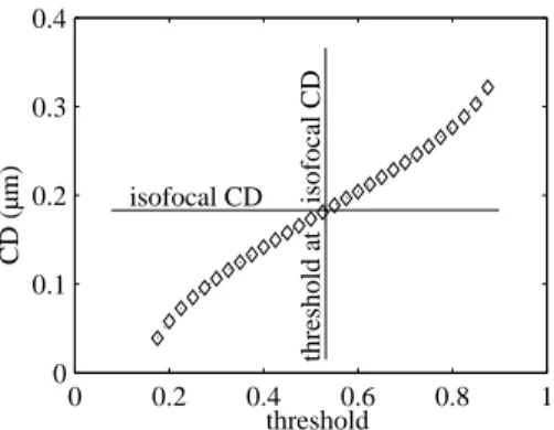
A plot of a FEM for the simulated data expressed as a function of threshold is shown in figure 1. Bossung curves can be

fit by a general polynomial expression as used in the literature [7]:

CD = (a0 + a1.f + a2.f2).(b0 + b1.t + b2.t2) = a00 + a10.f + a01.t + a11.f.t + a20.f² + a02.t² + a21.f²t + a12.ft² + a22.f².t² (1)

where f is the defocus, t is the aerial image intensity often called threshold in the following of the paper. ai, bi, aij are

constants.

With a second power law in threshold and defocus, there is not less than nine terms to be adjusted during the fit. By taking into account simple characteristics of the Bossung curves, this number can be greatly reduced, thus allowing a faster and more reliable convergence of the fitting procedure. Moreover, we try to include as explicit terms of the

expression, much significant physical terms as possible. The first improvement is to replace f and t by (f-f0) and (t-t0) to

gain three physical terms in our Bossung fitting expression: f0 represents the best focus, t0 represents the threshold at

This expression remains too general and several improvements can still be done. Some terms are of no interest in the FEMs fit. Indeed, as shown in figures 2 and 3, the simulated data in threshold exhibit two symmetries, and this can be a useful property to exploit. We identify that the Bossung curves, which are expressed as a function of threshold and defocus, are:

- even functions of defocus for a given threshold as illustrated in figure 2: - odd functions of threshold for a given defocus (cf. figure 3):

So, our fitting expression can become:

CD = c00 + [c1.(f-f0)4 + c2.(f-f0)2 + c3].[d1.(t-t0)5 + d2.(t-t0)] (2)

where ci, di, c00 are constants.

This expression is able to provide a better fit of the simulated data with only five adjustable coefficients. The result is shown in figure 4, the simulated FEM fit is apparently good. But if we enlarge the range of CDs plotted, the fitted function takes a very strange look out of the isofocal CD neighborhood (cf. figure 5). To improve the validity range of

the expression, the implementation of conditions on ci and di coefficients is useful. These conditions are the expression

of physical considerations such as non-crossing Bossung curves [8]. To avoid the Bossung curves crossing, simple

limitations on ci and di coefficients are used. We easily see that ci and dj must be such as ci*dj>0 for a dark feature in a

clear field surrounding. In the same way, ci*dj must be negative for a clear opening in a dark surrounding. As an

example, the Bossung curves fitting for σ = 0.85 and L/S = 1.5 is presented in figure 6. This fitting procedure also

works in the case of contact FEMs, as depicted in figure 7 (NA = 0.63, σ = 0.6, λ = 248 nm, mask CD = 240 nm).

We finally obtain a reliable fitting expression, which takes into account physical considerations, for simulated FEMs expressed as a function of normalized intensity threshold and defocus. Moreover, this expression can be extended easily in order to account for variable best focus (as can be found in presence of spherical aberration) or non-symmetric behavior with defocus. For the work presented here, the fit of such effects was unnecessary.

Unfortunately, because they are expressed in dose, experimental Bossung curves do not present the same useful symmetry than their simulated counterpart. Nevertheless, we can take advantage of the previous expression (function of

threshold) and replace the thresholds t and t0 by their corresponding dose. The relation between threshold and dose is

given and justified in section 3.1.2.

Since they become explicit coefficients of the function, this procedure allows an accurate determination of experimental isofocal CD and dose at isofocal CD. The result is a data fitting method, which produces good experimental FEM representation even in the case of non-ideal experimental conditions, such as datasets far from isofocal CD. Examples of fits are shown in figure 8.

3.1.2Unambiguous relation between experimental doses & simulated thresholds determination

As already mentioned, in order to be able to perform a direct comparison of experimental and simulated FEMs, we have to switch experimental FEMs expressions into other ones, expressed as a function of threshold and defocus. For this purpose, the relation between threshold and dose must be determined. First, the basic equation, which links simulated intensity thresholds and experimental exposure doses, is an empirical one. Using the hypothesis that the resist has a

threshold-like behavior [9, 10], the threshold is tied to the exposure dose by the relation:

threshold const

dose= In fact, the

dose is never ideally determined because of dose measurement offset. Taking into account this dose offset, we chose the hypothesis that:

b t a

d = + (3)

where d is the exposure dose, t is the intensity threshold, the terms "a" and "b" are constants.

On other hand, in order to find out the coefficients a and b, we first use the only doses and thresholds that are easy to identify, namely the doses and the thresholds at isofocal CD. We are sure that they match because experimental and simulated isofocal CD must be the same for a given experiment. Thanks to our fitting procedure, the doses and the thresholds at isofocal CD are well determined for all datasets. They are then used to determine the a and b coefficients by regression of relation (3). The small dispersion of the points around the theoretical curve of figure 9 shows that hypothesis (3) holds at least for the isofocal dose and thresholds.

Here, it is important to mention that the a and b coefficients concern the relation between experimental dose and simulated threshold for a given resist. If the model holds, the a and b coefficients are of more general use, they should be the same for all feature types, optical settings and doses.

3.1.3Comparison between experimental and simulated datasets Before comparison, we use the procedure described before:

- experimental data, are expressed as FEM for different doses

- generation of simulated FEM, which are here only based on aerial image

- determination of the relation between experimental dose and intensity threshold. As mentioned previously, the fitting procedure for experimental and simulated datasets allows both good fit of the data, and accurate determination of isofocal CD and dose (or threshold) at isofocal CD. These values of corresponding dose-threshold at isofocal CD, for several pitches and illumination conditions (see experimental above), enable a and b parameters determination, as shown in figure 9

For the comparison, the work only consists in experimental and simulated data superposition. At this point, we introduce another adjustable parameter that is a CD offset. This offset can be simply viewed as a calibration offset of the CD metrology tool. For the optimization, we minimize the sum of the absolute values of differences between simulated and the experimental FEMs of all experiments at the same time (“global” fitting procedure here).

The adjustable parameters of the "aerial image plus threshold" model are three: the a and b parameters, which are intrinsic values of the considered resist, and the CD offset between experimental and simulated FEMs. In our case, a and b are found to be 6.2 and –2.1 respectively.

To assess the accuracy of the present model, two approaches are possible: whether you can make experimental and simulated isofocal CD to coincide for direct experimental and simulated FEMs comparison, as can be seen in figure 10

(so the isofocal CD offset between experimental and simulated isofocal CD is about 30 ± 5 nm). Whether you let the

isofocal CD offset as adjustable parameter of the model and minimize the error between simulated and the experimental FEMs.

In the first approach, we easily observe in figure 10 that the experimental isodose curves and simulated isothreshold curves do not correspond to each other according to the relation (3). Isodose and the isothreshold at isofocal CD of course match because the a and b parameters are chosen to make relation (3) hold for these particular values. We can already conclude that this model is inaccurate. Furthermore, note that experimental FEMs appear as an expansion of the simulated aerial image FEMs around the isofocal CD. Indeed, in the case of dark feature, the simulated doses correspond to lower experimental doses below the isofocal CD, and the simulated doses correspond to higher experimental doses above the isofocal CD.

In the second approach, the CD offset is drawn not only from the isofocal points but from the whole set. The optimization procedure ends with a CD offset of 43 nm. This leads to a somewhat low CD prediction error of 10% (cf. Table 2). However the superposition of simulated and experimental FEMs, gives poor agreement of experimental Bossung curves.

We can finally conclude that this model fails, but indicates the necessity of the expansion of the simulated aerial image based FEM.

3.2 "Aerial image + fixed gaussian convolution" model

Here, as for the previous model, the same assessment procedure is used, but simulated FEM datasets are based on aerial

image convolved with a gaussian noise σnoise. This feature is already implemented in our simulator.

This model, which is an improvement of the previous one, uses one more adjustable parameter: the "gaussian noise

convolution term" σnoise. The relation between dose and threshold remains the same as the one defined in the first model

and the a and b parameter are unchanged. The gaussian distributions have the form:

(

)

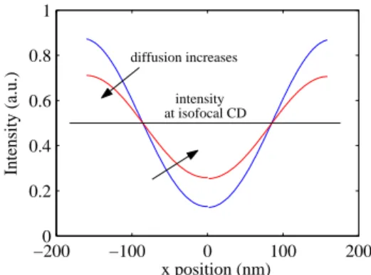
In the previous superposition of experimental & simulated FEM, we have observed (cf. figure 10) that the experimental ones appear like an expansion of the simulated ones around the isofocal CD. It appears that the convolution of the aerial image with a gaussian presents the suitable properties to correct for that. Indeed, as shown in figure 11, the Bossung curves are just expanded around the isofocal CD that itself does not change as illustrated in figure 12. Consequently, the lack of “diffusion” into the “aerial image plus threshold” model, which appears as a source of inaccuracy for CD prediction, can be modeled by a convolution of the aerial image with a given gaussian noise σnoise.

If we report the experimental CD as a function of threshold at best defocus on the simulated one with several gaussian noises, it appears that the best agreement is when σnoise is between 45 and 60 nm for all experimental conditions. An

figure 14 also exhibits a good fit between experimental & simulated E-D diagram for the same gaussian noise values. The CD offset and the gaussian noise of the present model are optimized for all the experiments at the same time. The optimum values for CD offset and gaussian noise that we have found by optimization are 27nm and 52nm respectively. They are taken the same for all experimental conditions. This offset value, obtained using a global fitting procedure (fit of all experiments at the same time) agrees well with the one deduced in paragraph 3.1.2 from isofocal CDs only. Using the optimized parameters (a, b, CD offset, σnoise) the errors between simulated and experimental FEM datasets are

presented in the table 2. The accuracy of the model is determined by the mean error between simulated and experimental data. First, a mean error close to 5% is found for the whole set, which is good if we consider the contribution of the "noise" of the measured experimental data. The difference between the noisy experimental data and a “perfect” experimental dataset seems to represent a large part of the 5% error. On other hand, we can also note that this error decreases very slightly if we only consider a more limited range of +/-20% around the target CD. This points out the good ability of this model to predict CD in a wide exposure and defocus range.

3.3 "Aerial image + variable gaussian convolution through pitch" model

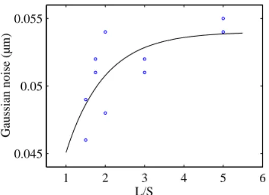
Here, as mentioned in previous works [11], the model presented in this section represents an improvement of the previous one, potentially able to account for resist related proximity bias. It uses a variable gaussian noise, which is an empirical translation of a acid diffusion length varying with the feature pitch. The "aerial image + variable gaussian convolution through pitch" model differs from the previous model only by using increasing gaussian noise for increasing pitch. It models uses two additional parameters. They are obtained by an exponential fit of the best gaussian noises for various pitches found from the previous model. Figure 15 illustrates the variation of the “best gaussian noise” with feature pitch. The best gaussian noise is the one that gives the lowest mean CD error between experiment and simulation if only one feature pitch is used for the fit.

The mean error results between experimental and simulated FEM dataset, which are given in Table 2, are very close to the one of the fixed gaussian noise model. This model seems to offer only a weak improvement of the previous one. Another drawback is that it appears to be hardly predictive because its needs more experiments to define accurately the law of gaussian noise variation through pitch.

Finally, the “aerial image + fixed gaussian convolution” model seems to be sufficient for CD prediction. This can be particular to our experimental dataset, which contains lines not denser than the 1.5 L/S ratio. In this case, the range of gaussian noise is not very large. After figure 18, we can see that it can be much larger if denser features are used. The model described in this paragraph could be of higher interest if we would explore denser line patterns.

3.4 Prediction capabilities of the "aerial image + fixed gaussian convolution" model

In this section we will try to verify that the model detailed in section 3.1.2 is predictive. That means that the model must be able to give accurate results if it is used to simulate CDs for feature type or optical settings outside the set that has been used to fit the model parameters. We use the following procedure:

We fit the model parameters (a, b, CD offset and σnoise) from only four experimental conditions among the ten available

to us. These parameters are used to simulate the CDs for the six remaining experiments. These six remaining datasets are then compared to the experimental ones and should provide good agreement.

As an example, we chose L/S=1.75 and isolated lines to predict experimental FEM for L/S=1.5, 2 and 3. The errors between simulated and experimental FEM datasets are presented in the table 2. The found optimum values, which are CD offset = 26 nm and 51nm gaussian noise, are close to the values which have been found in section 3.2 for the same experimental conditions using the whole set of available data for the fit. Other starting conditions, such as L/S=1.5 and L/S=3 for example, end about to the same results. The mean error is found to be close to the 5% obtained if the whole dataset is used for fitting the model parameters.

4. CONCLUSION

At first, a procedure of fitting the experimental as well as the simulated data has been proposed. We have shown that an expression taking into account simple physical considerations was much more reliable to fit the data (expressed under the form of exposure-defocus matrices) than a very general fitting expression including numerous adjustable parameters. Based on this first phase, the simplest resist threshold model was shown to be not sufficient to give a good match between simulated and experimental data.

Then it has been shown than a simple convolution of the aerial image with a gaussian function can overcome most of the limitations of the simple threshold model by adding only one more adjustable parameter. This gaussian can be viewed as the representation of the photoactive compounds diffusion occurring during the Post Exposure Bake. Indeed, optimum values of 50 to 60nm of gaussian noise, that we have deduced, are in good agreement with published measured diffusion lengths.

After a proper setting of the model parameters to the experimental dataset, discrepancies between simulation and experiment reach 7% in the worst case but can be as small as 2% for certain feature types. Moreover, we have demonstrated that simple gaussian noise convolution models can be predictive. This means that experimental data outside those that have been used to train the model can be simulated with very reasonable accuracy. Significant improvements have been made in resists modeling over the last several years, but simplified resist models such as "aerial image plus gaussian noise convolution" seems to be sufficient for CD prediction, which remain the major demand of IC manufacturers.

ACKNOWLEDGMENTS

This work has been carried out within the European project (MEDEA+ Fluor and IST UV2litho) for 157nm lithography. The authors would like to acknowledge S. Manakli for providing FEM data.

REFERENCES

1. D. Kang, E. K. Pavelchek & C. Swible-Keane, "The accuracy of current model descriptions of a DUV photoresist", Proc. SPIE Vol. 3678, pp. 877-890 (1999)

2. A. Erdmann, W. Henke, S. Robertson, E. Richter, B. Tollkühn, W. Hoppe, "Comparison of simulation approaches for Chemically Amplified Resists", Proc. SPIE Vol. 4404, pp. 99-110 (2001)

3. G. Arthur, B. Martin, C. A. Mack, "Enhancing the development rate model for optimum simulation capability in the sub-half-micron regime", Proc. SPIE Vol. 3049, p. 189 (1997)

4. S. Jug, R. Huang, J. Byers, C. Mack, "Automatic calibration of lithography simulation parameters", Proc. SPIE 4404, p. 380 (2001)

5. A. Sekiguchi, C. A. Mack, M. Isono, T. Matsuzawa, "Measurement of parameters for simulation of Deep UV Lithography using a FT-IR baking system", Proc. SPIE Vol. 3678, pp. 985-1000 (1999)

6. SOLID-C, SIGMA-C GmbH, Thomas-Dehler-Str. 9, 81737 München, GERMANY

7. C. R. Parker, M. T. Reuilly, "Impact of isofocal bias on MEEF management", Proc. SPIE Vol. 4690 (2002) 8. C. Mack, J. Byers, R. Huang, S. Jug, "Automatic calibration of lithography simulation parameters using multiple

data sets", MNE 2001

9. T. A. Brunner and R. A. Ferguson, "Approximate models for resist process effects", Proc. SPIE 2726, pp. 198-207 (1996)

10. J-Y. Yoo, Y-K. Kwon, J-T. Park, D-S. Sohn, S-G. Kim, Y-Su Sohn,"CD Prediction by Threshold Energy Resist Model (TERM)", Proc. SPIE Vol. 4690 (2002)

11. T.H. Fedynyshyn, C.R. Szamanda, and G.J. Cerniglario, "Optimizing the resist to the aerial image in a chemically amplified system", J. Vac. Sci. Technol. B 15 (1997) 2587.

KEYWORDS

Exposure ASML /900 193 nm exposure tool Numerical Aperture 0.63

Partial coherence σ 0.6 and 0.85

Mask Binary mask

Features 120 nm lines

Line to Space ratio L/S 1:1.5, 1:1.75, 1:2, 1: 3 and isolated Resist Sumitomo PAR 700 (0.5µm thick)

CD measurement Hitachi Critical Dimension Scanning Electron Microscope Final CD output metrology precision 3 nm 3σ

Height of measurement 80% from top

Table 1: Experimental conditions

Optical settings Aerial image only model Aerial image + gaussian noise model

Aerial image only + variable gaussian noise model σ S/L Error (whole set) Error (±20% target) Error (whole set) Error (±20% target) Error (whole set) Error (±20% target) 0.6 1.5 14.3 % 12.4 % 4.70 % 2.95 % 4.21 % 2.72 % 0.6 1.75 7.9 % 6.9 % 2.90 % 2.75 % 3.09 % 2.90 % 0.6 2 9.3 % 7.6 % 7.29 % 6.77 % 7.29 % 6.77 % 0.6 3 11.6 % 9.8 % 9.95 % 9.58 % 8.75 % 8.52 % 0.6 Iso 11.8 % 11.4 % 7.34 % 7.73 % 5.72 % 6.05 % 0.85 1.5 16.7 % 13.5 % 3.98 % 4.17 % 4.05 % 3.92 % 0.85 1.75 7.8 % 6.5 % 2.65 % 2.48 % 2.78 % 2.48 % 0.85 2 6.8 % 5.8 % 4.42 % 3.30 % 4.42 % 3.30 % 0.85 3 7.2 % 5.2 % 3.69 % 3.64 % 3.72 % 3.61 % 0.85 Iso 6.7 % 3.8 % 3.77 % 3.67 % 5.43 % 5.02 % Mean error 10.0 % 8.3 % 5.07 % 4.70 % 4.84 % 4.53 %

Table 2: Mean error between simulated and experimental data

−0.40 −0.2 0 0.2 0.4

0.1 0.2

defocus (µm)

CD (µm)

−0.4 −0.2 0 0.2 0.4 0.27 0.28 0.29 0.3 0.31 CD (µm) defocus (µm) 0 0.2 0.4 0.6 0.8 1 0 0.1 0.2 0.3 0.4 threshold CD (µm) isofocal CD threshold at isofocal CD

Figure 2: CD as a function of focus (given threshold) Figure 3: CD as a function of threshold (given focus)

−0.2 0 0.2 0 0.05 0.1 0.15 0.2 0.25 0.3 defocus (µm) CD (µm) −0.40 −0.2 0 0.2 0.4 0.1 0.2 0.3 0.4 defocus (µm) CD (µm)

Figure 4: Fit using equation 1 (solid lines) of simulated FEM data (dotted lines with diamonds)

(120nm lines; σ = 0.85; L/S = 1.5)

Figure 5: Fit using equation 1 (solid lines) of simulated FEM data (dotted lines with diamonds)

(120nm lines; σ = 0.85; L/S = 1.5) −0.40 −0.2 0 0.2 0.4 0.1 0.2 0.3 0.4 defocus (µm) CD (µm) −0.40 −0.2 0 0.2 0.4 0.1 0.2 0.3 0.4 defocus (µm) CD ( µ m)

Figure 6: Final fit using equation 2 (solid lines) of simulated FEM data (dotted lines with diamonds)

(120 nm lines; σ = 0.85; L/S ratio= 1.5)

Figure 7: Final fit using equation 2 (solid lines) of simulated FEM data (dotted lines with diamonds)

−0.4 −0.2 0 0.2 0.4 0.08 0.1 0.12 0.14 0.16 defocus (µm) CD (µm) −0.4 −0.2 0 0.2 0.4 0.08 0.1 0.12 0.14 0.16 defocus (µm) CD (µm) (a) (b)

Figure 8: Final fit using equation 2 (solid lines) of experimental FEM data (dotted lines with diamonds)

for 120 nm lines using σ = 0.6 and: a) L/S ratio= 1.75, b) isolated lines

0.4 0.5 0.6 0.7 0.8 6 8 10 12 14 0.6 ; 1.50 0.6 ; 1.75 0.6 ; 2.00 0.6 ; 3.00 0.6 ; .ISO 0.85 ; 1.50 0.85 ; 1.75 0.85 ; 2.00 0.85 ; 3.00 0.85 ; .ISO threshold at isofocal CD dose at isofocal CD (mJ.cm −2 )

Figure 9: Experimental exposure dose at isofocal CD vs. simulated intensity threshold at isofocal CD, for all experimental conditions

−0.4 −0.2 0 0.2 0.4 0.1 0.15 0.2 defocus (µm) CD ( µ m) −0.4 −0.2 0 0.2 0.4 0.1 0.15 0.2 defocus (µm) CD ( µ m) (a) (b)

Figure 10: Superposition of simulated FEM using the “aerial image plus threshold” model (solid lines) and

corresponding experimental data (dotted lines with diamonds), for 120 nm lines using σ = 0.6 and:

a) L/S = 1.75, b) isolated lines. This superposition based on isofocal CD coincidence, all the thresholds of simulated isothresholds (with increasing isodose CD) correspond to the doses of experimental isodoses using the relation (3)

−0.5 0 0.5 0.08 0.1 0.12 0.14 0.16 0.18 Gaussian noise = 0nm CD ( µ m) −0.5 0 0.5 0.08 0.1 0.12 0.14 0.16 0.18 Gaussian noise = 10nm −0.5 0 0.5 0.08 0.1 0.12 0.14 0.16 0.18 Gaussian noise = 20nm −0.5 0 0.5 0.08 0.1 0.12 0.14 0.16 0.18 Gaussian noise = 30nm −0.5 0 0.5 0.08 0.1 0.12 0.14 0.16 0.18 Gaussian noise = 40nm defocus (µm) CD ( µ m) −0.5 0 0.5 0.08 0.1 0.12 0.14 0.16 0.18 Gaussian noise = 50nm defocus (µm) −0.5 0 0.5 0.08 0.1 0.12 0.14 0.16 0.18 Gaussian noise = 60nm defocus (µm) −0.5 0 0.5 0.08 0.1 0.12 0.14 0.16 0.18 Gaussian noise = 70nm defocus (µm) (a) −0.5 0 0.5 0.08 0.1 0.12 0.14 0.16 0.18 Gaussian noise = 0nm CD ( µ m) −0.5 0 0.5 0.08 0.1 0.12 0.14 0.16 0.18 Gaussian noise = 10nm −0.5 0 0.5 0.08 0.1 0.12 0.14 0.16 0.18 Gaussian noise = 20nm −0.5 0 0.5 0.08 0.1 0.12 0.14 0.16 0.18 Gaussian noise = 30nm −0.5 0 0.5 0.08 0.1 0.12 0.14 0.16 0.18 Gaussian noise = 40nm defocus (µm) CD ( µ m) −0.5 0 0.5 0.08 0.1 0.12 0.14 0.16 0.18 Gaussian noise = 50nm defocus (µm) −0.5 0 0.5 0.08 0.1 0.12 0.14 0.16 0.18 Gaussian noise = 60nm defocus (µm) −0.5 0 0.5 0.08 0.1 0.12 0.14 0.16 0.18 Gaussian noise = 70nm defocus (µm) (b)

Figure 11: Superposition of simulated FEM using the aerial image convolved with an increasing gaussian noise (solid

lines), and corresponding experimental data (dotted lines with diamonds), for 120 nm lines using σ = 0.6 and:

−2000 −100 0 100 200 0.2 0.4 0.6 0.8 1 x position (nm) Intensity (a.u.) diffusion increases intensity at isofocal CD 0.35 0.4 0.45 0.5 0.55 0.05 0.1 0.15 0.2 threshold (A.U.) CD ( µ

m) Gaus.Noise = 70 nmGaus.Noise = 60 nmGaus.Noise = 50 nm

Gaus.Noise = 50 nm

Gaus.Noise = 70 nm diffusion increases

diffusion increases

Figure 12: Aerial image for several gaussian noises Figure 13: Line width as a function of intensity threshold for simulated aerial image convolved

with various gaussian noises

10 12 14 −0.4 −0.2 0 0.2 0.4 Gaussian noise = 0 nm. defocus ( µ m) 10 12 14 −0.4 −0.2 0 0.2 0.4 Gaussian noise = 10 nm. 10 12 14 −0.4 −0.2 0 0.2 0.4 Gaussian noise = 20 nm. 10 12 14 −0.4 −0.2 0 0.2 0.4 Gaussian noise = 30 nm. 10 12 14 −0.4 −0.2 0 0.2 0.4 Gaussian noise = 40 nm. defocus ( µ m) dose (mJ.cm−2) 10 12 14 −0.4 −0.2 0 0.2 0.4 Gaussian noise = 50 nm. dose (mJ.cm−2) 10 12 14 −0.4 −0.2 0 0.2 0.4 Gaussian noise = 60 nm. dose (mJ.cm−2) 10 12 14 −0.4 −0.2 0 0.2 0.4 Gaussian noise = 70 nm. dose (mJ.cm−2)

Figure 14: Superposition of ED diagrams of simulated FEM fits using the aerial image convolved with an increasing gaussian noise (solid lines), and corresponding experimental ones (dotted lines)

1 2 3 4 5 6 0.045 0.05 0.055 L/S Gaussian noise (µm)