HAL Id: hal-01074548
https://hal.archives-ouvertes.fr/hal-01074548
Submitted on 3 Dec 2014
HAL is a multi-disciplinary open access archive for the deposit and dissemination of sci-entific research documents, whether they are pub-lished or not. The documents may come from
L’archive ouverte pluridisciplinaire HAL, est destinée au dépôt et à la diffusion de documents scientifiques de niveau recherche, publiés ou non, émanant des établissements d’enseignement et de
simulations
Mikhael Tannous, Patrice Cartraud, Mohamed Torkhani, David Dureisseix
To cite this version:
Mikhael Tannous, Patrice Cartraud, Mohamed Torkhani, David Dureisseix. Assessment of 3D mod-elling for rotor-stator contact simulations. 11th World Congress on Computational Mechanics (WCCM XI), 5th European Conference on Computational Mechanics (ECCM V), 6th European Conference on Computational Fluid Dynamics (ECFD VI), Jul 2014, Barcelona, Spain. pp.1938-1949. �hal-01074548�
11th World Congress on Computational Mechanics (WCCM XI) 5th European Conference on Computational Mechanics (ECCM V) 6th European Conference on Computational Fluid Dynamics (ECFD VI) E. O˜nate, J. Oliver and A. Huerta (Eds)
ASSESSMENT OF 3D MODELING FOR ROTOR-STATOR
CONTACT SIMULATIONS
MIKHAEL TANNOUS∗, PATRICE CARTRAUD∗, MOHAMED
TORKHANI† AND DAVID DUREISSEIX‡ ∗ G´eM, Ecole Centrale de Nantes, Nantes, France
e-mail: {mikhael.tannous, patrice.cartraud}@ec-nantes.fr
†LaMSID UMR EDF-CNRS-CEA 2832, EDF R&D, F-92141, Clamart Cedex, France
e-mail: [email protected]
‡Universit´e de Lyon, LaMCos, INSA de Lyon, CNRS UMR 5259, Lyon, France
e-mail: [email protected]
Key words: Rotor-stator contact, 3D modeling, penalty, rotor dynamics, finite elements. Abstract. Rotor dynamic problems with rotor to stator contact interactions are most of the time dealt with in the literature by 1D local models. This leads to an affordable simulation time, but the corresponding approximations are difficult to assess. This re-search work highlights the necessity of a 3D model for a more accurate simulation of a rotor-stator contact problem, even if the differences between the 1D and the 3D results are not obvious on the rotor orbits. However, the limitations of the 1D simulations are shown. Indeed, the rigid body section assumption in a beam model of the rotor leads to approximations in the spatial distribution of the contact forces and their intensity. Therefore, the friction torque generated by the contact is overestimated in a 1D model.
1 INTRODUCTION
A turbine accident occurs when a terminal blade is lost, thus generating an important unbalance. So the turbine is decoupled from the generator and slows down under aero-dynamic friction. The turbine vibrations are increased when passing through its critical speed, and rotor to stator contact is observed.
The rotor-stator contact problem is a complex and highly non linear problem, pre-senting both multi-physical (vibrations, contact, thermo-mechanical effects, etc.) and multi-scale (local deformations, etc.) phenomena that are difficult to model and to take into account accurately. The first models proposed in the literature to deal with rotor-stator contact problems are based on a simple Jeffcott rotor (cf. [2] and [3]). Moreover, the rotational velocity is supposed to be constant, and is kept so along the rotor-stator
contact phase by a compensating torque. These simplified models are described by dif-ferential equations and solved analytically, neglecting gyroscopic effects [4, 5].
These approaches remain far from modeling the industrial rotor-stator contact lems. Finite elements approaches can provide a better description of the industrial prob-lems. The rotor and the stator are no more considered rigid as rigid bodies. However, most of the research work in the literature are based on beam models. Recently, a beam model of both the rotor and the stator was used in [8] to simulate the behavior of an industrial EDF turbine during its rotor-stator contact phase, solved via the harmonic balance method. As far as we know, this research as well as that of [1] remain one of the most advanced finite element approaches to describe rotor-stator contact problems. In [1], the slowing down of the turbine due to rotor-stator contact is addressed. However, the rigid body cross-section assumption in beam models are difficult to assess especially in the context of the rotor to stator contact modeling using a beam to beam contact.
This paper aims at illustrating the contribution of a 3D finite elements modeling of the rotor-stator contact interactions. This is achieved by comparing the results of a 3D finite elements model of a rotor-stator contact problem with those obtained by a simplified 1D model. All of the example cases are inspired from true industrial problems of EDF turbines belonging to a Turbo-Alternator Group under operation at EDF nuclear parks. Note that for confidential reasons, some dimensions are hidden or modified.
Code Aster, which is an open source finite element software developed by the Research and Development department at EDF [9], is used for simulating both the 1D and the 3D contact problems. It integrates modern, efficient and easy to use 1D rotor-stator contact capabilities. It is also an open software, more adapted to research problems than commercial softwares.
In the following we present the rotor-stator system under study as well as the optimal choices that have been retained for the 1D and the 3D contact models on Code Aster. The results of these models are compared in section 5, and suitable conclusions are deduced. 2 THE ROTOR-STATOR SYSTEM UNDER STUDY
The study case shown in this article is inspired from the dimensions of a real EDF turbine belonging to a Turbo-Alternator Group (TAG) of a nuclear park. The unbalance is caused by the loss of a terminal blade that generates a local force making the rotor vibrate. In the following models, the unbalance is taken into account by a local force.
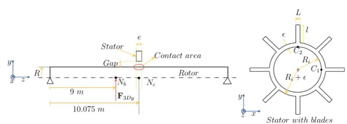
Figure 1 shows the dimensions of the rotor and the stator used in our study cases. To save computational cost, the 3D disk is not modeled, i.e., the rotor consists of a rotating shaft. The left hand side of fig. 1 shows the upper half of the rotor’s cross section. The rotor is 20.15 m long and has a radius R = 1.075 m.
The stator consists of two rings linked by a number of blades. In order to simplify the model, and as done in the thesis of [1], the exterior ring is not modeled and the extremities of the blades are fixed as presented in fig. 1.
Stator
Stator with blades Ri Ri+ ǫ Contact area ǫ Rotor F3Dy Nc Nb 9 m 10.075 m C1 C2 z z y y x x R Gap e L l
Figure 1: Dimensions of the rotor-stator system under study
(along the z axis of fig. 1) is e = 0.15 m. The blades length along the z-axis is equal to that of the ring. The blades are l = 0.755 m long and L = 0.038 m large. The stator mean-line is located on its rotation axis (coincident with point Nc of the rotor). The rotor
is simply supported and subjected at point Nb to an unbalance equivalent to the loss of a
mass of 100 kg at a distance of 2.75 m from the rotation axis spinning at 1500 rpm (this generates a 6.8 × 10⁶ N unbalance force that rotates with the rotor). The component of
this force along the y-direction is presented on fig. 1.
The rotor and the stator are made from steel material having a Young Modulus E = 2.1 × 10¹¹ P a, a density ρ = 7800 kg/m3 and a Poisson coefficient ν = 0.3. Coulomb
friction with µ = 0.02 is considered between the rotor and the stator.
The rotor starts rotating at t = 0 with a null acceleration and reaches its stable and constant rotational velocity ω = 240 rpm at t = 0.01 s, with a null acceleration as described by eq. 1 in section 3.3.
3 ROTOR-STATOR CONTACT MODELING ON CODE ASTER
To the best of our knowledge, 3D rotor-stator contact models are absent from the literature. Reducing the computational cost of 3D rotor-stator contact problems, by coupling 1D and 3D models, was the main concern in [6, 7]. However, no 3D contact modeling was performed.
This research paper presents a first 3D rotor-stator contact modeling on Code Aster, whose capabilities have been updated to the needs of a complex 3D rotor-stator contact modeling.
The 3D contact model constructed, thereby, is consistent with the 1D contact model. 3.1 1D modeling of rotor-stator contact: the choc law
A simple and efficient 1D modeling approach called the choc law [10], and based on a node-to-node contact formulation is available on Code Aster. Its precision and efficiency make it one of the best 1D contact modeling techniques. Gyroscopic effects are taken into account. Recently, the choc law was updated, following the research work of [8], and
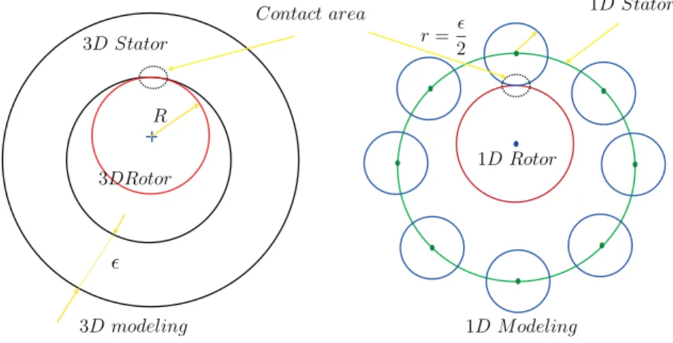
integrates the computations of the rotor-stator friction torque. 3D Stator 1D Stator 3DRotor R Contact area ǫ 3D modeling r = ǫ 2 1D Rotor 1D Modeling
Figure 2: The choc law basics
Figure 2 illustrates the choc law basics. Let us consider a simple stator case, that of a ring having an inner radius R, possessing no blades and of a thickness ǫ. The beam model of such a stator is a set of curved beams forming a circle of radius R + ǫ
2. The Different nodes of the stator are represented by green dots on fig. 2. The rotor’s cross-section in the beam model is presented by a node. This latter is likely to come into contact with the different nodes of the stator. The higher the number of nodes on the stator, the more precise the model. However, the computational cost increases exponentially with the node number. Each node of the stator and of the rotor is assigned to a hard disk that allows to take the nodes distances correctly.
The beam elements of the rotor and of the stator are deformable, thus allowing the different disks to adjust their positions with respect to the rotor and the stator deforma-tions. However, this by-circle hypothesis does not consider the cross-section deformations of the rotor and the stator.
An explicit Runge-Kutta integration scheme represents the optimal choice in Code Aster for 1D rotor-stator contact problems.
3.2 3D modeling of the rotor-stator contact problem on Code Aster
A master-slave contact formulation and a penalty resolution method are the optimal choices for the rotor-stator contact on Code Aster.
The only time integration technique offered by Code Aster for 3D contact problems is a damped Newmark integration technique.
3.3 Limitations of Code Aster
One current limitation of Code Aster is its computational cost for 3D contact modeling due to the implicit integration techniques strictly offered by Code Aster for 3D contact
problems.
Moreover, the rotational velocity is a data of the dynamic problem. Its evolution law is not an unknown of the mechanical problem. Therefore, rotor-stator contact will not lead to a deceleration of the rotor, but rather, will result in stator local deformations, rotor torsions, etc.
In a 1D contact problem, the rotational velocity is given by the user. However, in a 3D contact problem, the rotational velocity is taken into account by imposing the displacements of the rotor’s boundary sections in such a way that the rotor starts from a null acceleration at t = 0 and reaches its constant and given velocity ω at time tm with a
null acceleration: ω(t) = ω × (3 − 2× t tm )t 2 t2 m (1) The contact area is sufficiently far from the boundary sections where the nodal displace-ments are prescribed.
4 CONSISTENCY OF THE 1D AND THE 3D MODELS
The 1D and the 3D models should be consistent so that the only differences between the 1D and the 3D contact models result from the contact methods and algorithms and not from the models themselves.
The rotor of this study case, shown in fig. 1, has a sufficient slenderness and can be modeled by beam elements. The beam and the 3D rotor finite element models exhibit similar behavior and very close natural frequencies. However, the industrial stators are not slender enough to be modeled by beam elements, thus the 1D contact model will consist of a rotor modeled by beam elements, while the stator is a 3D model. The contact between the 1D rotor and the 3D stator is solved via the choc law (section 3.1). The 3D contact model is made with the 3D rotor and the 3D stator.
For further details, please refer to the PhD thesis of Tannous [11]. 5 APPLICATION EXAMPLE
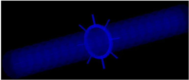
Figure 4 shows simultaneously the 1D and the 3D rotors, as well as the 3D stator that is used in both 1D and 3D rotor-stator contact simulations.
In this study case the stator is meshed quadratically and counts 2280 nodes as shown in fig. 3. 128 nodes belong to the contact surface. Each blade end is fixed, and the stator displacements are blocked along the z-axis (in the direction parallel to the rotor axis).
A damped Newmark integration scheme is used with a time step of 5 × 10⁻⁵ s. For a
one second simulation period, the computational time is 60 hours on a 8 GHz RAM and a Quad2-Core 2.75 GHz CPU computer.
Since the penalty contact method is chosen, a parametric study is lead on the normal and tangential penalty coefficients to ensure that penetrations are negligible and results
Figure 3: 3D model of the rotor-stator system
Figure 4: 1D and 3D models of the rotor-stator system
are not dependent on these coefficients. The nominal values kn = 1014 N/m (normal
contact) and kt = 1010 N/m (tangential contact) are thus taken, since it appears that
multiplying or dividing these coefficients by ten do not lead to solution changes.
Now the results of the 1D and 3D contact models are compared. First, fig. 5 shows a comparison between the orbits of point Nc.
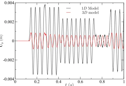
Then, the stator behavior is examined. Figure 6 shows a comparison between the displacements of point C1 (see fig. 1) for a beam and a 3D modeling of the rotor-stator
contact.
It is obvious that the stator, in the beam modeling, has larger displacements (up to three times greater) along the y-axis direction, i.e., along the tangential direction corresponding to the friction force, than the stator belonging to the 3D modeling. This is also true if we check the tangential displacements of point C2 (the x-axis direction) as
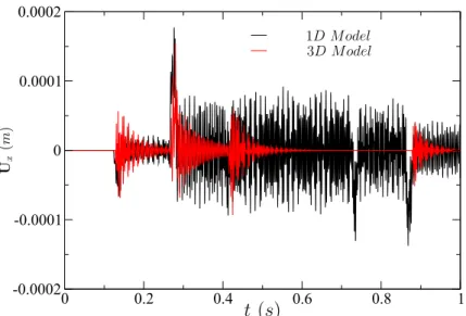
shown on fig. 7. Only the displacements amplitude is different on these points from one model to another. The oscillations frequencies are practically the same. However, these differences are less important in the normal contact direction as shown in fig. 8, which represents the displacements of point C1 along the x-axis direction.
Thus, it is the contact force, both its normal and tangential components, but mainly the tangential one, and therefore the rotor-stator friction torque that differ between the beam and the 3D contact modelings. This is mainly due to the rotor’s cross-section rigidity. In fact, a rigid rotor’s cross-section means a wider contact surface between the
0 0 0.010 0.010 0.005 0.005 −0.005 −0.005 −0.010 −0.010 Uy (m ) Ux(m) 3D rotor model Beam rotor model
Figure 5: Orbits of the 3D rotor and the beam rotor
0 0.2 0.4 0.6 0.8 1 -0.004 -0.002 0 0.002 0.004 1D Model 3D model t (s) Uy (m )
0 0.2 0.4 0.6 0.8 1 -0.004 -0.002 0 0.002 0.004 1D Model 3D Model t (s) Ux (m )
Figure 7: Displacements according to the x-axis of C2
0 0.2 0.4 0.6 0.8 1 -0.0002 -0.0001 0 0.0001 0.0002 t (s) Ux (m ) 1D Model 3D Model
rotor and the stator of the beam model than that of the 3D model. This is obvious in fig. 9 that shows the deformed stators, amplified by a factor of 100, at t = 0.876 s. The stator exhibits a rotation, around its main rotational axis, significantly more important in 1D contact modeling than in 3D. In fact, as fig. 9 shows, the rotation of the stator around its main axis causes blade deflections that are obviously seen on the 1D contact model, while they are negligible on the 3D contact model.
1D Model 3D Model
Figure 9: Comparison of the deformation of 1D and 3D stator models, amplified by a factor of 100
In our study case, and since the rotational velocity of the rotor is a data of the dynamic problem, then the rotor-stator contact will not lead to a rotor deceleration, and leads to a rotation of the stator around its main rotational axis. If the rotational velocity of the rotor is not a data of the dynamic problem, than the rotor-stator contact would have lead to a higher deceleration of the rotor of the 1D contact model than that of the 3D one. This highlights the necessity of a 3D model for the simulation of an accidental slowing down of a turbine. ω u1 u2 u3 u4 u5 u6 u 7 u8
Figure 10: Rotating disk
the 1D contact model and the 3D one. We check in the following the behavior of the stator by decoupling the rotational component from the translational components. This procedure will help evaluate the behavior differences of the 1D and the 3D stators ex-cluding the rotations of the stator induced by the friction torque. For that purpose, eight points belonging to the stator contact surface are chosen so that they are on the same cross-section position as Nc and symmetrically distributed, with respect to the stator
center, every 45 as illustrated in fig. 10.
If ui denotes the displacement vector of point i, then
i=1→8(ui) = 0 is the overall
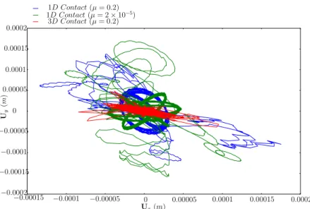
translation of the stator. This sum is called the stator center orbit, and evaluates the displacements of the stator center due to the normal contact. By comparing the stator orbits of the 1D and 3D contact, one can judge the behavior differences of the 1D and 3D stators due to the normal contact, and see if these difference are as significant as the tangential ones. 0 0 0.00005 0.00005 0.0001 0.0001 0.00015 0.00015 0.0002 0.0002 −0.00005 −0.00005 −0.0001 −0.0001 −0.00015 −0.00015 −0.0002 Uy (m ) Ux(m) 3D Contact (µ = 0.2) 1D Contact (µ = 0.2) 1D Contact (µ = 2 × 10⁻⁵)
Figure 11: Stator center orbits comparison
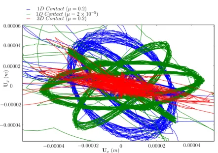
Figure 11 shows the stator center orbits of the 1D and 3D models. On this same figure, we also show stator center orbits of the 1D model with a negligible friction coefficient (µ = 2 × 10⁻⁵). For a better clarity a zoom on fig. 11 is presented in fig. 12. It is obvious
that the stator center orbits of the 1D and the 3D models are very different. Reducing significantly the friction coefficient on the 1D contact model leads to obvious differences, as seen on fig. 11 and fig. 12. However, these difference are less obvious that those found by comparing the 1D and the 3D contact models of the same physical problem (with identical friction coefficients). We therefore conclude that it is not only the tangential behavior of the stator due to the friction torque that is different between the 1D and the 3D models. It is both the normal and the tangential behaviors that are different.
0 0 0.00002 0.00002 0.00004 0.00004 0.00006 −0.00002 −0.00002 −0.00004 −0.00004 Uy (m ) Ux(m) 3D Contact (µ = 0.2) 1D Contact (µ = 0.2) 1D Contact (µ = 2 × 10⁻⁵)
Figure 12: Zoom on the orbits of the stator center
6 CONCLUSIONS
The study case example presented in this article highlights the contribution of a 3D model to a rotor-stator contact problem. In fact, the rigid body cross-section assumption in a beam model, as well as the different assumptions in a simplified 1D contact problem have a strong influence on the contact forces, both their distribution and their intensity, leading therefore, to an overestimated friction torque in a 1D contact model, as well as a global contact behavior that is very different from a 3D one.
ACKNOWLEDGMENTS
The authors thank the French National Research Agency (ANR) in the frame of its Technological Research COSINUS program. (IRINA, project ANR 09 COSI 008 01 IRINA).
REFERENCES
[1] Roques, S. Legrand, M. Cartraud, P. and Stoisser, C.and Pierre, C. Modeling of a rotor speed transient response with a radial rubbing. Journal of Sound and Vibration (2009), 329: 527–546.
[2] Childs, D. Turbomachinery rotordynamics: phenomena, modeling, and analysis. New York : Wiley, (1993).
[3] Al Bedoor, B. Transient torsional and lateral vibrations of unbalanced rotors with rotor-to-stator rubbing. Journal of Sound and Vibration (2007), 229: 627–645.
[4] Karpenko, E. Wiercigrocha, M. Pavlovskaiaa, E. and Cartmellb, M. Piecewise ap-proximate analytical solutions for a Jeffcott rotor with a snubber ring. Journal of
Mechanical Sciences (2002), 44: 475–488.
[5] Chu, F. and Zhang, Z. Bifurcation and Chaos in a Rub-Impact JEFFCOTT Rotor System. Journal of Sound and Vibration (1998), 210: 1–18.
[6] Tannous, M. Cartraud, P. Dureisseix, D. and Torkhani, M. A beam to 3d model switch for transient dynamic analysis. In Proceedings of the 6th European Congress
on Computational Methods in Applied Sciences and Engineering, ECCOMAS 2012,
10-14 septembre 2012, Vienna, Austria.
[7] Tannous, M. Cartraud, P. Dureisseix, D. and Torkhani, M. Bascule d’un mod`ele poutre `a un modle 3D en dynamique des machines tournantes. 11`eme Colloque
na-tional en calcul des structures, CSMA 2013, Presqu’ˆıle de Giens, Var, 2013.
[8] Peletan, L. Baguet, S. Torkhani, and M. Jacquet Richardet, G. A comparison of stability compu- tational methods for periodic solution of nonlinear problems with application to rotordynamics. NonLinear Dynamics, Springer (2013).
[9] EDF R&D: Code Aster: A general code for structural dynamics simulation under gnu gpl licence. http://www.code-aster.org, (2001).
[10] Alarcon, A. R5.06.03 Mod´elisation des chocs et du frottement en analyse transitoire par recombinaison modale. Tech. Rep., EDF R&D, (2011).
[11] Tannous, M. D´eveloppement et ´evaluation d’approches de mod´elisation num´erique
coupl´ees 1D et 3D du contact rotor-stator. PhD thesis, Ecole Centrale de Nantes