Numerical strategy for dynamic simulation of impacts on SFR fuel pins and experimental validation

HAL Id: cea-02339668

https://hal-cea.archives-ouvertes.fr/cea-02339668

Submitted on 4 Nov 2019

HAL is a multi-disciplinary open access

archive for the deposit and dissemination of

sci-entific research documents, whether they are

pub-lished or not. The documents may come from

teaching and research institutions in France or

abroad, or from public or private research centers.

L’archive ouverte pluridisciplinaire HAL, est

destinée au dépôt et à la diffusion de documents

scientifiques de niveau recherche, publiés ou non,

émanant des établissements d’enseignement et de

recherche français ou étrangers, des laboratoires

publics ou privés.

on SFR fuel pins and experimental validation

T. Catterou, V. Blanc, G. Ricciardi, S. Bourgeois, B. Cochelin

To cite this version:

T. Catterou, V. Blanc, G. Ricciardi, S. Bourgeois, B. Cochelin. Numerical strategy for dynamic

simulation of impacts on SFR fuel pins and experimental validation. Nuclear Engineering and Design,

Elsevier, 2018, 340, pp.73-85. �10.1016/j.nucengdes.2018.09.021�. �cea-02339668�

T. Catterou

_{, V.Blanc}

_{, G.Ricciardi}

_{, S.Bourgeois}

_{, B.Cochelin}

Abstract. — Fuel pins are the first containment barriers of a sodium fast reactor, and their integrities have to be

preserved during a dynamical load. Pins are included in an assembly with mounting gaps, to allow them to swell during the life cycle of the reactor; so they are subjected to shock and contact at the early ages. A numerical method has been chosen with the aim to determine the dynamical behavior of a large system with a lot of contacts. The validity of the method is confronted for a basic issue to semi-analytical solution. Then, dynamical behavior of an isolated pin has been studied experimentally and numerically, with a non-linear representative contact law. Numerical method is appropriate to assess contact forces caused for pins.

Keywords — Dynamic, modal analysis, contact, finite-element.

Nomenclature

Nomenclature

𝑈: Deflection vector m : Mass of the beam

𝐹𝑠: Impact forces 𝑴, 𝑪, 𝑲 : Mass, damping and stiffness matrices – physical basis

𝐹: External forces 𝑴̅ , 𝑪̅, 𝑲̅ ∶ Mass, damping and stiffness matrices – modal basis 𝛿: Contact deflection 𝜉𝑖 : Structural damping – mode i

𝑑𝑡 : Time step 𝑘𝑠 : Shock stiffness

𝑑𝑡𝑠: Contact time 𝑘𝑏 ∶ Bending stiffness

Φ𝑖: Mode shape – mode i 𝑅𝑘 : Ratio of shock and bending stiffness. (𝑘𝑠/𝑘𝑏)

𝑄𝑖: Modal displacement – mode i 𝑓𝑡𝑟𝑢𝑛𝑐: Frequency truncation of numerical computation

𝜔𝑖: Pulsation – mode i 𝑅𝑓𝑡𝑟𝑢𝑛𝑐: Ratio of 𝑓𝑡𝑟𝑢𝑛𝑐 and first natural mode frequency

E : Young’s Modulus 𝐸𝑟𝑟, 𝐸𝑟𝑟𝐹: Error indicator on PSD and forces

I : Inertia 𝑢0, 𝑢̇0: Initial displacement and velocity

L : Length 𝑑1: Release amplitude

Γ: Power spectral density

I.

Introduction

I.1

Industrial context

In sodium fast reactor (SFR), the fuel is enclosed in pins, composed of slender steel tubes (the clad) and a spacer wire coiled into a helix around the clad (Figure 1-a). The pin has a very heterogeneous distribution of mass since fuel pellets represent 70% of the total mass. Details on design are given by (Beck et al., 2017).

Figure 1 – ASTRID fuel pin (a) and sectional view of the pins bundle in its wrapper tube (b)

Fuel pins are arranged in a bundle enclosed inside a hexagonal tube (Figure 1-b). Many hundreds assemblies are main constituents of the reactor core. These assemblies are maintained by their spikes (Figure 2) at the bottom of the core in a lattice. During a dynamic loading, the core lattice shakes assemblies which will bend and impact each other locally on spacer pads. The shock will generate acceleration on pins and cause dynamic stresses. Then, a high number of pin-to-pin collisions, up to 15000, will occur in the bundle between the spacer wire of a pin and the clad of a nearby one.

Figure 2 - Schematic of two assemblies

The industrial aim is to develop a calculation methodology to identify contact force on pins caused by dynamic loads (earthquake, handling or transportation), throughout the life of the assembly. Then, a local model will allow assessing maximum stresses in pins and sizing them. The accuracy of the calculation methodology has to be approved by analytical and experimental reference. This work differs from the other ones on the dynamic of fuel assemblies (Broc et al., 2014; Moussallam et al., 2011) because the study is focused on the pins bundle without fluid.

I.2

Contact dynamics modelling

Multibody collisions are one of the strongest non-linearity in mechanics. Contact modelling is an ancient topic, which starts with works of (Hertz and al., 1896) on the contact between two optical lenses. Many authors have expanded thereafter this theory by introducing friction, tangential force and dynamic effects (Johnson, 1985; Stronge, 2004). But, the numeric implementation of a contact remains very complex, whereas it is usually met in industrial context. Impacts occur during very brief time, and cause high forces and accelerations (Gilardi and Sharf, 2002). Standard numerical methods struggle to converge or to remain stable, leading to inaccurate or very slow calculation (Bathe, 2006). Several dedicated integration scheme have been created to solve contact problem, using a time-step cutting (Bathe, 2007), energy consistency (Chawla and Laursen, 1998) or high frequency damping (Tchamwa and al., 1999). There are two main kinds of integration scheme, implicit ones for which is an iterative process minimizing the error, and the explicit ones where the calculation is direct. In most cases, explicit schemes are more relevant to deal with contact issue, because they are way faster than implicit ones and remain stable as long as time step is short (less than a millisecond) (Bathe, 2006). But implicit schemes are sometimes used when it is preferable to use a larger time step (Khenous and al., 2006; Thenint, 2011). The integration scheme choice and the manner to model contact are closely linked so they have to be chosen in accordance. Location of contact is usually founded with a dedicated algorithm but it’s not necessary in the bundle because contact zones are known. There are several ways to model the contact in structural dynamic, summarized by (Gilardi and Sharf, 2002). There are two major categories: non-smooth laws, for which the contact is instantaneous and the velocity is discontinuous, versus smooth laws for which solids in contact will be able to interpenetrate each other. In non-smooth dynamics, a restitution parameter is introduced to model the damping (Jean, 1999; Schindler and Acary, 2014; Thornton, 1997), the ratio between absolute values of velocity before and after the shock. In smooth dynamic, a non-linear force is introduced with a penalty method depending on the distance between reference points of solids in contact (Goldsmith, 1960). Several formulations of the contact laws can be found in literature (Gilardi and Sharf, 2002), from the expression of (Hertz et al., 1896) or more complex formulation such as (Thornton, 1997). These laws have been confronted to solve the Newton’s cradle (Donahue and al., 2008). In order to assess contact forces, a smooth law is best suited and can be introduced in a computation with an explicit integration scheme (Gilardi and Sharf, 2002).

Dynamic simulations involving contacts require vast computing power, because of the necessity to use short time-step. There are several ways to simplify the problem, for instance modal analysis which can be used for non-linear calculation (Antunes, 1991) even if it’s not commonly done. If the modal truncation is chosen efficiently (Rieger, 1986), it allows to reduce drastically degrees of freedom of the model and thus lower computation time, allowing the simulation of whole system.

II.

Numerical model and computation methodology

All calculations shown in the follow-up have been made with the finite-element software CAST3M for numerical aspects and Scilab for reference computations. The final goal of the study is to be able to assess the dynamical behavior of the full bundle of 217 pins, with 15000 contact zones and thus it is needed to choose a suitable numerical methodology.

Figure 3 – a) Sub-assembly section. b) Schema of contacts

Contact points are known, they are located between a wire and a clad (Figure 3-a) or a wire and one surface of the wrapper tube (Figure 3-b), depending on the orientation of the wires. Due to the large size of the issue, shell or three dimensional elements are unsuitable. The slenderness ratio between contact points is less than 10, so shear effects are not negligible. Therefore it has been chosen to use Timoshenko beams, with a shear coefficient linked to the pin’s geometry equal to 0,5 (Cowper, 1966).

The objective is to define a numerical method suitable for the whole sub-assembly, but in this paper, only the behavior of a single pin with its contact is studied to assess the validity of the method. Numerical goal is to solve the equation of dynamics with non-linear contact forces, with 𝑴,𝑪 and 𝑲 respectively matrices of mass, damping and stiffness of the pin, 𝐹𝑠 non-linear contact forces and 𝑈 the deflection vector. Contact force at a contact point

𝑓𝑠𝑖 depends on the contact stiffness 𝑘𝑠 and deflection at this point 𝛿𝑖.

𝑴𝑈̈ + 𝑪𝑈̇ + 𝑲𝑈 = 𝐹𝑠(𝑈), (1)

{𝑓𝑠𝑖= 𝑘𝑠𝛿𝑖 𝑖𝑓 𝛿𝑖< 0

𝑓𝑠𝑖= 0 𝑖𝑓 𝛿𝑖> 0 (2)

Usually, mechanical numerical computations are made in the physical basis and with implicit integration scheme, to have a stable and accurate solution. But computation time is heavily linked to the size of the matrices 𝑴, 𝑲 and 𝑪 used. So a modal reduction has been chosen. Eigen modes Φ are obtained by solving the following equation:

This calculation gives the eigenvalues 𝜔_𝑖 and the eigenvectors Φ_i of the structure. To solve the dynamic issue, we use the formula (1) written on the physical basis. The displacement of the structure is being sought in the form (4) using modal analysis, with 𝑄𝑖 modal displacement which depends solely of the time.

𝑈𝑡_{= ∑ Φ} 𝑖𝑄𝑖(𝑡) 𝑁

1

(4)

N is the number of modes considered and is linked with the frequency truncation which will be discussed in section III.4. If N is far below the number of degree of freedom of the mesh, the size of the problem is considerably decreased. The equation (1) can be re-written using the decomposition (4) :

𝑴̅ 𝑄̈ + 𝑪̅𝑄̇ + 𝑲̅𝑄 = 𝜱𝑇_𝐹

𝑠(𝑈) (5)

𝑴̅ , 𝑪̅ and 𝑲̅ are respectively modal mass, damping and stiffness matrices projected on modal basis 𝚽. By construction, matrices 𝑴̅ and 𝑲̅ are diagonals. The damping is defined by damping ratio 𝜉𝑖 related to each mode,

so in this model 𝑪̅ is also diagonal. Therefore, computation will be substantially accelerated.

Contact non-linearities make the implicit scheme convergence very difficult, which lead to unacceptable computation time. Consequently, an explicit integration scheme is chosen, for instance the simplest one, the central difference scheme (Bathe, 2006). By substituting expression of the central difference scheme in the formula (5), it leads to:

( 1 𝑑𝑡2𝑴̅ + 1 2𝑑𝑡𝑪̅) 𝑄𝑡+𝑑𝑡= 𝜱𝑇𝐹𝑠𝑡(𝜱𝑄𝑡) − (𝑲̅ − 2 𝑑𝑡2𝑴̅ ) 𝑄𝑡− ( 1 𝑑𝑡2𝑴̅ − 1 2𝑑𝑡𝑪̅) 𝑄𝑡−𝑑𝑡 (6)

Thus, for every time step, one computation of the modal contribution is simply done (6). Velocities and accelerations are derived from the displacement by using expressions of the integration scheme. This methodology allows really fast computation, but produce instability as soon as the time step is too large in relation to contact time. These aspects will be detailed in section III.5. The contact forces vector is defined on “physical” basis, it depends on the deflection vector 𝑈. So during the computation, physical displacement of each contact point is calculated, contact forces are deducted from these displacements and contact force are projected on the set of modal basis (Boyere, 2010).

The use of an explicit scheme and the reduction of the number of degree of freedom lead to very fast computation. But it is needed to use an analytical reference to choose parameters of the numerical method. Then, an experimental validation is carried out in the last section.

III.

Numerical parameters sensitivity

III.1 Presentation of the issue

A simple contact problem is spotlighted here, a clamped beam in flexion which impacts on a spring at the other edge. This issue is a simplified model of the dynamic behavior of an assembly impacting another one as described in Figure 2 and is similar to the configuration studied by (Yin et al., 2007).The beam is described with its bending rigidity 𝑘𝑏 equal to 3𝐸𝐼/𝐿3, with 𝐸 its Young’s modulus, 𝐼 its inertia and L its length and

represented Figure 4. The problem is solved with the numerical method proposed in section II and compared to a reference semi-analytical method described in Annex A.

Figure 4 - Clamped beam impacting on a spring.

A calculation made with modal analysis requires defining a modal truncation, which means a maximum of natural frequency. The influence of this parameter will be the first step of our comparison. Then time step choice

is very important in an explicit computation. On one hand, a large time step may cause integration scheme instability, on the other hand, a very small time step will increase computation times, storage capacity needed, and doesn’t always lead to more accurate results. Finally, the influence of the spatial discretization, that means the number of elements 𝑛𝑒𝑙𝑒𝑚 used to model the beam, will be analyzed in this section.

III.2 Adimensionnal parameters

The numerical problem of the clamped beam impacting on a spring is solved with the Finite Element software CAST3M. Computations have been made with the explicit integration scheme of central differences and using projection on modal basis described in section II. All the results are observed according to the dimensionless factor 𝑅𝑘, ratio of bending and shock stiffnesses, which represent the ‘hardness’ of the contact (7).

The maximal 𝑅𝑘 value which can be found in the pin’s bundle is about 3000.

𝑅𝑘=

𝑘𝑠

𝑘𝑏=

𝑘𝑠𝐿3

3𝐸𝐼 (7)

The frequency truncation has a significant effect on result and will be observed through another dimensional factor, with 𝑓0 the first eigenmode frequency of the fixed-free beam :

𝑅𝑓𝑡𝑟𝑢𝑛𝑐 =

𝑓𝑡𝑟𝑢𝑛𝑐

𝑓0

𝑓0=1,76_𝜋𝐿2 √𝐸𝐼_𝜌𝑆

(8)

The beam used is representative to the full assembly. Its parameters are 𝑘𝑏 = 4,5.105𝑁/𝑚, total mass 𝑚 =

127𝑘𝑔 and the computation time step is 𝑑𝑡 = 5.10−5_𝑠.

Figure 5 show the displacement of the free-edge of the beam during time obtained by numerical and reference method for two values of 𝑅𝑓𝑡𝑟𝑢𝑛𝑐. Numerical estimation is way better when a high number of modes are

considered, so when 𝑅𝑓𝑡𝑟𝑢𝑛𝑐 is high (Figure 5 – a).

Figure 5 - Displacements on the beam's end for numerical computation and analytical reference for 𝑹𝒌= 𝟑𝟎𝟎𝟎. a) 𝑹𝒇𝒕𝒓𝒖𝒏𝒄= 𝟑𝟎𝟎 b) 𝑹𝒇𝒕𝒓𝒖𝒏𝒄= 𝟏𝟎

The contact force is a very short phenomenon. Figure 6 shows the evolution of the first contact force with the analytical and the numerical computation for two values of 𝑅𝑓𝑡𝑟𝑢𝑛𝑐. A high value of 𝑅𝑓𝑡𝑟𝑢𝑛𝑐 is necessary to

reproduce correctly the contact force. Two contact durations are introduced: 𝑑𝑡𝑠1 the duration of the rebound and

Figure 6 - Forces on the beam's end for numerical computation (green) and analytical reference (black) for 𝑹𝒌= 𝟑𝟎𝟎𝟎. a) 𝑹𝒇𝒕𝒓𝒖𝒏𝒄= 𝟑𝟎𝟎 b) 𝑹𝒇𝒕𝒓𝒖𝒏𝒄= 𝟏𝟎

Some assessment tools are necessary to quantify differences between numerical results and references ones. An error indicator 𝐸𝑟𝑟 (9) is introduced in order to quantify differences between power spectral densities (PSD) Γnum and Γ𝑟𝑒𝑓 obtained with the two methods. This value falls between 0% (superposed signals) and 100%

(decorrelated signals),

𝐸𝑟𝑟 = 𝑚𝑎𝑥(|𝛤𝑛𝑢𝑚− 𝛤𝑟𝑒𝑓|)

𝑚𝑎𝑥([|𝛤𝑛𝑢𝑚|, |𝛤𝑟𝑒𝑓|]) (9)

This function accounts for the correlation between numerical curves and reference ones. For instance, 𝐸𝑟𝑟 = 35% for Figure 5 b).It is globally responsive to amplitude or phase error, but doesn’t take into account short signal variations like contacts.

Thus, another assessment tool based on the ratio of contact forces is used. It compares maximal impact forces recorded during the numerical calculation 𝐹𝑠_𝑛𝑢𝑚 and the reference one 𝐹𝑠_𝑟𝑒𝑓:

𝐸𝑟𝑟𝐹=

𝑚𝑎𝑥 (|𝐹𝑠𝑛𝑢𝑚− 𝐹𝑠𝑟𝑒𝑓|)

𝑚𝑎𝑥 (|𝐹𝑠_𝑛𝑢𝑚|, |𝐹𝑠_𝑟𝑒𝑓|)

(10)

It is defined between 0% (same contact forces) and 100% (contact forces infinitely distinct). The 𝐸𝑟𝑟𝐹 error for

the curves plotted Figure 6 a) is 𝐸𝑟𝑟𝐹= 2% and for Figure 6 b), 𝐸𝑟𝑟𝐹= 50%. These assessment parameters will

be used to observe the influence of modal truncation, time step choice and spatial discrepancy. There is a link between shock duration and minimal value of numerical parameters. The first step of the study is to assess the value of the shock duration.

III.3 Shock duration criterion

The value of the contact stiffness will affect the shock duration. The higher the value of 𝑅𝑘, the faster the shock

will occur and the numerical calculation will require smaller time step and higher frequency truncation. Two different characteristic times are defined. The first one is called 𝑑𝑡𝑠1 and corresponds to the rebound duration,

the period during which bending waves move from contact point and return. For the clamped beam studied here, assumption will be made than only the first clamped-spring mode influence can be taken into consideration to assume this characteristic time. The first pulsation 𝜔𝑠1 of the clamped-spring configuration is computed thanks

to the Rayleigh-Ritz method (Rayleigh, 1896) and is described in Annex B.* 𝑚1 is the total mass of the pin.

*

Note that pulsation modes in the clamped spring configuration can also be determined semi-analytically (Behn et al., 2014) but doesn’t lead to analytic formulation

𝜔𝑠12 =

1512 𝑘𝑏

𝑚1

𝑅𝑘2+ 15 (𝑅𝑘+ 1)

19𝑅𝑘2+ 459𝑅𝑘+ 5436 (11)

The shock duration is equal to:

𝑑𝑡𝑠1=

𝜋

𝜔𝑠1 (12)

The expression (12) gives a good estimate of the rebound duration of the beam. But it doesn’t represent the hardness of the contact, since when 𝑅𝑘 is high, 𝑑𝑡𝑠1 becomes independent of 𝑅𝑘†. A second characteristic time

𝑑𝑡𝑠2 is introduced, depicting the shock duration of a mass impacting on the spring 𝑘𝑠. The mass 𝑚2 considered is

equal to 3/8 of the total mass of the beam, corresponding to the reaction force on the spring for the static problem of a beam submitted to a distributed load.

𝑑𝑡𝑠2= 𝜋√

𝑚2

𝑘𝑠 (13)

The period 𝑑𝑡𝑠2 represents the first vibration period during the contact, whereas 𝑑𝑡𝑠1 represents the full rebound

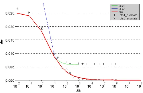
duration as illustrated in Figure 6. So the minimal contact duration 𝑑𝑡𝑠 is the minimum of 𝑑𝑡𝑠1 and 𝑑𝑡𝑠2 and is

plotted Figure 7.

𝑑𝑡𝑠= 𝑚𝑖𝑛(𝑑𝑡𝑠1, 𝑑𝑡𝑠2) (14)

An estimation of 𝑑𝑡_𝑠1 and 𝑑𝑡_𝑠2 is also given thanks to the semi-analytical model (𝑑𝑡_𝑠1_𝑒𝑠𝑡𝑖𝑚𝑎𝑡𝑒 and 𝑑𝑡𝑠2_𝑒𝑠𝑡𝑖𝑚𝑎𝑡𝑒). Formulas (12) and (13) are able to estimate correctly the contact duration of the beam

regardless of the contact stiffness.

Figure 7 – Contact duration depending on Rk

Frequency of the shock is equal to 1/𝑑𝑡𝑠. To model phenomena occurring during the contact duration, frequency

truncation has to be higher (arbitrarily a factor 4 is used) than the frequency of the shock.

𝑓𝑡𝑟𝑢𝑛𝑐> 4 𝑑𝑡𝑠 (15) † _{When 𝑅} 𝑘→ ∞, 𝑑𝑡𝑠1= 𝜋√_1512𝑘19𝑚1 𝑏

Furthermore, explicit scheme have a standard criterion to avoid divergence (Bathe, 2006) : 𝑓𝑡𝑟𝑢𝑛𝑐<

1

4𝑑𝑡 (16)

Time step have to be chosen depending of the frequency truncation if equation (15) and (16) are respected.

𝑑𝑡 <𝑑𝑡𝑠

16 (17)

III.4 Modal truncation influence

Exploit high frequency modes will give a better modeling of contact non-linearities, but will increase calculation cost and cause instabilities. The function 𝐸𝑟𝑟 and 𝐸𝑟𝑟𝐹 are plotted Figure 8, depending on the stiffness ratio and

for various modal truncation ratio. The time step chosen is 𝑑𝑡 = 5.10−5_{𝑠 and 𝑛}

𝑒𝑙𝑒𝑚= 150.

Figure 8 - Error function depending on modal truncation

Vertical dotted lines represent the inequality (15) for each value of 𝑅𝑓𝑡𝑟𝑢𝑛𝑐. For a low modal truncation

(𝑅𝑓𝑡𝑟𝑢𝑛𝑐= 10) and a 𝑅𝑘 higher than 103, 𝐸𝑟𝑟 is about 34% (Figure 8). It represents an overvaluation of the

amplitude of about 30% and a phase offset (Figure 5 - b). With a higher modal truncation, analytical and numerical displacements are more or less the same and the error function is close to zero (Figure 5 - a). Then, when 𝑅𝑘 is very high (>105 here, but the value depends on the time step chosen, see section III.5), computation

diverges because of shocks.

Forces are derived three times from the displacement, so higher differences in results are expected. We compare ratio of force 𝐸𝑟𝑟𝐹 on the Figure 9.

The contact force is overall well computed for low 𝑅_𝑘(<50) but the ratio 𝐸𝑟𝑟_𝐹 increases for higher 𝑅_𝑘 with a small frequency truncation. A 𝑅_{𝑓𝑡𝑟𝑢𝑛𝑐} > 300 is needed to minimize error for 𝑅_𝑘< 3.103 (~20% maximum error). When the frequency truncation used doesn’t respect the equation (15), reference and numerical models begin to diverge. This observation gives a criterion to choose the frequency truncation depending on the contact stiffness.

III.5 Time discretization influence

The aim of this part is to choose the higher time step ensuring unconditional stability of numerical computation. A high frequency truncation, high number of elements and different time steps are used for the simulation (𝑅𝑓_{𝑡𝑟𝑢𝑛𝑐}= 300 𝑎𝑛𝑑 𝑛𝑒𝑙𝑒𝑚= 150). The time step chosen have to respect equation (16). When the time step 𝑑𝑡 is

too high, computation diverges regardless 𝑅𝑘. Note that for a structure with damping, minimal time step can be a

little bit higher (Bathe, 2006). Then, evolution of 𝐸𝑟𝑟 for different values of 𝑅𝑘 is given Figure 10. Criterion (17)

is given with vertical dotted line on the figure.

Figure 10 - Error function depending on temporal discrepancy

For 𝑑𝑡 = 1.10−4_{𝑠, the time step doesn’t comply with criterion (16), so the computation diverges for any 𝑅} 𝑘. For

the other values of 𝑑𝑡, numerical results are similar to reference ones (𝐸𝑟𝑟 < 20%), then diverge for high 𝑅𝑘. A

smaller time step enables good displacement assessment for 𝑅𝑘> 104, even if criterion (15) on the frequency

truncation is not verified. But the contact force is misjudged (Figure 11). The frequency truncation is the main parameter to take into consideration in the methodology of choice (see section III.7).

III.6 Spatial discretization influence

The finite element method requires discretizing the geometry in quite a few elements. In most case, a substantial number of elements increase accuracy but increase also the cost of the computation. Yet, computation showed that force and displacement accuracy is marginally affected to the choice of elements length, as long as the criterion in the literature (Marburg, 2002) is respected (18):

𝑑𝑥 <𝜆 4= 𝑐𝑏𝑒𝑛𝑑𝑖𝑛𝑔 4𝑓𝑡𝑟𝑢𝑛𝑐 𝑐𝑏𝑒𝑛𝑑𝑖𝑛𝑔= √2𝜋𝑓𝑡𝑟𝑢𝑛𝑐√ 𝐸𝐼 𝜌𝑆 (18) Elements have to be small enough to model a bending wave at the frequency 𝑓𝑡𝑟𝑢𝑛𝑐. Otherwise, there is a risk

making mistake if the contact time is very short, so when 𝑅𝑘 is high.

III.7 Numerical parameters choice methodology

For a dynamic simulation with shock based on modal basis, the choice of frequency truncation is of the utmost importance. When the shock stiffness is high confronted to bending stiffness of a structure, it’s needed to increase the frequency truncation or the numerical result will be incorrect. Limit values are given by equations (15) and (16). Once frequency truncation has been chosen, the choice of time step value is self-evident: it has to follow equation (17). To observe very fast phenomena, a lower value of time step is practicable without prejudice to the stability of the computation, but results will not be more accurate. Then, spatial discretization has to be chosen dependently of the truncation frequency but has a minor effect on the stability and the accuracy of the problem. The methodology of choice of numerical parameters for a dynamic simulation with shocks on modal basis has to follow the steps given in Table 1.

This methodology applied to the small fractional horsepower compressor studied by (Yin et al., 2007) gives a frequency truncation value 𝑓𝑡𝑟𝑢𝑛𝑐 > 1,51 𝑀𝐻𝑧. Yet, approximatively above this value of frequency truncation,

results in terms of impact force converged.

Table 1 - Methodology

Step Description Criterion

1 Estimation of shock duration 𝑑𝑡𝑠

2 Choice of the frequency truncation 𝑓_{𝑡𝑟𝑢𝑛𝑐} 𝑓_{𝑡𝑟𝑢𝑛𝑐} > 1/4𝑑𝑡_𝑠 3 Choice of time step 𝑑𝑡 𝑑𝑡 < 1/16𝑑𝑡_𝑠 4 Choice of spatial discretization 𝑑𝑥 𝑑𝑥 < 𝑐_{𝑏𝑒𝑛𝑑𝑖𝑛𝑔}/4𝑓_{𝑡𝑟𝑢𝑛𝑐}

IV.

Experimental validation

IV.1 Description of the test bed

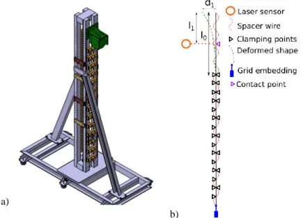
A test bed has been settled in the CEA of Cadarache, to represent the dynamical behavior of a fuel pin in an arrangement similar to the one in the bundle. It is able to load the fuel pin with a shaker and to make free bending release experiment. A CAD model of the device is given Figure 12-a). Two rows of contact elements are set on each side of the fuel pin. Piezoelectric sensors inserted inside contact elements provide dynamical force measurement. Laser sensors provide measurement of the velocity on different points of the pin.

a)

b)

Figure 12 - a) Cad model of the test bed CARNAC, b) Schematic description of the bending tests

Bending release experiments have been made to compare experimental result with the numerical method described above (Figure 12-b)). Several supports have been implemented along the pin except for a free length 𝑙0. The pin is manually bended through a amplitude 𝑑1 at its edge. Velocity and contact force are measured on a

contact point at a height 𝑙1. A rigid stop equipped of a piezoelectric sensor is fixed at the same height for of the

tests. Several parameters have been analyzed:

 The material used for fake fuel pellets, called here 𝑚𝑎𝑡1 and 𝑚𝑎𝑡2. The distribution of mass is

respected with each material.

 The free length: 600, 700 or 800mm with respectively associated mass 316, 376 and 436g.

 The amplitude of release 𝑑1

IV.2 Contact law

Experimental results are compared to the ones given by the numerical method set in section II. Mass, free length, magnitude of release, and geometrical properties of the beam are issued of characteristics of experiment. Linear contact law with stiffness 𝑘𝑠 similar to the section III doesn’t represent well the pin’s geometry. So the contact

law used is non-linear; it takes into account linear ovalization of the wire and the clad and the hertzian deformation on contact areas and (Figure 13).

Figure 13 - Contact model

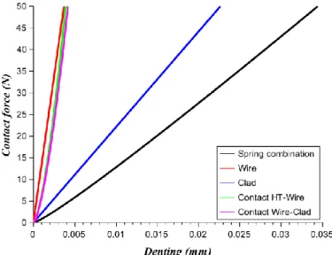
Wire’s and clad’s rigidities 𝑘𝑤𝑖𝑟𝑒 and 𝑘𝑐𝑙𝑎𝑑 are computed analytically by using Fourier series decomposition and

a quasi-punctual force written as a sum of sinus, it’s possible to obtain the ovalization of the tube and cylinder depending on the boundary condition of the problem. The ratio between the force amplitude and the displacement at the load point gives the linear rigidities. Non-linear spring rigidities between the stop and the wire 𝑘̃_ℎ1 and between the wire and the clad 𝑘̃_ℎ2 have been also calculated analytically using Hertz equations (Johnson, 1985). The combination effect of these four springs is calculated using formulas:

𝛿 = 𝐹 ( 1 𝑘𝑤𝑖𝑟𝑒+ 1 𝑘𝑐𝑙𝑎𝑑) + 𝐹 2 3 ( 1 𝑘̃ℎ1 + 1 𝑘̃ℎ2 ) 2 3 𝐹 = − 𝑏 3𝑎+ (− 1 2(𝑞 + √ 4𝑝3_{+ 27𝑞}2 27 )) 1 3 + (−1 2(𝑞 − √ 4𝑝3_{+ 27𝑞}2 27 )) 1 3 with : 𝑎 = 1 𝑘𝑤𝑖𝑟𝑒+ 1 𝑘𝑐𝑙𝑎𝑑; 𝑏 = 1 𝑘̃ ℎ1 + 1 𝑘̃ ℎ2 ; 𝑝 = 𝑏2 3𝑎2; 𝑞 = 2𝑏3 27𝑎3− 𝛿 𝑎 (19)

Numerical values of stiffness are indicated in Table 2.

Table 2 - Stiffness values

𝑘𝑐𝑙𝑎𝑑 𝑘𝑤𝑖𝑟𝑒 𝑘̃ℎ1 𝑘̃ℎ2

2,48.106 _{𝑁/𝑚 1,56.10}7 _{𝑁/𝑚 6,5.10}9 _𝑁/𝑚2_{3 5,85.10}9 _𝑁/𝑚2₃

The whole contact law and the contact law of each of its constituents of the system are plotted Figure 14 :

Figure 14 - Contact law

IV.3 Comparisons between experiments and numerical method

Comparisons have been made on velocity. During an impact, the absolute value of the velocity decreases abruptly, and remains close to zero during the contact time. Then, the pin bounces until another contact time (Figure 15).

Figure 15 - Experimental measurement of velocity, contact time and rebound

An approximation has been made of a unique modal damping for all fixed-free vibration modes of 3%, which corresponds to an average value of the damping generated by dry friction. This choice leads to good result for a short duration study on the first contacts. Initial time set when the velocity is maximal. Experimental simulations have been made for different free length (600, 700 and 800mm), which means for different ratio 𝑅𝑘 (900 −

1430 − 2130). Numerical parameters chosen and the value of criteria of section III.7 are indicated in Table 3. Due to the three lengths of pins considered, they are three values of 𝑑𝑡𝑠 leading to three values of criterions, but

we use the same numerical parameters for all configurations. Note that frequency truncation chosen is very close to lower boundary to accelerate computation and time step is chosen lower than its bound to observe precisely contact forces.

Table 3 – Numerical application of criteria for a fuel pin.

Step Criterion Value

1 𝑑𝑡_𝑠= 1,04 − 0,83 − 0,68 . 10−3𝑠

2 𝑓_{𝑡𝑟𝑢𝑛𝑐}> 3846 − 4819 − 5882 𝐻𝑧 𝑓_{𝑡𝑟𝑢𝑛𝑐}= 6000𝐻𝑧 3 𝑑𝑡 < 6,5 − 5,1 − 4,2 . 10−5𝑠 𝑑𝑡 = 1.10−5𝑠

4 𝑑𝑥 < 0,3 𝑑𝑥 = 0,042

Figure 16 shows the comparison of numerical results and experimental measures for 𝑅𝑘= 900, 1430 and 2130.

Magnitudes of rebounds diverge after the fourth oscillation: it’s due to the nonlinear damping of the pin which is not covered in the numerical method. Furthermore, displacements are a little worse estimated when 𝑅𝑘 increases.

The comparison between contact forces is given in Figure 17. The peak force and the magnitude of the rebound are very well estimated.

Figure 16 - Comparison numerical/experimental on velocity for a) 𝑹𝒌= 𝟗𝟎𝟎, 𝒅𝟏= 𝟑, 𝟓𝒎𝒎 ,

Figure 17 - Comparison numerical/experimental on contact force for a) 𝑹𝒌= 𝟗𝟎𝟎, 𝒅𝟏=

In the Figure 18, indicators 𝐸𝑟𝑟 and 𝐸𝑟𝑟𝐹 are used again to compare experimental and numerical result. As

observed on Figure 16 and Figure 17, 𝐸𝑟𝑟 and 𝐸𝑟𝑟_𝐹 function are low with reference parameter, the numerical approach is able to model accurately experimental results (Figure 18, blue points). The full contact law described in section IV.2 is necessary to give a better estimation of the maximal contact force: if only the linear stiffness’s (𝑘𝑤𝑖𝑟𝑒 and 𝑘𝑐𝑙𝑎𝑑) are considered, 𝐸𝑟𝑟𝐹 lies between 15% and 45% (Figure 18, red points), but 𝐸𝑟𝑟 is not

modified. Similarly, using a lower truncation frequency (𝑅𝑓𝑡𝑟𝑢𝑛𝑐= 100) will worsen the

experimental-numerical correlation (Figure 18, green points).

Figure 18 – Errors 𝑬𝒓𝒓 and 𝑬𝒓𝒓𝑭 between numerical method and experiment.

V.

Conclusions

A numerical method is chosen to solve dynamical problem with a large number of contact zone in order to size fuel pin. It consists of the use of an explicit integration scheme, a modal basis reduction and a smooth representation of contacts. An analytical contact duration assessment is proposed and lead to selection criteria for numerical parameters. A semi-analytical solution is created for the simple case of a clamped beam impacting on a rigid stop and is compared to numerical result to validate criteria on numerical parameters. A test bed has been built to observe the real dynamic behavior of fuel pins. The numerical method is confronted to experimental result with a good correlation as long as criteria are respected and the contact law is well defined.

The numerical method can now be used to simulate more complex problem, as the non-linear dynamical behavior of a whole fuel pins bundle, with a high accuracy and computation much faster than with reference methods.

REFERENCES

Antunes, J., 1991. Methods for the Dynamical Analysis of Nonlinear Structures. IPSI, Paris, France.

Bathe, K.-J., 2007. Conserving energy and momentum in nonlinear dynamics: A simple implicit time integration scheme. Comput. Struct. 85, 437–445. https://doi.org/10.1016/j.compstruc.2006.09.004

Bathe, K.-J., 2006. Finite Element Procedures. Klaus-Jurgen Bathe.

Beck, T., Blanc, V., Escleine, J.-M., Haubensack, D., Pelletier, M., Phelip, M., Perrin, B., Venard, C., 2017. Conceptual design of ASTRID fuel sub-assemblies. Nucl. Eng. Des. 315, 51–60. https://doi.org/10.1016/j.nucengdes.2017.02.027

Behn, C., Will, C., Steigenberger, J., 2014. Unlike Behavior of Natural Frequencies in Bending Beam Vibrations with Boundary Damping in Context of Bio-inspired Sensors. Presented at the INTELLI 2014, pp. 75– 84.

Boyere, E., 2010. Modélisation des chocs et du frottement en analyse transitoire par recombinaison modale. Broc, D., Cardolaccia, J., Martin, L., 2014. Physical and Numerical Methods for the Dynamic Behavior of the

Fast Reactor Cores. Amer Soc Mechanical Engineers, New York.

Chawla, V., Laursen, T.A., 1998. Energy consistent algorithms for frictional contact problems. Int. J. Numer. Methods Eng. 42, 799–827. https://doi.org/10.1002/(SICI)1097-0207(19980715)42:5<799::AID-NME385>3.0.CO;2-F

Cowper, G.R., 1966. The Shear Coefficient in Timoshenko s Beam Theory. J. Appl. Mech. 33, 335–340. https://doi.org/10.1115/1.3625046

Donahue, C.M., Hrenya, C.M., Zelinskaya, A.P., Nakagawa, K.J., 2008. Newton’s cradle undone: Experiments and collision models for the normal collision of three solid spheres. Phys. Fluids 1994-Present 20, 113301. https://doi.org/10.1063/1.3020444

Gilardi, G., Sharf, I., 2002. Literature survey of contact dynamics modelling. Mech. Mach. Theory 37, 1213– 1239.

Goldsmith, W., 1960. Impact: the theory and physical behaviour of colliding solids. E. Arnold, London.

Hertz, H., Jones, D.E., Schott, G.A., 1896. Miscellaneous papers. London: Macmillan, New York, Macmillan and co.

Jean, M., 1999. The non-smooth contact dynamics method. Comput. Methods Appl. Mech. Eng. 177, 235–257. https://doi.org/10.1016/S0045-7825(98)00383-1

Johnson, K.L., 1985. Contact Mechanics. Cambridge University Press.

Khenous, H.B., Laborde, P., Renard, Y., 2006. Comparison of two approaches for the discretization of elastodynamic contact problems. Comptes Rendus Math. 342, 791–796. https://doi.org/10.1016/j.crma.2006.03.011

Madureira, L.R., Melo, F.Q., 2015. Deformation of thin straight pipes under concentrated forces or prescribed edge displacements. Mech. Res. Commun. 70, 79–84. https://doi.org/10.1016/j.mechrescom.2015.09.008

Marburg, S., 2002. Six boundary elements per wavelength: is that enough? J. Comput. Acoust. 10, 25–51. https://doi.org/10.1142/S0218396X02001401

Millard, A., Roche, R., 1984. Elementary solutions for the propagation of ovalization along straight pipes and elbows. Int. J. Press. Vessels Pip. 16, 101–129. https://doi.org/10.1016/0308-0161(84)90061-9

Moussallam, N., Bosco, B., Beils, S., 2011. Industrial model for the dynamic behavior of Liquid Metal Fast Breeder Reactor (LMFBR) core. Trans. SMiRT21 6–11.

Nath Datta, B., 2013. Numerical methods for the root finding problem. Rayleigh, J.W.S.B., 1896. The theory of sound. Macmillan.

Rieger, N.F., 1986. The relationhip between finite element analysis and modal analysis. Sound Vib. 20 16. Rougier, E., Munjiza, A., John, N.W.M., 2004. Numerical comparison of some explicit time integration schemes

used in DEM, FEM/DEM and molecular dynamics. Int. J. Numer. Methods Eng. 61, 856–879. https://doi.org/10.1002/nme.1092

Schindler, T., Acary, V., 2014. Timestepping schemes for nonsmooth dynamics based on discontinuous Galerkin methods: Definition and outlook. Math. Comput. Simul., Discontinuous Differential Systems : Theory and Numerical Methods 95, 180–199. https://doi.org/10.1016/j.matcom.2012.04.012

Stronge, W.J., 2004. Impact Mechanics, New Ed. ed. Cambridge University Press, Cambridge England; New York.

Tchamwa, B., Conway, T., Wielgosz, C., 1999. Accurate explicit direct time integration method for computational structural dynamics.

Thenint, T., 2011. Etude d’un système non linéaire à chocs sous excitation large bande : application à un tube de générateur de vapeur (phdthesis). Ecole Centrale Paris.

Thornton, C., 1997. Coefficient of Restitution for Collinear Collisions of Elastic-Perfectly Plastic Spheres. J. Appl. Mech. 64, 383–386. https://doi.org/10.1115/1.2787319

Yin, X.C., Qin, Y., Zou, H., 2007. Transient responses of repeated impact of a beam against a stop. Int. J. Solids Struct. 44, 7323–7339. https://doi.org/10.1016/j.ijsolstr.2007.04.009

A.

Annex A : Reference solution

The problem of a clamped beam impacting on a spring is solved with a semi-analytical method. The system can be separated in two linear elementary issues (fixed-free beam and fixed spring) showed Figure 19 a) and Figure 19 b).

Figure 19 - Clamped spring impact on a spring. a) free edge - b) contact on the spring

A.1

Linear issue resolution

The issue is split in two phases, when the edge of the beam is free, and when the edge is in contact with the spring. In each case, we solve the linear problem by projecting it on a modal basis obtained numerically. We can project this equation on truncated modal basis by using the decomposition (4) on N modes with natural frequency 𝑓𝑁< 𝑓𝑡𝑟𝑢𝑛𝑐. 𝜔𝑓𝑖, 𝜉𝑓𝑖 and Φ𝑓𝑖 refer to eigenvalue, damping ratio and eigenvector for the clamped free

configuration and 𝜔_𝑠𝑖, 𝜉_𝑠𝑖 and Φ_𝑠𝑖 refer to the same objects for clamped spring configuration. The equations of dynamic on modal basis for each mode ‘i’ and each configuration follow below. Note that displacements are discretized spatially because of the use of numerical mode but they are temporally continuous. 𝑈0 and 𝑈̇0 are the

initial displacement and velocity vector.

 For clamped free configuration :

𝑞̈𝑖+ 2𝜉𝑓𝑖𝜔𝑓𝑖𝑞̇𝑖+ 𝜔𝑓𝑖2𝑞 = 0, (20) 𝑞𝑖(𝑡) = 𝑒−𝜉𝑓𝑖𝜔𝑓𝑖𝑡 (𝑎𝑖cos (𝜔𝑓𝑖√1 − 𝜉𝑓𝑖2𝑡) + 𝑏𝑖sin (𝜔𝑓𝑖√1 − 𝜉𝑓𝑖2𝑡)), (21) 𝑎𝑖= U0.Φ𝑓𝑖 Φ_𝑓𝑖.Φ_𝑓𝑖 𝑏𝑖= 𝑈̇0.Φ𝑓𝑖 𝜔_𝑓𝑖 (Φ_𝑓𝑖.Φ_𝑓𝑖)+ 𝜉𝑓𝑖 𝜔_𝑓𝑖√1−𝜉_𝑓𝑖2 U0.Φ𝑓𝑖 Φ_𝑓𝑖.Φ_𝑓𝑖

 For clamped spring configuration :

𝑞̈𝑖+ 2𝜉𝑠𝑖𝜔𝑠𝑖𝑞̇𝑖+ 𝜔𝑠𝑖2𝑞 = 0, (22) 𝑞𝑖(𝑡) = 𝑒−𝜉𝑠𝑖𝜔𝑠𝑖𝑡 (𝑎𝑖cos(𝜔𝑠𝑖√1 − 𝜉𝑠𝑖2𝑡) + 𝑏𝑖sin(𝜔𝑠𝑖√1 − 𝜉𝑠𝑖2𝑡)), (23) 𝑎𝑖=_ΦU0.Φ𝑠𝑖 𝑠𝑖.Φ𝑠𝑖 𝑏𝑖= V₀.Φ_𝑠𝑖 𝜔_𝑠𝑖 (Φ_𝑠𝑖.Φ_𝑠𝑖)+ 𝜉_𝑖 𝜔_𝑠𝑖√1−𝜉_𝑠𝑖2 u₀.Φ_𝑠𝑖 Φ_𝑠𝑖.Φ_𝑠𝑖

The full displacement 𝑈(𝑡) can be calculated by using the expression (4). With this approach, the exact solution is unreachable, given that it requires decomposing the solution on infinity of modes, a truncation frequency 𝑓𝑡𝑟𝑢𝑛𝑐 is introduced on equation (4) and discussed in section A.4.

The damping is defined for the clamped free configuration with damping ratios 𝜉𝑓_𝑖. Damping ratios for

clamped spring configuration 𝜉𝑠_𝑖 is computed in order to follow damping conservation by projecting clamped

free damping matrix 𝑪̅𝒇 on physical basis 𝑪, then on clamped spring basis 𝑪̅𝒔 (24):

𝑪̅𝑓= [

2𝜉f₁𝜔𝑓₁ ⋯ 0

⋮ ⋱ ⋮

0 ⋯ 2𝜉𝑓𝑁𝜔𝑓𝑁

] – Damping matrix in clamped-free modal basis 𝑪 = 𝚽𝒇𝑪̅𝒇𝚽𝒇𝑻 – Damping matrix on physical basis

𝑪̅𝒔= 𝚽𝒔𝑻𝑪𝚽𝒔 - Damping matrix on clamped-spring basis

(24)

In practice, depending on 𝜉𝑓𝑖, we compute 𝐶 then 𝐶̅̅̅̅ numerically. These matrices operations induce non-𝑠

diagonal terms in 𝐶̅𝑠 which will be neglected to speed calculation up. Note that even if constant value of 𝜉𝑓_𝑖 are

chosen, all the coefficient 𝜉𝑠_𝑖 will be different due to differences between the clamped free modal basis and the

clamped spring modal basis.

A.3

Transition times finding

A continuous expression in physical basis of displacement is given by (21) and the expression (4). When the displacement of the end of beam 𝑢𝐿 changes sign, the configuration will change. A root finding algorithm is used

to find the next time this displacement becomes zero. Numerous algorithms exist in the literature (Nath Datta, 2013). For our use, we will choose the secant method which uses an approximation of the velocity. The solution is less likely to diverge due to high frequency velocity produced by the contact. Secant method is a quasi-Newton method (Rougier et al., 2004), which use the following time iteration (25), with :

𝑡𝑛+1= 𝑡𝑛−

𝑢𝐿(𝑡𝑛)(𝑡𝑛− 𝑡𝑛−1)

𝑢𝐿(𝑡𝑛) − 𝑢𝐿(𝑡𝑛−1) (25)

The method requires two initials values times near the root which can be chosen analytically by considering only the first vibration mode. The convergence is achieved by less than ten iterations. When the time where displacement is zero is found, the configuration is changed, so equations relative to the new configuration are used and initial conditions are reset. Then the procedure is reiterated until reaching a predetermined number of contacts or time. Finally, when all the contact and take off times have been found, we can build the solution by using equations (21) for each configuration.

A.4

Reference model parameters

The methodology allows us to simulate analytically the fall on a clamped beam on a spring. It’s a novel approach which has the main advantage to solve a non-linear contact issue with continuous expressions using beam theory hypothesis. This method is used as follow:

 Modal basis are computed numerically. The modal truncation frequency used is arbitrarily very high (15000Hz)

 First root is detected thanks to the root finding algorithm (section A.3) and then the displacement values are calculated on 200 time values between initial time and contact time. Thereafter, the second root is estimated, the displacement calculated and so on.

 Modal damping has to be relatively high to ensure root finding algorithm convergence regardless of the parameters used in the following computations (section IV). The modal damping used in following studies is: 𝜉𝑓_𝑖 = 12%, ∀𝑖.

This computation will be used as reference in the following section with the aim to assess the accuracy of numerical method.

B.

Annex B : Determination of first pulsation of a clamped-spring beam.

For a conservative problem, the ratio between maximum potential energy 𝐸𝑝𝑚𝑎𝑥𝑖 and maximum kinetic energy

𝐸𝑐𝑚𝑎𝑥𝑖 during time is equal to

𝐸𝑝𝑚𝑎𝑥𝑖

𝐸𝑘𝑚𝑎𝑥𝑖 = 1, (26)

and a mode shape can be written

𝑈𝑖(𝑥, 𝑡) = 𝐴𝑠𝑖𝑛(𝜔𝑖𝑡 + 𝜃)Φ𝑖. (27)

Maximal values of potential and kinetic energy can be expressed according to mode shape for the clamped-spring problem 𝐸𝑝𝑚𝑎𝑥𝑖= 𝐴2∫ 𝐸𝑆 (𝜕𝑈_𝜕𝑥𝑖) 2 𝑑𝑉 + 𝑘𝑠𝑈𝑖(𝐿)2 𝐸𝑘𝑚𝑎𝑥𝑖= 𝜔2𝐴2 ∫𝜌𝑈𝑖 2 2 𝑑𝑉 (28) It’s possible to deduce an approximation of 𝜔𝑖 with equations (26) and (28) :

𝜔𝑖2= ∫ 𝐸𝑆 (𝜕𝑈𝑖 𝜕𝑥 ) 2 𝑑𝑉 + 𝑘𝑠𝑈𝑖(𝐿)2 1 2 ∫ 𝜌𝑈𝑖2𝑑𝑉 (29) To find the natural pulsation 𝜔1, it is necessary to give a estimation of the first mode shape 𝑈1. To this end, let’s

solve the static problem of a clamped spring beam subjected to a distributed loading by using the force method. The deformation shape can be expressed as a function of the spring stiffness 𝑘𝑠 :

𝑈𝑠𝑡𝑎𝑡= 6𝐸𝐼 𝐿3 (− 3𝐿 8𝑘𝑠+ 𝐿4 8𝐸𝐼) ( 𝐿𝑥2 2 − 𝑥3 6) − ( 𝐿2_𝑥2 2 + 𝑥4 12− 𝐿𝑥3 3 ) (30)

A hypothesis has to be made that 𝑈1= 𝑈𝑠𝑡𝑎𝑡. Therefore, using (29) and (30).

𝜔𝑠12 = 1512 𝑘𝑏 𝑚 𝑅𝑘2+ 15 (𝑅𝑘+ 1) 19𝑅_𝑘2_{+ 459𝑅} 𝑘+ 5436 (31)