HAL Id: hal-02314156
https://hal-amu.archives-ouvertes.fr/hal-02314156
Submitted on 18 Sep 2020
HAL is a multi-disciplinary open access
archive for the deposit and dissemination of sci-entific research documents, whether they are pub-lished or not. The documents may come from teaching and research institutions in France or abroad, or from public or private research centers.
L’archive ouverte pluridisciplinaire HAL, est destinée au dépôt et à la diffusion de documents scientifiques de niveau recherche, publiés ou non, émanant des établissements d’enseignement et de recherche français ou étrangers, des laboratoires publics ou privés.
The January effect in the foreign exchange market:
Evidence for seasonal equity carry trades
Eric Girardin, Fatemeh Salimi Namin
To cite this version:
Eric Girardin, Fatemeh Salimi Namin. The January effect in the foreign exchange market:
Ev-idence for seasonal equity carry trades. Economic Modelling, Elsevier, 2019, 81, pp.422-439.
The January Effect in the Foreign Exchange Market:
Evidence for Seasonal Equity Carry Trades
Eric Girardin1
Fatemeh Salimi Namin2
1,2 Aix-Marseille University, CNRS, EHESS, Centrale Marseille, AMSE
Abstract
In this study, we investigate monthly seasonality in the foreign exchange market. Given the well-known recurrent higher returns in some month than in others in stock markets around the world, we consider it likely that a seasonal outperformance of a country’s stock market over another is associated with similar seasonal patterns in capital flows and exchange rates. A seasonal profit (carry trade) opportunity can be created by the simultaneous appreciation of a country’s currency and the outperformance of its stock market. By focusing on the world’s key currency pairs, the US Deutsche mark and the US dollar-euro, and by using a Markov-switching framework, we document persistent January and December effects in the foreign exchange market from 1971 to 2017. Analysis of the German-US stock returns differential and their bilateral capital flows reveal similar month effects in 65% of the whole sample.
Keywords: Seasonality, month effect, Foreign Currency Market, UEP, Markov-switching, carry trade. JEL classification codes: F21, F31, G12, G15
Acknowledgements: We are very grateful to the editor of Economic Modelling as well as to two
anonymous referees for their constructive comments and suggestions which helped us substantially improve this paper. We also thank Guglielmo M. Caporale and Christelle Lecourt for their helpful comments on the first draft of the paper. We remain solely responsible for all remaining errors. This work was supported by the French National Research Agency Grant ANR-17-EURE-0020.
Corresponding author at: Aix-Marseille School of Economics, Château Lafarge, 50 Chemin du Château
Lafarge, Route des Milles, 13290 Les Milles, France.
2
1 Introduction
A rarely explored feature of exchange rates is their persistent monthly seasonality. According to the informationally-efficient market hypothesis (Fama, 1970), calendar regularities such as higher foreign exchange gains in a specific month, should already be included in asset prices. Profit opportunities associated with such regularities represent calendar anomalies and violates informational efficiency (Fama, 1970). The persistence of such a violation should not be surprising in light of the persistent January effect in most stock markets, which has still not been arbitraged away. However, it is difficult to understand why researchers of foreign currency markets have never related their findings to those of stock market experts. Indeed, since there is only limited evidence of seasonality in bond yields1 for old samples, the January effect
in the returns differential between two countries’ stock markets is the main candidate to rationalize the similar seasonality in their currency pair. The natural conduit between these markets is seasonal equity capital flows, the engine of equity carry trades.2 Such relationships have been studied at a general level in
the literature on uncovered equity parity,3 but no attention has been granted to their possible seasonal
character. The reason why known seasonalities in these markets are not fully arbitraged away is that they take place most of the time, but not all of the time. In other words, they are non-linear, occurring in some regimes but not in others.
We pursue three objectives in this study. First, we aim to revisit the presence of monthly seasonality in the foreign exchange market and its non-linear character. Second, we examine the monthly seasonal behavior of the corresponding stock returns differential in a similar non-linear framework. We gauge the synchronicity and the similarity of the seasonal patterns of the exchange rate returns and the stock returns differential. Third, to explore the transmission channel of equity carry trade opportunities, we investigate whether this seasonal synchronicity is reflected in the seasonal pattern of the bilateral equity flows. We focus our analysis on the most traded currency pair in the foreign exchange market: the Deutsche mark-US dollar from 1971 to 1998 and the euro-mark-US dollar over the subsequent two decades.4 The euro is
perceived as a continuation of the Deutsche mark by American and German investors who search for seasonal profitable opportunities associated with the month effect in foreign exchange returns. Therefore, the euro-US dollar can be stacked on the Deutsche mark-US dollar5 (the series that we call DM/EUR-USD
hereafter), providing us with a consistent series that enables us to examine the associated seasonal currency gains for German and US investors over a long sample.6 Accordingly, we study the returns differential of
the DAX and the S&P 500 indices and the net bilateral equity flows between Germany and the US.
1 See Maxwell (1998) and Al-Khazali (2001) for evidence on seasonality in bond markets.
2 The profit opportunities from selling the low-return domestic equities and buying the high-return foreign ones. As
opposed to currency carry trades which target interest rate discrepancies in different countries, equity carry trades track different countries’ equity return differentials. For equity carry trade refer to Cenedese et al. (2016) and Koijen et al. (2018) among others.
3 Uncovered Equity Parity (UEP) of Hau and Rey (2006) states that an outperformance of a foreign equity market
over the domestic market leads to a depreciation of the foreign currency.
4 Transactions of the DM-USD (before the introduction of the euro) and EUR-USD constantly accounted for almost
one-fourth of global foreign exchange transactions between 1992 and 2013 (Bank for International Settlements, 2016, 2013, 2010, 2007, 2005, 2002, 1999, 1996).
5 We use the officially agreed-upon conversion coefficient of 1.95583 German mark per 1 euro.
6 If instead we intended to focus on European investors’ perspective, the ECU may seem a legitimate proxy for the
3
The limited knowledge on the presence of monthly seasonality in the foreign exchange market comes from the inconclusive and sometimes contradictory findings of the few studies in this field.7 For the DM-USD
and the EUR-USD, there is contrasting evidence. On the one hand, some studies detect January and December effects for samples including recent years. For instance, Li et al (2011) detect this calendar anomaly for 6 major currencies including the EUR-USD from 1972 to 2010 (using the DM-USD exchange rate as a proxy for the EUR-USD prior to the formation of the euro). Cellini & Cuccia (2014) find it in mean returns and differences between variances of returns across months for the EUR-USD exchange rate from 1999 to 2012, pointing to the importance of the changing behavior of volatility in the seasonal pattern. On the other hand, other studies either do not find this anomaly to be significantly present, e.g. Cellini & Cuccia (2011), who only detect monthly seasonality for the DM-USD from 1974 to 1989 (without identifying the month contributing to this anomaly), or claim that it has vanished, e.g. Kumar (2018, 2016). The main shortcoming of this strand of literature on monthly seasonality in the foreign exchange market is the use of parametric and non-parametric tests of the equality of monthly means and variances (Cellini and Cuccia, 2014), smoothing techniques (Census X-ARIMA method) (Cellini and Cuccia, 2011) and linear models (Kumar, 2018, 2016; Li et al., 2011). Such methodologies are questionable for detecting a non-linear pattern which may depend on the volatility of the process. In addition, such work leaves out the most important currency pair at the global level (Bank for International Settlements, 1996, 1999, 2002, 2005, 2007, 2010, 2013, 2016), i.e., DM-USD or EUR-USD (Kumar, 2018, 2016), and imposes arbitrary breaks in 2005, where the January effect is confirmed in the decade prior, and rejected in the decade after, that break (Kumar, 2018, 2016).
Differently from the foreign exchange market, supporting evidence for the presence of monthly seasonality in the American8 and European9 stock markets covering a wide variety of periods is abundantly available
and far outweighs evidence to the contrary. Such supporting evidence seems to depend to a large extent on the choice of sample, pointing to the nonlinear characteristic of seasonal patterns, as consistent with our criticism of the studies on the foreign exchange market. Time-varying seasonal behavior of stock returns is confirmed by Zhang and Jacobsen (2013), Agnani and Aray (2011) and Floros and Salvador (2014) either using non-linear approaches or comparing subsamples. Surprisingly, despite the existence of a large literature on monthly seasonality in different stock markets, no scholarly attention has been paid to monthly seasonality in the returns differential of two stock markets, i.e., the seasonal outperformance of a country’s stock market over another. In another striking omission, in spite of the ever-increasing size and scope of global equity flows and well-established theoretical backgrounds relating stock and exchange rate markets
remained only a unit of account and never became a major traded currency, but also because the ECU was dominated by the DM in the ERM. In addition, the euro zone countries are different from the members of the ECU.
7 The main focus of the literature on seasonal behavior of exchange rates is on high frequencies, principally the
day-of-the-week effect (Baillie and Bollerslev, 2002; Berument et al., 2007; Breuer, 1999; Caporale et al., 2014; Cornett et al., 1995; Hsieh, 1988; Ke et al., 2007; McFarland et al., 1987, 1982; Yamori and Kurihara, 2004).
8 Refer to Choudhry (2001), Wachtel (1942), Lakonishok and Smidth (1988), Rozeff and Kinney (1976) and Mehdian
and Perry (2002) for surveys of earlier studies as well as Agnani and Aray (2011), Sun and Tong (2010) and Floros and Salvador (2014) for more recent studies.
9 Refer to Gutekin and Gultekin (1983), Agrawal and Tandon (1994) for review of early studies and Depenchuk (2010)
for more recent studies. More specifically for the German stock market, supportive evidence of the month effect are provided by Choudhry (2001) for pre-WWI period, Gultekin and Gultekin (1983)) for 1960s and 70s while Agrawal and Tandon (1994) reject it for a sample from 1971 to 1987.
4
through capital flows, this literature has neglected the transmission channel of seasonality represented by international equity capital flows.
The relationship between stock and foreign exchange returns through capital movements is theoretically rationalized by both portfolio balance models (Branson, 1983, 1981; Frankel, 1983) and a newly introduced parity condition known as uncovered equity parity (UEP) (Hau and Rey, 2006, 2008).10,11 At a general level,
portfolio balance models, under which a currency depreciates through capital outflows if domestic stock prices fall, have received mixed empirical support.12 Under UEP, following an outperformance of a foreign
stock market over the domestic market, capital flows out the former and into the latter market, inducing a depreciation in the foreign currency. This capital movement takes place either due to portfolio rebalancing13
(Hau and Rey, 2006) or due to carry trade strategies or return-chasing behavior of investors (Curcuru et al., 2014).
Empirical assessments of UEP vary from partial support (Cappiello and De Santis, 2007; Cho et al., 2016; Curcuru et al., 2014; Hau and Rey, 2006) to total rejection (Cenedese et al., 2016). For instance, Hau and Rey (2006) and Curcuru et al. (2014) do not find evidence of a positive relationship between net bilateral capital outflows and domestic currency depreciation for a number of countries, including Germany. Cappiello and De Santis (2007) report imperfect support for the relationship between a currency’s appreciation and the relative over-performance of it stock market. Cho et al. (2016) document that while the correlation between domestic currency returns and stock returns differentials is negative among developed economies (in accordance with UEP), it is positive among emerging economies (confirmed for Asian countries by Fuertes et al. (2018). Such differences may explain why Cenedese et al. (2016) do not find any support for UEP for a cross-section of 43 countries. Even though this literature emphasizes the time-variability of the relationship between the stock market and exchange rate returns (Cappiello and De Santis, 2007; Hau and Rey, 2006), it does not deal with such nonlinear relationships. In addition, it ignores the possible seasonality in such a relationship, which may explain the inconsistent findings.
We use a non-linear framework to detect seasonality in the foreign exchange market and its possible similarity to stock market seasonality. Our methodology entails estimating separate Markov-switching regressions (Hamilton, 1989) for exchange rate returns, the stock returns differential, and net bilateral capital flows, each including seasonal parameters and allowing all parameters to switch among recurring regimes. The recurrence in the seasonal patterns would not be detected by the frequently used Bai and Peron’s (2003) structural break tests, a weakness stressed by Hamilton (2016) at a general level. Additionally, the Markov-switching framework is able to identify different seasonal patterns during either calm versus turmoil periods or high- against low-volatility periods.14 It therefore helps to provide economic
interpretations of each regime. Finally, such a framework will enable us to compare the regime
10 Cappiello and De Santis (2007) building on uncovered interest parity and introducing portfolios of risky securities
develop uncovered return parity (URP). URP, similarly to UEP, suggests a negative relationship between stocks returns differential.
11 Another body of literature has considered the relationships between stock returns or currency returns and order flow,
but such research is concerned with high-frequency data (Dunne et al., 2010; Ferreira Filipe, 2012; Gyntelberg et al., 2018).
12 See Frankel and Rose (1995) and Cushman (2007) for review of the empirical evidence on Portfolio Balance Models
and Sarno and Taylor (2003) for a thorough explanation of the model.
13 Avoiding over-exposure to foreign exchange risk by risk-averse investors with limited opportunities to hedge. 14 Previous literature on stock market seasonality suggests that seasonal pattern may differ across high- and
5
classification of the seasonal patterns in foreign exchange returns, the stock market returns differential and the bilateral equity flows.
We reach four main results. First, we provide evidence of nonlinear monthly seasonality in the foreign exchange market, which has been present in a recurrent way over the four and a half decades up to May 2017. Persistent December and January effects are documented in the DM/EUR-USD returns more than three-fourths the time.15 Second, in around two-thirds of the whole sample both the foreign exchange market
and the stock returns differential are simultaneously characterized by a January (December) effect involving both an appreciation of the USD (DM/EUR) and the outperformance of the US (German) stock market.16
Third, bilateral capital flows also exhibit the January (December) effect, such that equity capital flows from Germany to the US (US to Germany) around two-thirds of the time when the stock and foreign exchange markets also feature this month effect. This is consistent with carry trades as suggested by Curcuru et al. (2014), rather than portfolio rebalancing for the reduction of currency risk exposure, underlying UEP, as suggested by Hau and Rey (2006). Fourth, inasmuch as the seasonal effects in the exchange rate, stock returns differential and net bilateral equity capital flows all have opposite signs in each January and December during this dominant regime, the direction of carry trades is seasonally reversed over a one-month horizon.
The size of the profit opportunities associated with our estimates implies that such arbitrage is worth pursuing. Taking into account the probabilities of occurrence and the magnitudes of the January and December effects, a German investor who would have moved her capital from the Frankfurt to the New York stock market every January since 1971 would have made on average a 1.8% gross return (1% net of transaction costs), two-fifths of which would have come from the foreign exchange transaction and the rest from the stock returns differential. A US investor would have made on average a net gain 84% larger from an opposite strategy in each December. Hence, an end-of-the-year carry trade strategy and its reversal early the following year can yield on average a net return just short of 3%. Of course, one-third of the time such opportunities did not materialize, and such a strategy would have generated losses- a risk that short-termist investors may not be ready to bear.
We contribute to the literature in three ways. First, we link for the first time two strands of literature on seasonality in the foreign exchange and stock markets, showing the necessity of considering their connection. Second, we underline the use of regime-dependent methodology for capturing recurring seasonality in the foreign exchange market. Doing so, we document that recurring seasonal profit opportunities have not been arbitraged away over many decades, even though ever larger and more sophisticated markets would allegedly have become more efficient. Third, we provide the first piece of evidence supporting the conjecture that the transmission of end/beginning of year effects in stock markets to the foreign exchange market has taken place in practice, since bilateral equity flows share the same seasonality. Seasonal equity carry trade (and reversal) opportunities are not only present but also used. Our results may help research on the relationship between exchange rate and stock returns differential by
15 Such month effects remain robust after considering transaction costs, implying a violation of the EMH.
16 In an earlier version of this paper, we have used the same procedure to estimate the monthly seasonal pattern of the
returns differential of the Europe and the US using the STOXX 600 index and the S&P 500 as the representatives of each market respectively. We obtained very similar results on the January effect and the above conclusions remain valid.
6
disclosing its non-linear and seasonal character. It may also be of interest to investors in their search for recurring seasonal arbitrage opportunities.
The paper is organized as follows: in section 2, we present a description of our data and the modeling strategy we use to detect recurrent seasonality. In section 3, we present the results of our parametric and non-parametric tests of seasonality for the foreign exchange market, stock markets and net equity flows, and our findings on the similarity in their regime-switching pattern. Section 4 concludes.
2 Data and methodology
2.1 DataTo test the hypothesis that the month effect is present in the DM/EUR-USD exchange rate returns, we stack the EUR-USD returns from 1998 to 2017 on the DM-USD returns from 1971 to 1998 (prior to the introduction of the euro in January 1999) using the officially agreed-upon conversion coefficient (1.95583 DM per euro). We use end-of-month quotes of the DM-USD (number of DMs per USD) and the EUR-USD (number of euros per USD) exchange rates from January 1971 to May 2017 obtained from International Financial Statistics of the International Monetary Fund. By using the longest available sample, which starts from the Nixon shock and the beginning of the fall of the Bretton-Woods system in August 1971 on the way to floating rates (March 1973), we rule out the possibility of sample-selection bias. Additionally, we take the advantage of using the 45-year long monthly series to capture likely transformations in the seasonal pattern in the foreign exchange market, which can have been generated by many factors such as arbitrage activities, occasional government intervention in the currency market, capital controls and their lifting.
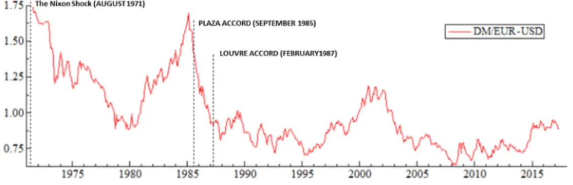
Figure 1- DM/EUR-USD exchange rate from January 1971 to May 2017
Figure 1 shows the time series of the DM/EUR-USD exchange rate from January 1971 to May 2017. The period between September 1985 and February 1987 is characterized by extensive government invention in the currency market. In September 1985 G5 nations (the United States, the United Kingdom, West Germany, France, and Japan) agreed, in the Plaza Accord, to try and generate a depreciation of the United States’ currency against the other 4 nations’ currencies over a two-year period. After this agreement each country’s central bank intervened heavily in the foreign exchange market to reach an agreed-upon undisclosed target rate. This generated a decline in the value of the United States’ currency which reached close to 50%. Subsequently, the Louvre Accord in February 1987 represented an agreement to stop the decline of the dollar and to stabilize G6 nations’ (the G5 plus Canada) currencies. Stability was achieved for the first 8 months after the agreement, but broke down due to an interest rate increase by the German Bundesbank, triggering a rise of the discount rate by the Federal Reserve. Therefore, between these two
7
accords, we expect these policy events to have generated an absence, or a disturbance, of monthly seasonal anomalies in the foreign currency market.
To test the hypothesis of the presence of an overlap in the seasonal pattern of the foreign exchange and stock markets, we use the differential between the returns on the German and the US stock markets. We employ monthly closing quotes of the DAX index17 as the representative of the former and the S&P 500
index as the representative of the latter stock market from February 1971 to May 2017, both obtained from Global Financial Data. The differential is computed as the returns (exclusive of dividends) on the German DAX minus the returns on the S&P 500 (ex. dividends).
To evaluate the channel through which the seasonality in the stock markets could have impacted the foreign exchange market, we investigate the seasonal pattern of the equity flows between Germany and the US. Following Hau and Rey (2006) and Brennan and Cao (1997), we use net equity flows from the US into Germany, which are the net purchases of German stocks by US residents minus the net purchases of US stocks by German residents, normalized on the average of the absolute value of net equity flows from the US to Germany during the previous 12 months. Capital flows between Germany and the US have been reported by the US Department of the Treasury in the Treasury International Capital system (TIC) since January 1977, which is thus the start of the sample used in our study of net equity flows.
Table 1-Descriptive statistics for foreign exchange returns, stock returns differential, and normalized net equity flows
Min Mean Max Standard
deviation Skewness Kurtosis
Jarque-Bera Box-pierce test Q(5) ΔL(DM/EUR-USD) -0.118 -0.001 0.122 0.031 0.08 1.36** 43.23** 3.09 ΔLDAX-ΔLS&P -0.222 0.001 0.184 0.054 -0.25** 1.21*** 39.28*** 10.74* NEF -4.01 -0.06 4.36 1.40 0.152 0.46** 6.30** 110.51*** ADF (1979) Zivot and Andrews (2002) Phillips and Perron (1988) KPSS (1992) Ng and Perron (2001) MZa MZt ΔL(DM/EUR-USD) -12.46*** -11.61*** -22.53*** 0.12 -49.29*** -4.96*** ΔLDAX-ΔLS&P -13.12*** -10.87*** -29.96*** 0.039 -20.64*** -3.19*** NEF -9.01*** -9.19*** -18.38*** 0.25 -70.98*** -5.94***
*** significant at the 1% level, ** significant at the 5% level, * significant at the 10% level
-ΔL(DM/EUR-USD) is the DM/EUR-USD exchange rate return, ΔLDAX-ΔLS&P500 is the returns differential between the German DAX and the US S&P 500 stock indices, NEF is the net equity flows between Germany and the US.
-Sample: February 1971 to May 2017 for the DM/EUR-USD exchange rate returns, March 1971 to May 2017 for the stock market returns differential, and January 1977 to May 2017 for the NEF.
Table 1 shows the descriptive statistics of the exchange rate returns, stock markets returns differentials and net equity flows from the US to Germany. The three variables have non-normal distribution caused by excess kurtosis according to the Jarque-Bera test. All three are stationary according to the Augmented Dickey-Fuller, the Phillips and Perron (1988) and the Kwiatkowski et al. (1992) (KPSS)tests. As these tests are said to be biased towards rejecting the null of unit root (or accepting the null of stationarity in the case of KPSS) in the presence of structural breaks, we also conduct Zivot and Andrews’ (2002) test, which allows for structural breaks, and confirms the stationarity of all variables. A similar confirmation of
17 DAX index was first introduced by the association of the German Stock Exchanges, the Frankfurt Stock Exchange
and the Börsen-Zeitung on July 1, 1988 but is a continuation of the stock market newspaper index which had been reported since 1959.
8
stationarity is provided by Ng and Perron’s (2001) MZa and MZt tests,18 which are modified versions of
Phillips’ (1987) and Phillips and Perron’s (1988) unit root tests.19
Table A1 in the Appendix reports for each month the descriptive statistics of the DM/EUR-USD returns, stock returns differential and normalized net equity flows. On average the USD has the lowest returns vis-à-vis the DM/EUR in Decembers and the highest returns in Januaries. The average of the stock returns differential has the highest value in Februaries and lowest in Mays. The German net equity flows to the US have their lowest mean value in Januaries and highest mean value in Augusts. The monthly data distributions are shown to be non-normal.
2.2 Methodology
The usual parametric and non-parametric tests of equality of means and variances have been extensively used for the detection of seasonality in the literature (see for instance: Gultekin & Gultekin, 1983; Kumar & Pathak, 2016; Lucey & Whelan, 2004; McFarland et al., 1982; Rozeff & Kinney, 1976; Zhang & Jacobsen, 2013 among others). Among these tests the Analysis of Variance (ANOVA) test (Fisher, 1920) and its non-parametric alternative, the Kruskall-Wallis test (Kruskal and Wallis, 1952), focus on the equality of the means of several independent groups, e.g. the average exchange rate return across months in our case. Levene’s test (1960) and its non-parametric counterpart (Nordstokke and Zumbo, 2010) assess the equality of variances of several independent groups (equality of exchange rate variances across months in our case).20
Another parametric test for the detection of monthly anomalies is the usual linear framework which relies on an ordinary least squares (OLS) estimation of a model including 12 monthly dummies (Adrangi and Ghazanfari, 2011; Depenchuk et al., 2010; Floros, 2008; Franses and van Dijk, 2000; Gultekin and Gultekin, 1983; Kumar and Pathak, 2016; Li et al., 2011; Yamori and Kurihara, 2004; Zhang and Jacobsen, 2013) as follows:
𝑀, 𝛽, 𝐷, 𝜀, (1)
where 𝑀, is a monthly series integrated of order 0, with i being either exchange rate returns (MFX,t =
RDM/EUR-USD), the stock market returns differential (MSRD,t) or the net equity flows form the US to Germany
18 By applying GLS de-trending they enhance the power of the tests especially for small samples.
19 Elliott, Rothenberg and Stocks’ (1996) efficient test for autoregressive unit root which is a modified Dickey and
Fullers’ (1979) test could also be implemented. However, in contrast to the trendless nature of our variables, this test is rather proposed for the autoregressive series with a trend component. Therefore, we rather rely on the results of previous tests’ results.
20 ANOVA tests the null of equality of the average value of returns across groups (months) against the alternative of
having at least one group (month) with a different mean (average return) and produces an F-test to conclude. The Kruskall-Wallis non-parametric test uses ranks of data instead of their original values and therefore tests the equality of mean ranks. In contrast to ANOVA, the Kruskall-Wallis non-parametric test does not assume normally distributed data. The test statistic obtained by applying this test is approximately Chi-squared distributed. Levene’s test can be considered as an ANOVA test on the absolute value of each monthly return from the average return of its corresponding group (month) and its test statistic is approximately F-distributed. The non-parametric version of this test uses ranks instead of original values of the observations and consists of an ANOVA test on the absolute value of the difference between the rank of each observation with the average rank of it corresponding group (month).
9
(MNEF,t) in our case. Dj,t is the monthly dummy variable taking value 1 in the jth month (j= 1 to 12) and 0 in other months.21 β
js are the seasonal coefficients which show the average value of the Mi,t series during the corresponding month. Finally, 𝜀, is an iid error terms.
Returns on financial assets (Rl,t ) are calculated as:
𝑅, ln 𝑃,
𝑃 , (2)
with l being the financial asset (foreign currency and stocks) and 𝑃, its spot price. Therefore the stock market returns differential can be computed as (𝑀 , = RDAX,t – RS&p500,t).
An important concern when estimating such a linear model for a long sample is the stability of the parameters, since the seasonal pattern of the exchange rate series may change over time. Given the sophisticated trading technologies, no seasonal anomaly is expected to resist being arbitraged away over time in the globalized currency or stock markets. In addition, government policy changes such as intervention in the market or even cultural changes, such as starting the celebration of holidays (Zhang and Jacobsen, 2013), may affect the seasonal pattern of financial series such as exchange rate or stock returns over time. Therefore, in this study, in order to gauge the modification of the seasonal pattern, we suggest the application of a non-linear specification.
In this context, the use of the Markov-switching model developed by Hamilton (1989) would serve our purpose of modeling the time series which are subject to regime shifts. In contrast with structural break tests, the Markov-switching model allows for the possibility of regime recurrence (Hamilton, 2016). The Markov-switching framework for the detection of seasonal effects of variable M is as follows:
𝑀, 𝛼, 𝑠, 𝑀, 𝛽, 𝑠, 𝐷 𝜎 𝑠, 𝜀, (3)
In equation (1), k (=1 to q) autoregressive lags of 𝑀, are entered as explanatory variables and 𝜀, is Gaussian white noise with covariance matrix Σ. 𝑠, is an unobservable state variable and all the parameters in this model are allowed to switch between states. Therefore, 𝛼, 𝑠, are the state-dependent coefficients of the autoregressive lags, 𝛽, 𝑠, indicates the state-dependent seasonal coefficient of month j and 𝜎 𝑠, is the state-dependent variance.
In this model, the state variable follows a first-order Markov chain, meaning that its current value is affected only by its immediate previous value. Given an information set (data) and a model, we will be able to assign each observation to a specific state. Optimal inference on this unobservable state variable then can yield a matrix of smoothed transition probabilities whose elements show the probability of persistence of a given regime (when starting from that regime) and the probabilities of transition to other regimes. We do not decide a priori about the number of regimes, but test for it. We estimate these parameters using the sequential quadratic programming algorithm of Lawrence and Tits (2001) along with a pre-estimation with the Expected Maximization (EM) algorithm of Dempster, laid and Rubin (Dempster et al., 1977).
21 To avoid the dummy variable trap, this model should not include an intercept, otherwise one of the monthly dummy
10
There are two challenges when specifying a Markov-switching model. The first is that the test-statistics of the usual parameter constancy tests, such as the likelihood ratio test, do not follow standard distributions (Carrasco et al., 2014; Di Sanzo, 2009). This is both because under the null of linearity some of the hyper-parameters are not identified and the information matrix is singular (since the underlying regimes are unobservable). Therefore, in order to test whether a linear model outperforms a non-linear model, we apply the optimal test for Markov-switching proposed by Carrasco et al. (2014). Their test only requires the estimation of the Markov-switching model under the null hypothesis of constant parameters. Therefore, we need only to compute the critical values by parametric bootstrap simulations using our Markov-switching estimation under the null hypothesis (Carrasco et al., 2014). To implement this test for a model with switching intercept and variance, we compute the critical values from 500 iterations.
The second challenge is the choice of the optimal number of regimes. The Akaike (AIC), Bayesian or Schwarz’s (SC) and Hannan and Quinn (1979) (HQ) information criteria are the general metrics used in the literature for comparing the goodness of fit of several models. The three information criteria trade off the log-likelihood obtained from the Markov-switching model against the number of parameters estimated. However, they are all suspected of misleading users to choose an inaccurate number of regimes, the SC and HQ by suggesting models with a low number of regimes (Psaradakis and Spagnolo, 2003) and the AIC by having the tendency to accept a model with a high number of regimes (Smith et al., 2006), leading to the reduction of estimation accuracy.
Therefore, we prefer to conduct our analysis with the Markov-Switching Criterion (MSC), developed by Smith et al. (2006) and based on the Kullback–Leibler (KL) divergence, which allows us to choose simultaneously the optimal number of regimes and autoregressive lags. This criterion was shown to be efficient across different sample sizes and with noisy data (Smith et al., 2006). After the estimation of the model parameters, the MSC is computed by imposing a penalty based on full-sample smoothed probabilities in order to trade off the fit of the model against its parsimony. The criterion is computed as:
𝑀𝑆𝐶 2𝐿 𝜏̂ 𝜏̂ 𝑆𝜂
𝜏̂ 𝑆𝜂 2 (4)
where L is the log-likelihood of the estimated model, S is the number of regimes and η is the number of regressors. 𝜏̂ is defined as the sum of smoothed probabilities of being in the ith regime computed using full-sample smoothed probabilities. The model which yields the minimum MSC is chosen with the optimal number of Markov-switching regimes and autoregressive lags.
In our empirical analysis, we consider various combinations of states (i) and autoregressive lags (k) for the estimation of equation (3). We estimate different models and compute the three information criteria presented above (AIC, SC and MSC). However, the final decision about the best number of regimes and number of autoregressive lags depends on the MSC.
3 Empirical results
To meet the three objectives of our study, we follow a sequential strategy. First, to be able to compare and decide upon the necessity of the application of a non-linear framework, we apply conventional parametric and non-parametric tests. We then examine the monthly seasonality in the foreign exchange market using the non-linear Markov-switching framework. In the next step, we examine the possible drivers of
11
seasonality in foreign currency returns by comparing the timing of its occurrence with the seasonal pattern of the German-US stock returns differential. We then consider whether this similarity in seasonal pattern is matched by the seasonal pattern of bilateral US-German net equity flows.
3.1 Parametric and non-parametric tests of seasonality
The results of the widely-used parametric and non-parametric tests of equality of means and variances of the monthly foreign currency returns, stock returns differential and net equity flows are reported in table 2. None of the tests show any significant difference between monthly means and variances of the stock returns differential. However, conducting the Analysis of Variance (ANOVA) test, a significant difference between monthly means of the DM/EUR-USD exchange rate and also between the means of net equity flows from the US to Germany are found, without indicating the month(s) contributing to the inequality of means (Table 2, second column). The Kruskal-Wallis non-parametric test shows very weak evidence (at the 10% level of confidence) that the mean ranks of monthly returns of the DM/EUR-USD can differ and a strong evidence of differences between monthly means of the net equity flows. Finally, while Levene’s test of equality of variances of the monthly returns differential does not indicate any significant difference in the monthly variances, its non-parametric version shows a difference between the variances of monthly net equity flows.
Table 2- Parametric and non-parametric tests of mean and variance equality
Variable ANOVA test Kruskal-Wallis test Levene’s test Levene’s non-parametric
test MFX 1.871** 17.392* 0.768 1.084 [0.041] [0.097] [0.673] [0.371] MSRD 1.148 0.097 1.439 1.367 [0.322] [0.330] [0.152] [0.184] MNEF 2.1805** 25.485*** 0.715 2.345*** [0.014] [0.007] [0.725] [0.008]
*** significant at the 1% level, ** significant at the 5% level, * significant at the 10% level -Numbers in square brackets are p-values.
-MFX= ΔL(DM/EUR-USD): DM/EUR-USD exchange rate return, MSRD=ΔLDAX-ΔLS&P500: stock markets returns differential, MNEF: net equity flow form the US to Germany.
-Sample: February 1971 to May 2017 for the DM/EUR-USD exchange rate returns, March 1971 to May 2017 for the stock market returns differential, and January 1977 to May 2017 for the net equity flows from the US to Germany.
A linear model with monthly dummies as in equation (1) was estimated as a starting point. The results, reported in table 3, show that significant January, September and December effects exist in the DM/EUR-USD foreign exchange returns. However, the results of the estimation of the linear model for the stock returns differential only reveal the presence of a significant February effect. Hence, the hypothesis of the presence of a January effect in the stock markets returns differential is rejected using the linear estimation. Accordingly, based on the results of the estimation of such linear specifications, we conclude that there is no similarity between the seasonality in the foreign exchange and stock markets. For the net equity flows, several months such as January, August, October and November have significant coefficients. So, according to the linear estimation, the January effect is only common between the DM/EUR-USD returns and the net equity flows. However, the reliability of such results depends on the validity of the linearity assumption.
12
Table 3- Linear model estimation for foreign exchange returns, stock returns differential and normalized net equity flows
Dependent variables Jan Feb Mar Apr May Jun
MFX 0.011** -0.004 0.001 -0.003 0.006 -0.003 [0.02] [0.31] [0.82] [0.40] [0.16] [0.49] MSRD -0.008 0.014* 0.002 0.001 -0.012 0.003 [0.29] [0.07] [0.79] [0.85] [0.12] [0.66] MNEF -0.501** -0.152 -0.331 0.028 0.042 0.272 [0.02] [0.48] [0.13] [0.90] [0.85] [0.22]
Dependent variables Jul Aug Sep Oct Nov Dec
MFX -0.002 0.001 -0.010** -0.003 0.003 -0.011** [0.66] [0.86] [0.02] [0.59] [0.60] [0.01] MSRD 0.013 -0.010 -0.005 0.006 0.004 0.007 [0.11] [0.21] [0.57] [0.48] [0.64] [0.40] MNEF 0.128 0.524** 0.263 -0.389* -0.476** -0.028 [0.56] [0.02] [0.23] [0.08] [0.03] [0.90]
*** significant at the 1% level, ** significant at the 5% level, * significant at the 10% level -Numbers in square brackets are p-values.
-MFX= ΔL(DM/EUR-USD): DM/EUR-USD exchange rate return, MSRD=ΔLDAX-ΔLS&P500: stock markets returns differential, MNEF: net equity flow from the US to Germany.
-Sample: February 1971 to May 2017 for the DM/EUR-USD exchange rate returns, March 1971 to May 2017 for the stock market returns differential, and January 1977 to May 2017 for the net equity flows from the US to Germany.
3.2 Markov-switching estimation results 3.2.1 Linear model vs. Markov-switching
To make sure that a regime-switching model is relevant for our data, we first implement the optimal test for the constancy of parameters. We implement Carrasco et al. (2014)’s test of linearity vs. Markov Switching mean and variance separately for the DM/EUR-USD exchange rate returns, the German-US stock market returns differential, and the net equity flows from the US to Germany, using 500 iterations. The results obtained from these tests are provided in Table 4, where SupTS is a sup-type test statistic used by Davies (1987) and expTS is an exponential-type test statistic suggested by Andrews and Ploberger (1994).
Table 4- Carrasco et al (2014)’s test of linearity vs. Markov-switching model with switching mean and variance
supTS expTS
MFX 9.356 [0.00] 14.00 [0.00]
MSRD 12.582 [0.00] 8.076 [0.00]
MNEF 9.480 [0.00] 75.807 [0.00]
-MFX= ΔL(DM/EUR-USD): DM/EUR-USD exchange rate return, MSRD=ΔLDAX-ΔLS&P 500: stock markets returns differential, MNEF: net equity flow from the US to Germany.
-Numbers in square brackets are p-values.
-Sample: February 1971 to May 2017 for the DM/EUR-USD exchange rate returns, March 1971 to May 2017 for the stock market returns differential, and January 1977 to May 2017 for the net equity flows from the US to Germany.
The results (table 4) show that the null of a linear model against a model with switching mean and variance is strongly rejected for all three variables. Therefore, the results of the linear model with 12 monthly dummy variables and the conventional parametric tests are not acceptable and we should instead rely on a non-linear model such as the Markov-switching model.
13
3.2.2 Foreign exchange market
To choose the optimal number of regimes of the non-linear model of exchange rate returns, we estimated 18 models with i=2 to 4 regimes and k=0 to 5 autoregressive lags in which all the components of equation (3) were allowed to be regime dependent. We do not go further than 4 regimes because our model would be over-parametrized. The period of estimation is from July 1971 to May 2017, as we reserved the first observation for the computation of the returns from the spot prices and the next 5 observations for the inclusion of autoregressive lags. Columns 3 to 5 of table 5 report the obtained values for the three information criteria for the 18 models with DM/EUR-USD returns as the dependent variable. AIC suggests a model with 4 regimes and 5 autoregressive lags, while a model with 2 regimes and no autoregressive lag is suggested by SC. The lowest MSC is obtained by a 3-regime model with 4 autoregressive lags. So, as we expected, MSC favors fewer regimes in comparison with AIC and a larger number of regimes in comparison with SC.
Table 5- Information criteria obtained from estimated MS models for DM/EUR-USD exchange rate returns, stock market returns differential and the net equity flows from the US to Germany
Info. MFX MSRD MNEF
Criterion i=2 i=3 i=4 i=2 i=3 i=4 i=2 i=3
k=5 MSC -1604.380 -1117.020 -1651.600 -1131.712 -1019.463 -887.061 2158.641 2478.355 SC -3.787 -3.648 -3.596 -2.746 -2.539 -2.375 3.544 3.638 AIC -4.085 -4.102 -4.230 -3.043 -3.001 -3.002 -794.932 3.307 k=4 MSC -1608.960 -3314.620 -1749.490 -1123.390 -1044.230 -514.743 2148.387 2426.162 SC -3.784 -3.707 -3.692 -2.731 -2.556 -2.559 3.536 3.613 AIC -4.066 -4.137 -4.295 -3.013 -3.003 -3.163 3.388 3.300 k=3 MSC -1618.830 -2389.480 -1716.540 -1129.680 No conv. No conv. 2137.354 2379.772 SC -3.807 -3.658 -3.572 -2.749 No conv. No conv. 3.524 3.588
AIC -4.073 -4.081 -4.127 -3.016 No conv. No conv. 3.385 3.292
k=2 MSC -1628.260 -903.649 -1846.320 -1136.620 -1098.690 -962.557 2127.777 2341.900 SC -3.827 -3.758 -3.612 -2.769 -2.601 -2.615 3.520 3.565 AIC -4.078 -4.141 -4.144 -3.020 -2.993 -3.140 3.389 3.287 k=1 MSC -1638.130 -1045.910 -1671.200 -1145.920 -1151.080 -1099.670 1995.593 2311.427 SC -3.850 -3.710 -3.683 -2.793 -2.704 -2.498 3.556 3.557 AIC -4.085 -4.078 -4.168 -3.028 -3.064 -3.000 3.434 3.296 k=0 MSC -1633.860 -1361.240 -2200.400 -1141.760 No conv. -1188.415 2169.252 2281.744 SC -3.885 -3.750 -3.622 -2.792 No conv. -2.667 3.626 3.626 AIC -4.104 -4.086 -4.107 -3.011 No conv. -3.137 3.513 3.382
-MFX= ΔL(DM/EUR-USD): DM/EUR-USD exchange rate return, MSRD=ΔLDAX-ΔLS&P500: stock markets returns differential, MNEF: net equity flow from the US to Germany.
- k: number of Autoregressive lags, i: number of regimes.
- Sample: July 1971 to May 2017 for the DM/EUR-USD exchange rate returns, August 1971 to May 2017 for the stock market returns differential, and June 1977 to May 2017 for the net equity flows from the US to Germany.
- No Conv. indicates that the maximization algorithm does not converge. Therefore, we neglect the models which do not converge in our model comparison.
14
The estimated coefficients for a 3-regime model with 4 autoregressive lags, suggested by MSC, are presented in table 6. Regime switches have taken place in association with changes in the variance of the error terms, the seasonal pattern and the autoregressive terms. The first regime is the most persistent or dominant (the probability of its persistence is 97%), and the second regime is the least persistent (see figure 2). The third regime is the high-volatility regime, and the second one is the low-volatility regime (refer to table A2 in the Appendix for regime transition probabilities).
Table 6- Markov-switching estimated coefficients of DM/EUR-USD exchange rate returns (July 1971-May 2017)
Regime Jan Feb Mar Apr May Jun
1 0.016*** -0.005 0.001 0.001 0.006 -0.002 (0.004) (0.004) (0.004) (0.004) (0.005) (0.004) 2 -0.058*** -0.028*** -0.042*** -0.034*** -0.002 -0.010*** (0.003) (0.004) (0.003) (0.004) (0.003) (0.003) 3 -0.002 -0.027 0.099*** -0.017 0.008 -0.009 (0.018) (0.017) (0.028) (0.017) (0.019) (0.016)
Regime Jul Aug Sep Oct Nov Dec
1 0.004 -0.005 -0.006 -0.001 0.004 -0.008* (0.004) (0.005) (0.005) (0.004) (0.005) (0.004) 2 0.003 -0.007*** -0.044*** -0.011*** -0.042*** -0.048*** (0.002) (0.002) (0.002) (0.002) (0.006) (0.003) 3 -0.060*** 0.020 -0.015 0.002 0.049 -0.011 (0.021) (0.017) (0.018) (0.020) (0.030) (0.023)
Regime MFX(-1) MFX(-2) MFX(-3) MFX(-4) variance prob. of
persistence 1 0.170*** -0.005 0.013 -0.051 0.025*** 0.976 (0.051) (0.049) (0.047) (0.045) (0.001) (0.008) 2 -0.390*** -0.269*** -0.261*** -0.150*** 0.004*** 0.503 (0.020) (0.017) (0.020) (0.018) (0.001) (0.093) 3 -0.079 0.310* 0.218 0.473*** 0.039*** 0.668 (0.118) (0.144) (0.145) (0.161) (0.003) (0.071)
Portmanteau (36) 18.986 Normality test 2.5956 ARCH test 0.19560
*** significant at the 1% level, ** significant at the 5% level, * significant at the 10% level - Numbers in parentheses are standard errors.
- MFX= ΔL(DM/EUR-USD): DM/EUR-USD returns.
- Coefficients in this table should be read as this example: 0.016 in January means a 1.6% exchange rate return.
During the first regime, the only significant coefficients are the ones corresponding to January (significant at the 1% level) with an average return of 1.6 percentage points (0.016) and December (significant at the 10% level) with an average return of -0.8 percentage points (-0.008). Therefore, we cannot reject the hypothesis that the January and December effects are present for the DM/EUR-USD exchange rate during the most persistent regime. As shown in figure 2 and table A3 of the Appendix for the regime classifications, the first regime still has many occurrences in the most recent period. Accordingly, the end/beginning of the year seasonal anomaly of the DM/EUR-USD exchange rate returns is not an obsolete phenomenon. Therefore, market participants have not been able to gradually smooth it out (or arbitrage it away). The January (December) effect here corresponds to an appreciation (depreciation) of the US dollar vis-à-vis the DM/EUR.
15
During the second regime, which is the least persistent one, we have 10 significant monthly coefficients. This regime is in place in only less than 10% of the whole sample. Similarly, the third regime is only in place in 67 out of 552 months (12% of the whole sample) and only coefficients corresponding to March, April and July are significant. Having few observations in a regime (like here the second and third ones) can generate the statistical significance of many coefficients, which cannot be interpreted as the presence of the month effect in those regimes. Interestingly, the period between the Plaza and Louvre accords plus the first three months after the Louvre accord (September 1985 to April 1987) fall into the second and third regimes (total of 20 months). This is in accordance with our expectation of no monthly seasonal pattern when governments intervene in the market.
With the application of the Markov-switching framework, we are thus able to document the presence of the January and December effects in the DM/EUR-USD exchange rate returns. These effects either were not identified in previous papers (Cellini and Cuccia, 2011) or were only modeled in a linear framework (Li et al., 2011) and with a much shorter sample (Cellini and Cuccia, 2014). As opposed to the results using a linear OLS framework, we do not find any significant evidence of a monthly anomaly in September. To show that this finding of month effects in the foreign exchange market is not simply a statistical anomaly but is also exploitable for trading, we must make sure that the transaction costs do not exceed the profit from the arbitrage transactions. The most common form of transaction costs in the foreign exchange market is the bid-ask spread. Since October 1989, the variable bid-ask spreads of the DM/EUR-USD exchange rate have usually been so small (on average 1 pip) that all the transactions involved in arbitraging the January effect in the foreign currency market remain profitable net of the spread (table A4 in the Appendix). We also show in the Appendix that the profit net of the spread is high enough to be larger than any fixed or variable transaction fees.22
Figure 2-Smoothed regime probabilities of the DM/EUR-USD exchange rate returns
22 Transaction fees (bid-ask spreads) are omitted from the return made from the appreciation of the US dollar (German
16
3.2.3 Stock market
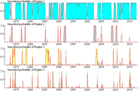
With respect to the returns differential between the German and US stock markets (DAX and S&P 500 respectively), we use the same procedure as for exchange rate returns, estimating 18 models with i=2 to 4 and k=0 to 5. We do not go further than 4 regimes because our model would be over-parametrized. We reserve the first 6 observations for autoregressive lags and differencing. Therefore our estimation sample is from August 1971 to May 2017. As shown in table 5, the model suggested by MSC has 4 regimes, with no autoregressive lags. Estimated coefficients are reported in table 7. Similar to the case of the DM/EUR-USD exchange rate returns, the first regime is dominant and the three other regimes have short durations and are very seldom in place (9.45% of the whole sample for the second and third regimes and 4.18% for the fourth regime) (see Fig. 3). With the same reasoning as for (in)significant coefficients in the second and the third regimes of the model for the exchange rate returns, we reject the presence of a monthly seasonal pattern in the last three regimes of the model for the stock market returns differential.
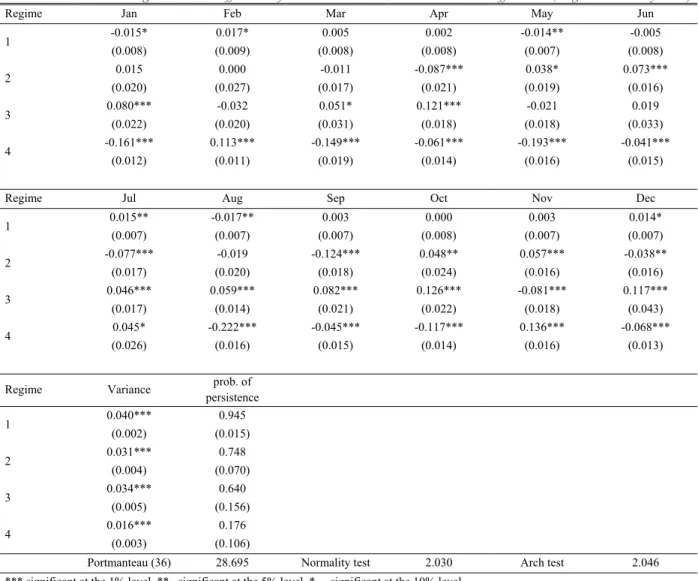
Table 7- Markov-switching estimated coefficients of the German-US stock market returns differential (August 1971- May 2017)
Regime Jan Feb Mar Apr May Jun
1 -0.015* 0.017* 0.005 0.002 -0.014** -0.005 (0.008) (0.009) (0.008) (0.008) (0.007) (0.008) 2 0.015 0.000 -0.011 -0.087*** 0.038* 0.073*** (0.020) (0.027) (0.017) (0.021) (0.019) (0.016) 3 0.080*** -0.032 0.051* 0.121*** -0.021 0.019 (0.022) (0.020) (0.031) (0.018) (0.018) (0.033) 4 -0.161*** 0.113*** -0.149*** -0.061*** -0.193*** -0.041*** (0.012) (0.011) (0.019) (0.014) (0.016) (0.015)
Regime Jul Aug Sep Oct Nov Dec
1 0.015** -0.017** 0.003 0.000 0.003 0.014* (0.007) (0.007) (0.007) (0.008) (0.007) (0.007) 2 -0.077*** -0.019 -0.124*** 0.048** 0.057*** -0.038** (0.017) (0.020) (0.018) (0.024) (0.016) (0.016) 3 0.046*** 0.059*** 0.082*** 0.126*** -0.081*** 0.117*** (0.017) (0.014) (0.021) (0.022) (0.018) (0.043) 4 0.045* -0.222*** -0.045*** -0.117*** 0.136*** -0.068*** (0.026) (0.016) (0.015) (0.014) (0.016) (0.013)
Regime Variance prob. of
persistence 1 0.040*** 0.945 (0.002) (0.015) 2 0.031*** 0.748 (0.004) (0.070) 3 0.034*** 0.640 (0.005) (0.156) 4 0.016*** 0.176 (0.003) (0.106)
Portmanteau (36) 28.695 Normality test 2.030 Arch test 2.046
*** significant at the 1% level, ** significant at the 5% level, * significant at the 10% level -Numbers in square brackets are standard errors.
-Coefficients in this table should be read as this example: -0.015 in January means that during that month US stock returns are 1.5 percentage points higher than the German stock returns.
17
In the first regime, which is dominant and highly-volatile, we find significant coefficients for January, February, May, July, August and December (refer to tables A5 and A6 of the Appendix for regime transition probabilities and the dating of regimes). In that regime, the coefficient of the January dummy is almost equal to, but with an opposite sign from, the coefficient of the December and February dummies. In Januaries (December and February respectively) US stock returns are 1.5 (1.4 and 1.7 respectively) percentage points higher (lower) than German stock returns. This double reversal can provide an equity carry trade opportunity to investors who not only benefit from the stock market returns differential, but also take advantage of currency movements during December and January. Therefore, adding up the returns from the foreign exchange market and stock returns differential, an investor who would have moved her capital to the German (US) stock market in December (January) would have benefited from an overall gross return in excess of 2.0 (3.0) percentage points (if both the foreign exchange rate returns and stock returns differential lie in their seasonality regimes).
Figure 3- Smoothed regime probabilities of the (German-US) stock market returns differential
3.2.4 Similar January effect in the foreign exchange market returns and the stock market returns differential
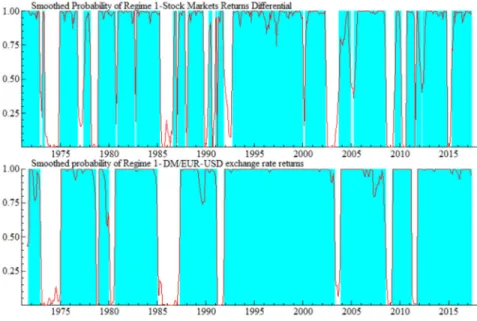
The first regime of the model for the DM/EUR-USD exchange rate returns and the first regime of the stock market returns differential have similar timings, as shown respectively in the lower and upper panels of figure 4. More specifically, since August 1971, the DM/EUR-USD exchange rate returns fall in the first regime for a total of 431 months. As shown in table 8, 368 out of these 431 months correspond also to the first regime of the stock market returns differential. In other words, there are only 62 months that are classified in the first regime of the DM/EUR-USD exchange rate return model but not in the first regime of the stock markets returns differential. Conversely, there are 54 month that are classified in the first regime of the model for the stock markets returns differential but not in the model for DM/EUR-USD exchange rate returns.
This considerable overlap of the January and December effects is a presumption of the presence of a similar seasonality in the two markets. The negative (positive) sign of the coefficient of January (December and
18
February) in the first regime of the model for the stock returns differential, which indicates the presence of an incentive for investors to switch a part of their portfolio from the German (US) to the US (German) stock market during the corresponding month, is accompanied by an appreciation (depreciation) of the dollar in Januaries (Decembers but not Februaries). Therefore, it is likely that the January and December effects in the DM/EUR-USD exchange rate returns are associated with the significant differential between the returns of the US and the German stock markets in Januaries and Decembers. In other words, in Januaries investors tend to sell German stocks quoted in euros (or DM prior to formation of the euro) and to use the proceeds to buy USD in order to invest in the American stock market (and vice versa in Decembers). This shows that during the similar-seasonality period Hau and Rey (2006)’s UEP does not hold between contemporaneous values of exchange rate returns and stock returns differential, meaning that the stock returns differential is not compensated immediately by the depreciation of the USD. However, in a one month horizon this parity condition is vindicated. The induced cross-border capital flows transiting via the foreign currency market are likely to be the source of the similar seasonality in the stock market returns differential and the foreign exchange returns.
Figure 4-Smoothed regime probabilities of the first regimes of the (German-US) stock returns differential (upper panel) and the DM/EUR-USD exchange rate returns (lower panel)
There are still a few years when the January effect is absent from both the DM/EUR-USD returns and the stock returns differential. We can explore the common causes of the elimination of this seasonal anomaly during three episodes. First, the first oil shock, in early autumn 1973, seems to have caused the returns differential of the two stock markets to temporarily switch from its high-volatility dominant state to another state for a period of one year. However, we do not see such an effect following the second oil shock, in December 1979. Therefore, we may instead interpret the 1973-74 specificity as the effect of temporary capital controls, such as the prohibition of interest payments on non-resident deposits until 1975 in Germany.23 Second, the effect of the controls on capital inflows into Germany can be also observed during
the years 1977 and 1979, when both the DM/EUR-USD exchange rate returns and the stock market returns
23 Refer to the IMF Annual Reports on Exchange Arrangement and Exchange Restrictions available on
19
differential are out of their dominant regimes. Finally, the period between 1985 and 1987 does not lie in the first regime of the foreign currency returns, thus showing no January and December effects. This was the period between the Plaza and Louvre accords (see above), characterized by heavy interventions in the foreign exchange market aimed at managing an orderly depreciation of the US dollar vis-à-vis the G5 nations’ currencies. Therefore, not only we do not observe any January and December effects in the DM/EUR-USD during this period, but also a more persistent January effect in the German-US stock returns differential could have been prevented due to expectations of the depreciation of the USD.
The period from mid-2002 to mid-2003 marks sharp downturn in the US and European stock markets known as the burst of the internet bubble. As it is expected for turmoil periods, our estimations show that the DM/EUR-USD returns and the stock returns differentials do not stand in their dominant regimes. The stock returns differential lies in its second regime, with relatively-low volatility, and the EUR-USD bounces between its most- and least-volatile regimes. The Global Financial Crisis caused a similar elimination of the January and December effects from mid-2008 to mid-2009.
Table 8- Timing of joint seasonality between DM/EUR-USD exchange rate returns and the (German-US) stock returns differential (Aug 1971-May 2017)
Joint seasonality Months Classified only the 1st regime of in MFX
Months Classified only the 1st regime of MSRD Months 1971(08)- 1971(11) 4 1971(12) 1 1973 (03)- 1973(05) 2 1972(01)- 1972(11) 11 1972(12) 1 1974(12) 1 1975(02)- 1976(10) 21 1976(11)- 1977(05) 7 1978(10) 1 1977(06)- 1978(02) 9 1978(03)- 1978(09) 7 1979(10)- 1979(11) 2 1979(01)- 1979(09) 9 1980(11)- 1980(12) 2 1980(01)- 1980(08) 8 1979(12) 1 1982(10) 1 1985(02)- 1985(04) 3 1980(9) 1 1987(12)- 1988(02) 3 1986(09)- 1986(12) 4 1980(12)- 1982(09) 10 1989(12)- 1990(04) 5 1987(03)- 1987(04) 2 1982(11)- 1985(01) 27 1990(09)- 1990(12) 4 1989(05)- 1989(10) 6 1987(05)- 1987(11) 7 1991(12)- 1992(09) 10 1991(04)- 1991(11) 8 1988(03)- 1989(04) 14 2002(06)- 2002(11) 6 2003(10)- 2003(11) 2 1990(05)- 1990(08) 4 2003(10)- 2003(11) 2 2010 (09)- 2010(12) 4 1991(01)- 1991(02) 2 2005(01)- 2005(02) 2 2011(01)- 2011(07) 7 1992(10)- 2000(01) 88 2005(04) 1 2011(09)- 2011(10) 2 2000(04)- 2002(05) 26 2009(04)- 2009(06) 3 2003(12)- 2004(12) 13 2010(03)- 2010(04) 2 2005(03) 1 2012( 04) 1 2005(05)- 2008(07) 39 2014(12)- 2015(04) 5 2009(07)- 2010(02) 8 2011(01)- 2011(02) 2 2011(11)- 2012(03) 5 2012(05)- 2014(11) 31 2015(05)- 2017(05) 25 Total 368 62 54
-MFX= ΔL(DM/EUR-USD): DM/EUR-USD exchange rate return, MSRD=ΔLDAX-ΔLS&P500: German/US stock markets returns differential.
Overall, combining the probabilities of regimes and average returns in each regime for both foreign currency returns and the stock returns differential, we can infer that an investor selling her US equities in December in order to purchase the German currency and equities would have made on average a 2.6% total gross monthly return. The opposite transactions would have generated a 1.7% total gross monthly return in
20
January, and similar transactions in February as the end of the year would have generated a 2% total gross gain. The overall gross gain over three months would thus be 6.4%, and the net gain would likely be more than 4%, when accounting for bid-ask spreads and fees on the three markets (the US and German stock and the foreign exchange markets). As a point of comparison, it is instructive to note that an investor who would have conducted the same investment strategies in a systematic way every year (from December 1971 to February 2017) would have made on average a gross capital gain of 1.82 % in December, 1.93% in January, and 1.82% in February, computed using the actual average returns by month as reported in table A1. The overall gross gain (5.63%) would thus be close to that implied by our model estimates.
3.2.5 Seasonal carry trade
A valid concern about the seasonality we found in the foreign exchange market returns and its linkage to the seasonality in the stock market returns differential is the effect of regulatory barriers on the mobility of capital. Capital controls, which were at the heart of the Bretton-Woods system, were gradually abolished in the 1970s and 1980s in European countries. As mentioned earlier, in the case of Germany, which was the most liberal European country in this sense, controls on capital outflows were relaxed very early on, in 1957. However, some inflow restrictions were still in place during the 1960s and early 1970s. Subsequently, during the years 1968 to 1973 and 1977 to 1978, different types of controls with varying degrees of severity were imposed again on capital inflows into Germany. In addition, interest payments to non-residents were prohibited until 1975.24 Subsequently, European countries, led by Germany, started to relax their capital
controls. Within the Single Market program EU countries had to fully lift such controls by July 1st 1990.
In order to assess the impact of capital controls of varying intensity on currency returns’ seasonal anomalies one may be tempted to look at reports on the regulations of capital movements as compiled by the International Monetary Fund. However this would not in any way inform us on the actual effectiveness of such controls, which are likely to have been sidestepped in a country with a very open trade account (see Aizenman (2009)), such as Germany. The acid test of such effectiveness is the magnitude of bilateral capital flows, in our case between Germany and the United States. Therefore, we use US-German net equity flows as described in section 2. We were not able to use the capital flow data between the Euro area and the US as the time span for such data is very short. Further, studying aggregate euro-area equity flows would introduce some nuisance into our analysis, as Germany is the main financial actor in the area.
Accordingly, we estimate the MS equation (3) for the bilateral net equity flows from the US into Germany using 12 monthly dummy variables for the sample from June 1977 to May 2017 (for the sake of comparison between models with different number of autoregressive lags, the first 5 observations were omitted). We did not allow more than 3 regimes to preserve degrees of freedom and avoid over-parameterization. By applying the same procedure as in the previous sections, we find that a model with 2 regimes and one autoregressive lag is supported by MSC (refer to table 5 for the comparison of the information criteria obtained by the estimation of the 10 models, and to table A7 of the Appendix for the regime classification of the selected model). Fig. 5 shows the smoothed regime probabilities of this model.
As shown in table 9, the net US equity flows into Germany exhibit seasonal movements. We observe strong January, October, November and December effects in the second regime, which is the dominant (in place
24 Refer to Ghosh and Qureshi (2016) for a brief presentation of the capital controls in Germany and the IMF Annual
21
in more than 64% of the total time) and the least-volatile regime. During the first regime strong June and August effects and a weak April effect are present. The negative sign of the seasonal dummy in January, October and November (in regime 2) implies that during these months capital was flowing from Germany to the US and in the opposite direction during December. The timing of the second regime of the net equity flows has major overlaps with the timings of the first regime of the two models for the exchange rate returns and the stock market returns differential. The discrepancies are prominent in the mid-1980s, between the Plaza and Louvre accords, when we do not observe any January effect either in foreign exchange returns or in the stock market return differentials, while this effect is significant in the US net equity flows into Germany. The discrepancies during more recent years may be explained by the influence of other types of bilateral capital flows (government or corporate bonds, as well as bank flows, etc.) on the foreign exchange returns. In total, the stock market returns are significantly higher in the US than in Germany in 31 out of the 40 Januaries in our sample (from 1977 to 2017) and the net equity flows also exhibit seasonality in 20 Januaries. Finally, an overlapping seasonality is found in stock market returns differential, exchange rate returns and the net equity flows during 18 Januaries.
Figure 5- Smoothed regime probabilities of the net equity flows- whole sample (June 1977-May 2017)
A very important feature of the seasonal pattern in all three (stock market, foreign currency market and net equity flow) models is the significant December and January coefficients that have opposite signs. This common pattern can be regarded as an evidence of carry trade reversal. The equity capital that generally seems to flow from the US to Germany in December for return-chasing purposes subsequently would flow back to the US in order to gain from the larger January effect in the US than in the German stock Market. Such inverse flows would cause significant and consistent movements in foreign exchange returns both in January and December. These patterns match the argument of Curcuru et al (2014), who suggest that the rationale behind the link between the stock market returns differential and foreign exchange returns may not be due to risk balancing and repatriation of investments (suggested by UEP of Hau and Rey (2006)) but to carry trades and the return-chasing behavior of investors. Our findings also suggest that carry trades can be regarded as a seasonal phenomenon which can regularly be present for decades. There is no evidence of a carry trade reversal in February. It is not possible to judge, using the net equity flow data, whether the equity capital that flows from Germany to the US during January is invested there for a relatively longer horizon (a few months), or if investors rebalance their portfolio later in the year to chase returns in third