Computational methods for non-planar vortex wake flow fields with applications to conventional and rotating wings

Applications to Conventional and Rotating Wings

by

Paul Michael Stremel

B.S. Aerospace Engineering, University of Colorado (1977)

SUBMITTED TO THE DEPARTMENT OF AERONAUTICS AND ASTRONAUTICS IN PARTIAL FULFILLMENT OF THE

REQUIREMENTS OF THE DEGREE OF

MASTER OF SCIENCE IN AERONAUTICS AND ASTRONAUTICS

at the

MASSACHUSETTS INSTITUTE OF TECHNOLOGY February 1982

Massachusetts Institute of Technology 1982

Signature of Author /

Department of Aeronautics and Astronautics Certified by Earll M. Murman Thesis Supervisor Accepted by Harold Y. Wachman Chairman, Department Graduate Committee

Archhe

OF TECHNOLOGY L LwL

_{2 5198 2}

COMPUTATIONAL METHODS FOR NON-PLANAR VORTEX WAKE FLOW FIELDS WITH APPLICATIONS

TO

CONVENTIONAL AND ROTATING WINGS by

Paul Michael Stremel

Submitted to the Department of Aeronautics and Astronautics on February 1, 1982 in partial

fulfillment of the

requirements for the Degree of M'aster of Science in Aeronautics and Astronautics

ABSTRACT

Newly developed techniques for the computation of non-planar vortex flow fields are presented. These techniques are designed to track point vortices in an incompressible, inviscid and irrotational fluid. In this method, the point vortices are tracked by Lagrangian methods while the flow field velocity, induced by the singularities, is calculated on an Eulerian mesh. This technique is termed the Eulerian-Lagrangian Method. Solutions to non-planar vortex wake flow fields for conventional wings are obtained by representing the flow field as a two-dimensional time

dependent problem. Calculations are conducted on the Trefftz plane. Solutions to non-planar vortex wake flow fields for rotating wings are obtained from a two-dimensional model of the three-dimensional rotor wake. Calculations are conducted on an Eulerian mesh for the rotating wing analysis. The

point vortices defining the vortex sheet are redistributed on the Eulerian mesh by use of the "Cloud in Cell" technique.

Calculations representing conventional and rotating wing load distributions are presented. In particular, the rollup of the vortex wake generated by an elliptically loaded wing and the wake for a load distribution simulating a wing with a deflected flap are included. The rollup of the vortex wake for a rotating wing in the hover condition is shown. Results of computational experiments to determine the effects of grid size, number of vortex points in the wake definition

and type of singularity representation (constant circulation strength or constant incremental spacing along the span) are presented.

Results indicate the ability of the method to calculate vortex flow fields consisting of single vortex wakes with one or several rolled up vortex cores and flow fields consisting of numerous wake representations, each containing several vortex cores. Predicted locations of the rolled up vortex cores are compared with the theoretical results of Betz and have been found to be in close agreement for an elliptical

load distribution. Predictions of the location and structure of the wake for a rotating wing in hover are compared and contrasted with the findinas of Miller [19].

Thesis Supervisor: Dr. Earll M. Murman

ACKNOWLEDGEMENTS

Special expressions of gratitude are extended to

Professor E. M. Murman for his continual g'iidance, enthusiasm and confidence. Always, when times seemed darkest, Professor Murman provided inspiration to continue.

I would also like to thank Professor R.H. Miller for his many hours spent discussing the characteristics of rotating wing flow fields.

Special thanks to Marilyn Evans for her efficient typing of this manuscript and especially for her patience and

understanding.

TABLE OF CONTENTS SECTION PAGE Abstract 2 Acknowledgements 4 List of Illustrations 7 List of Symbols 11 1. Introduction 13

1.1 Importance of Non-planar Vortex Wake Analysis 13

1.2 Previous Investigations 15

1.2.1 Vortex Flows and Conventional Wings 15

1.2.2 Rotating Wings 19 1.3 Current Investigation 22 1.3.1 Conventional Wings 23 1.3.2 Rotating Wings 26 2. Formulation of Problem 32 2.1 Governing Equations 33 2.1.1 Conventional Wings 33 2.1.2 Rotating Wings 35 2.1.3 Betz's Approximations 38

2.2 Dimensionless Forms of the Equations 39

2.2.1 Conventional Wings 39

2.2.2 Rotating Wings 41

2.3 Single Value Restrictions on the Velocity 43 Potential

3. Numerical Scheme 46

3.1 Finite Difference Forms of the Equations 46 3.2 "Cloud in Cell" Redistribution Scheme 52

3.3 Numerical Solution 54

3.4 Accuracy, Stability 58

4. Computational Experiments 61

4.1 Conventional Wings - Elliptical Load 61 Distribution

4.1.1 Input Description 61

4.1.2 Input and Mesh Variations 63

4.2 Conventional Wings - Deflected Flap 67

4.2.1 Input Description 67

4.2.2 Input and Mesh Variations 69

4.3 Rotating Wings 73

4.3.1 Input Description 73

4.3.2 Results 75

SECTION PAGE

References 79

Illustrations 82

Appendices

A. Single Value Restrictions on the Velocity 167 Potential

A.1 Jump Conditions 167

A.2 Finite -Difference and Non-dimensional 171 Forms

B. Redistribution of Point Singularities 175 C. Rotating Wing - Intermediate and Far Wake 179

Models

LIST OF ILLUSTRATIONS

FIGURE PAGE

1.1 Computational Plane Representation 82 1.2 Betz Approximations to Rotating Wing Load 83

Distributions

1.3 Far Wake Models for Rotating Wing Analysis 84 (Miller)

1.4 Flow Chart - Conventional Wing Analysis 85 1.5 Computational Plane Representation for Rotating 86

Wing Analysis

1.6 Intermediate and Far Wake Models 87

1.7 Geometry of Input - Rotating Wing 88 1.8 Flow Chart - Rotating Wing Analysis 89 2.1 Schematic of Boundary Condition on the Velocity 90

Potential

2.2 Donaldson's Method for Rolled Up Vortex Cores 91 4.1 Wing Loading and Shed Wake Strength - Elliptically 92

Loaded Wing

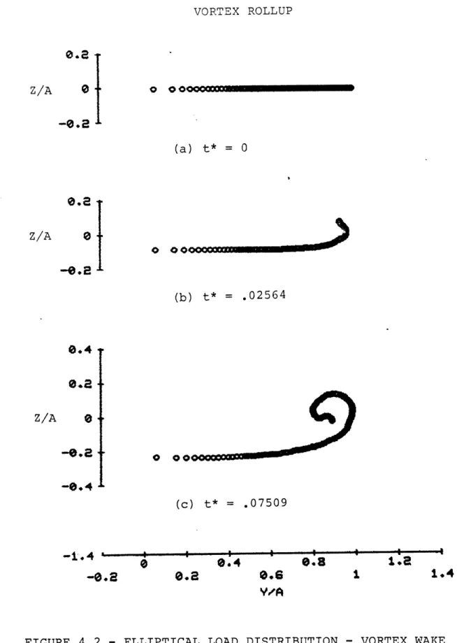
4.2 Elliptical Load Distribution - Vortex Wake 93 Geometry, Constant Strength Point Vortices,

120 Points, Grid = 31x31 4.2a t* = 0 93 4.2b t* = .02564 93 4.2c t* = .07509 93 4.2d t* = .15730 94 4.2e t* = .25590 94 4.2f t* = .36168 95

4.3 Elliptical Load Distribution - V Velocity Profile, 96 Constant Strength Point Vortices, 120 Points,

Grid = 31x31

4.3a t* = 0 96

4.3b t* = .36168 97

4.4 Elliptical Load Distribution - W Velocity Profile, 98 Constant Strength Point Vortices, 120 Points,

Grid = 31x31

4.4a t* = 0 98

4.4b t* = .36168 99

4.5 Elliptical Load Distribution - Vortex Wake 100 Geometry Equally Spaced Point Vortices, 120 Points,

Grid = 31x31 4.5a t* = 0 100 4.5b t* = .02542 100 4.5c t* = .08067 100 4.5d t* = .15537 101 4.5e t* = .25381 101 4.5f t* = .35863 102 4.5g t* = 1.01033 103

PAGE 4.6 Elliptical Load Distribution - V Velocity Profile, 104

Equally Spaced Point Vortices, 120 Points,

Grid = 31x31

4.6a t* = 0 104

4.6b t* = .35863 105

4.7 Elliptical Load Distribution - W Velocity Profile, 106 Equally Spaced Point Vortices, 120 Points,

Grid = 31x31

4.7a t* = 0 106

4.7b t* = .35863 107

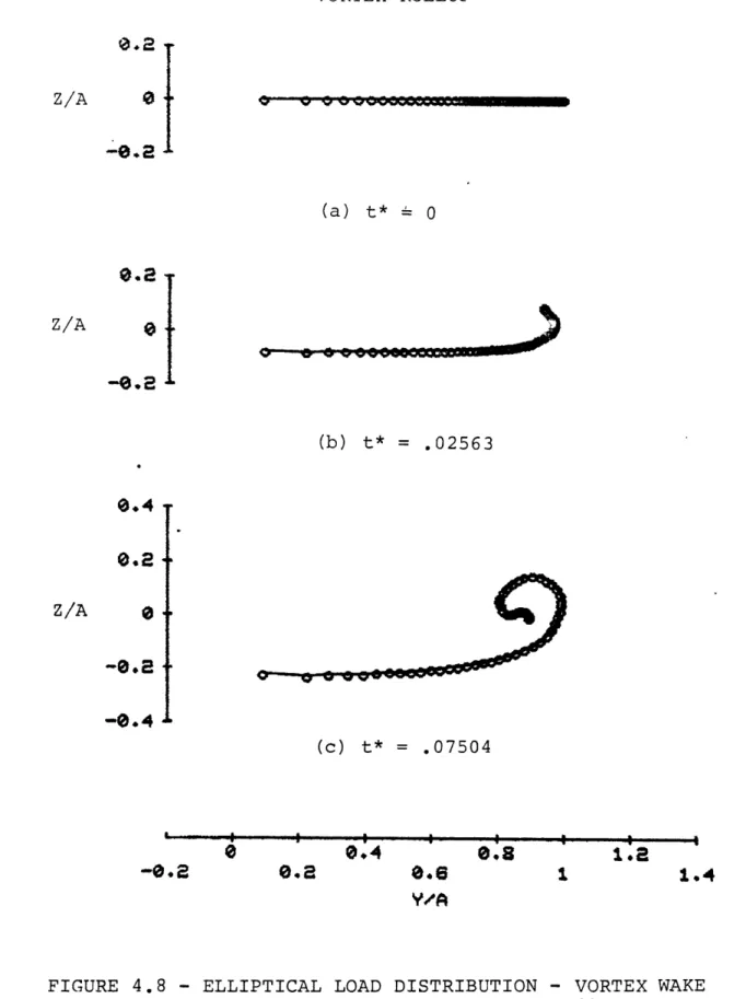
4.8 Elliptical Load Distribution - Vortex Wake 108 Geometry, Constant Strength Point Vortices,

60 Points, Grid = 31x31 4.8a t* = 0 108 4.8b t* = .02563 108 4.8c t* = .07504 108 4.8d t* = .15714 109 4.8e t* = .25539 109 4.8f t* = .36155 110

4.9 Elliptical Load Distribution - V Velocity Profile, 111 Constant Strength Point Vortices, 60 Points,

Grid = 31x31

4.9a t* = 0

.4.9b t* = .36155 112

4.10 Elliptical Load Distribution - W Velocity Profile, 113 Constant Strength Point Vortices, 60 Points,

Grid = 31x31

4.10a t* = 0 113

4.10b t* = .36155 114

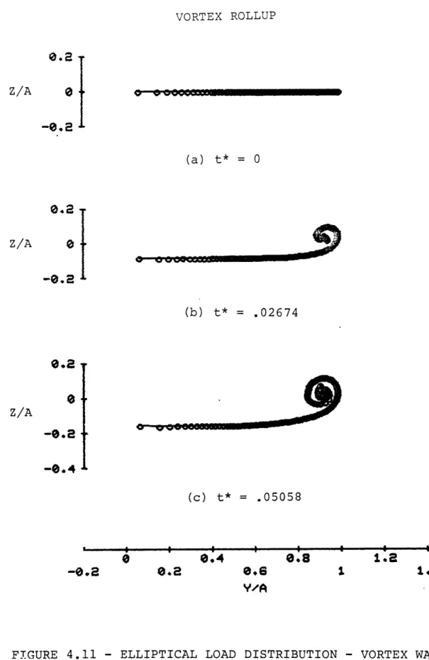
4.11 Elliptical Load Distribution - Vortex Wake 115 Geometry, Constant Strength Point Vortices,

120 Points, Grid = 61x61 4.lla t* = 0 115 4.1lb t* = .02674 115 4.11c t* = .05058 115 4.lld t* = .07680 116 4.lle t* = .10064 116

4.12 Elliptical Load Distribution - V Velocity Profile, 117 Constant Strength Point Vortices, 120 Points,

Grid = 61x61

4.12a t* = 0 117

4.12b t* = .10064 118

4.13 Elliptical Load Distribution - W Velocity Profile, 119 Constant Strength Point Vortices, 120 Points,

Grid = 61x61

4.13a t* = 0 119

4.13b t* = .10064 120

4.14 Elliptical Load Distribution - Spanwise Variation 121 of Vortex Centroid with Time

4.15 Elliptical Load Distribution - Vertical Variation 122 of Vortex Centroid with Time

4.16 Wing Loading and Shed Wake Strength - Simulated 12.3 Flap Loading

4.17 Simulated Flap Loading - Vortex Wake Geometry, 124 Constant Strength Point Vortices, 130 Points,

Grid 31x31 4.17a t* = 0 124 4.17b t* = .02925 124 4.17c t* = .07995 124 4.17d t* = .15266 125 4.17e t* = .20712 125

4.18 Simulated Flap Loading - V Velocity Profile, 126 Constant Strength Point Vortices, 130 Points,

Grid = 31x31

4.18a t* = 0 126

4.18b t* =..20712 127

4.19 Simulated Flap Loading - W Velocity Profile, 128 Constant Strength Point Vortices, 130 Points,

Grid = 31x31

4.19a t* = 0 128

4.19b t* = .20712 129

4.20 Simulated Flap Loading - Vortex Wake Geometry, 130 Equally Spaced Point Vortices, 130 Points,

Grid = 31x31 4.20a t* = 0 130 4.20b t* = .02915 130 4.20c t* = .07976 130 4.20d t* = .15223 131 4.20e t* = .20658 131

4.21 Simulated Flap Loading - V Velocity Profile, 132 Equally Spaced Point Vortices, 130 Points,

Grid = 31x31

4.21a t* = 0 132

4.21b t* = .20658 133

4.22 Simulated Flap Loading - W Velocity Profile, 134 Equally Spaced Point Vortices, 130 Points,

Grid = 31x31

4.22a t* = 0 134

4.22b t* = .20658 135

4.23 Simulated Flap Loading - Vortex Wake Geometry, 136 Constant Strength Point Vortices, 65 Points,

Grid = 31x31 4.23a t* = 0 136 4.23b t* = .02903 136 4.23c t* = .07988 136 4.23d t* = .15276 137 4.23e t* = .20659 137

4.24 Simulated Flap Loading - V Velocity Profile, 138 Constant Strength Point Vortices, 65 Points,

Grid = 31x31

4.24a t* = 0 138

4.24b t* = .20659 139

4.25 Simulated Flap Loading - W Velocity Profile, 140 Constant Strength Point Vortices, 65 Points,

Grid = 31x31 140

4.25a t* = 0 141

4.26 Simulated Flap Loading - Vortex Wake Geometry, 142 Constant Strength Point Vortices, 130 Points,

Grid = 61x61

4.26a t* = 0 142

4.26b t* = .02567 142

4.26c t* = .05206 142

4.26d t* = .07749 143

4.27 Simulated Flap Loading - V Velocity Profile, 144 Constant Strength Point Vortices, 130 Points,

Grid = 61x61

4.27a t* = 0 144

4.27b t* = .07749 145

4.28 Simulated Flap Loading - W Velocity Profile, 146 Constant Strength Point Vortices, 130 Points,

Grid = 61x61

4.28a t* = 0 146

4.28b t* = .07749 147

4.29 Simulated Flap Loading - Spanwise Variation of 148 Vortex Centroids With Time

4.30 Simulated Flap Loading - Vertical Variation of 149 Vortex Centroids With Time

4.31 Wing Loading and Shed Wake Strength - Rotating 150 Wing Loading

4.32 Rotating Wing Load Distribution - Vortex Wake 151 Geometry, Near Wake Represented by Concentrated

Point Vortices, 3 Points on Each Vortex Wake, Grid = 61x81, Relaxation Coefficient = .1

4.32a Wake Iteration = 1 151

4.32b Wake Iteration = 10 152

4.32c Wake Iteration = 20 153

4.32d Wake Iteration = 30 154

4.32e Wake Iteration = 40 155

4.33 Rotating Wing Load Distribution - Vortex Wake 156 Geometry, Near Wake Represented by Many Point

Vortices, 30 Points on Each Vortex Wake, Grid = 61x81, Relaxation Coefficient = .2

4.33a Wake Iteration = 1 156

4.33b Wake Iteration = 5 157

4.33c Wake Iteration = 7 158

4.33d Wake Iteration = 10 159

4.33e Wake Iteration = 13 160

A.l Complex Plane Representation for a Point Vortex 161 A.2 Complex Plane Representation for a Pair of 161

Reflected Vortices

A.3 Jump Conditions Across Singularity Branch Cuts 162 B.1 Schematic for "Cloud in Cell" Redistribution 163

Scheme

C.1 Geometry of Rotating Wing Wake 164

C.2 Far Wake Model 165

C.3 Far Wake Boundary Condition - Integration 166 Techniques Around Computational Boundary

LIST OF SYMBOLS

a,A Semi-span Al

A2 Areas used in "CIC" scheme A3

A4

F(a0 Complex potential

j

N Summation index for point vortices on computational mesh

NF Summation index for the far wake model

NI Summation index for the intermediate wake model

n Integer value, 0, ±l, ±2, R Rotor blade tip radius

t Time

4 t Time increment

v, V Velocity component in y direction w, W Velocity component in z direction W, Initial W velocity

x, X Cartesian coordinate, positive downstream y, Y Cartesian coordinate, positive out right wing

A y Computational mesh spacing in y direction y ,y End points of span increment

y4. Cartesian coordinate of tip vortex centroid z, Z Cartesian coordinate, positive up

&z Computational mesh spacing in z direction

Azn Wake spacing in far wake

bzw Wake spacing

Angle in far wake analysis Blade separation angle (7 Circulation

q.9 Circulation of ith point vortex w. Circulation of lifting surface

Circulation of lifting surface at symmetry plane (y=0)

Position angle from point vortex to flow field Dimensionless velocity,

2

( ) Non-unique value at branch cut ( )* -Dimensionless quantity

( ) Quantity used in complex plane ( ) Value above branch cut

( )~ Value below branch cut o( ) Order of

SECTION 1 INTRODUCTION

1.1 Importance of Non-planar Vortex Wake Analysis

The design and analysis of conventional and rotating wing vehicles are restricted by inadequate means of computing the development of non-planar vortex wakes. The majority of

design codes developed to date utilize a linear wake model to represent the vortex wake generated by a lifting wing. In reality, the vortex wake rolls up into concentrated vortex cores within a short distance downstream of the trailing edge. For an isolated wing and body, the induced velocity

distribution at the wing plane, except perhaps at the wing tip, varies insignificantly due to the redistribution of the vorticity in the rolled up wake. For this reason, the

development of wing-body codes has not been limited

significantly by the linear wake model. Unlike the wing-body configuration, for many configurations, this is strictly not

so. Some important ones are.

1. Empennage: Vortex wakes shed from the wing propagate downstream very near the empennage. For a transport aircraft at cruise condition, the influence of the non-planar vortex wake may not be significant due to the location of the tip vortex core outboard away from the horizontal tail. However, during pitch-up and maneuver, when the wing is highly

loaded, the wake quickly rolls up into concentrated vortex cores which will be much closer to the

empennage. The non-planar vortex wake should be modeled.

2. Canard-Wing: The vortex wake generated by a canard wing will interact directly with the wing flow

field. The non-planar vortex wake should be

modeled to provide accurate loading distributions on the wing.

3. Delta Wings: The flow at the leading edge of a delta wing separates at moderate to high incidence and

develops into a vortex wake above the wing. The non-planar wake model is essential in this

analysis.

4. Helicopter Rotors: Design of rotating wing vehicles is significantly limited by accoustic and'vibration constraints. Blade-vortex wake interaction

contributes the major influence on these constraints. Non-planar vortex wake models are needed to

correctly predict this interaction.

Non-planar vortex wake models will enhance the analysis of many aircraft configurations. For some configurations, non-planar vortex wake models are a necessity. It is

therefore desirable to develop methodologies to treat

non-planar vortex wakes. This report presents such a method for simplified problems and, hopefully, represents the first

step in the development of a method for the above mentioned configurations.

1.2 Previous Investigations

1.2.1 Vortex Flows and Conventional Wings

Analysis of the incompressible, inviscid interaction and propagation of isolated singularities (point vortices) in an otherwise irrotational flow field dates back to the early work of Rosenhead [1] and has received considerable attention in the past ten years. When the fluid is considered ideal, except

for isolated singularities, the theorems of Helmholtz and Kelvin are applicable to a control surface convected with the

flow and encompassing the singularities. In accordance with these theorems, the transport or convection of the vorticity throughout the control surface is determined by the local fluid velocity which, in turn, is induced in the flow field by the point vortices. This approach was utilized by Rosenhead and

formed the foundation for a number of investigations that

followed. In this approach, with knowledge of the location and circulation strengths of the point vortices, the velocity field induced by the point singularities can be calculated by use of the Biot-Savart relation. Since the flow is ideal and the problem is linear, the solution of the flow field for any

number of vortex points may be determined through superimposing the induced velo6ities of the individual singularities. A

point vortex does not induce a velocity on itself. The point vortices are convected by the local flow field velocity. After

which, at a short time interval later, a new induced flow field emerges and the point vortices are convected again. This point tracking or Langrangian method is applied to convect the point vortices while the velocity field is determined by summing the effects of the point vortices.

The work of Rosenhead and, more recently, Moore [2] approximates a vortex wake by a finite number of point vortices or vortex markers and determines the

three-dimensional rollup of the non-planar vortex wake through a two-dimensional time dependent solution. This two-dimensional plane, which is convected with the free stream velocity, is called the Trefftz plane and remains perpendicular to the free stream (see Figure 1.1). The

two-dimensional time dependent solution using the point vortices and the Biot-Savart relation often resulted in

instabilities and chaotic vortex motion. The instabilities stem from the singular nature of the vortex points. In a paper by Chorin et al [3], the nature of the singularities was

investigated. In this paper, it was shown that if the point vortices are smoothed out or given a finite radius, the

instabilities disappear and the vortex rollup is smooth. The previously described full Lagrangian approach has significant inherent computational burdens. In the above method, for N point vortices, a number of operations of order N2 are required to determine the flow field. This condition puts a burden on the number of point vortices used to define

the vortex sheet. Instead of isolating each point vortex, increased computational efficiency can be achieved by grouping a number of the point vortices together. After which, the velocity field is then calculated. This concept leads to the concept of "Vortex in Cell" or "Cloud in Cell" and suggests the Eulerian-Lagrangian approach to the solution.

The Eulerian-Lagrangian approach, coupled with the "Cloud in Cell" technique, has been employed by a number of authors [see for example, [4,5,6]]. The solution to the point vortex convection remains Lagrangian, but the velocity field is determined from the stream function in an Eulerian manner. The stream function is determined on the Eulerian mesh as the solution to Poisson's equation. In this method, the vorticity is redistributed to the mesh nodes using a bilinear interpolation scheme. The Poisson equation for the stream function can now be solved with the vorticity on the right-hand side of the equation. The velocity field is determined from the stream function and then bilinearly interpolated to the point vortices. The point vortices can now be convected. The redistribution scheme or "Cloud in Cell" technique of this method accomplishes a result similar to that of Chorin [3]. The point vortices are smoothed and the instabilities are suppressed.

Baker [4] completed extensive investigations on the rollup of vortex wakes generated by elliptically loaded wings and by wing loadings simulating deflected flap configurations.

Typically, in his investigations, Baker represented the vortex wake by 2,000 point vortices. Instabilities are shown in the tip vortex core and in some portions of the vortex wake in some of the results. Christiansen [5]

demonstrated the utility of the technique through numerous applications.

Three-dimensional calculations of the non-planar vortex rollup problem are, for the most part, determined through the use of panel methods. In general, the analysis is conducted to more fully understand flow characteristics about wings and

wing-body combinations with leading edge vortex separation. Johnson et al [71 used panel methods to model the development of vortex structures shed from the leading edge of delta wings. Here again, the vortex sheet is tracked in a Lagrangian fashion and the influence of' the vortex singularities is included in the calculation of the velocity field. Owing to the

complexity of the three-dimensional problem, the shed vortex wake is parameterized and the vortex wake singularity

strengths are determined as part of the singularity solution. The findings of Johnson [7] indicate that if the real flow deviates significantly from the single vortex structure

predicted by the flow model, the analysis will generally tend to fail.

1.2.2 Rotating Wings

Applications of vortex methods to understand and,

consequently, alleviate the accoustical and vibratory patterns associated with rotary wing vehicles have increased

significantly in the past five years. Extensive surveys of numerical analysis'applied to rotating wings are presented in

[8] and [9] and are highlighted here for completeness. Emphasis on the distorted wake analysis is presented here.

The development of the "semi-rigid" wake concept was initiated by Miller [10] and marked the inception of the

distorted wake analysis. Previously, the undistorted wake was represented by a semi-infinite cylinder emerging from the tips of the rotor blades. This cylindrical model implies an

infinite number of blades and, therefore, will yield no information about the periodic vortex wake known to exist. Accoustical and vibratory analysis is not possible for the

cylindrical wake model, but the "semi-rigid" wake would provide a wake model needed for this analysis.

Several authors [11-13] investigated further the

"semi-rigid" wake concept to represent the structure of the rolled up tip vortex and to estimate the influence of the

vortex on the rotor blade loading. This model has fallen short of representing the real wake. Large discrepancies between the calculated and measured wake geometries have been shown by Ham

[13]. More accurate wake models were needed. Simplified

the wake geometry were developed by Brady and Crimi [14].

Extensions of the vortex ring model and a method to include the rollup of the two concentrated tip vortices was developed by

Levinsky [15].

A more complex method used to calculate the effects of the wake geometry, which is free to distort under the influence of

the flow field, was developed by Landgrebe [16, 17]. For this method, the vortex wake is represented by a finite number of vortex "filaments" which convect and interact under the

influence of the local velocity field. However, in this analysis, the wake is allowed to distort only after the wake has been predescribed. Landgrebe [17] predescribes the wake as being grouped into a strong rolled up tip vortex filament and several weaker filaments representing the inboard portion of the vortex wake. Knowledge of the predescribed location of the vortex filaments is gained from experimental results and will limit the analysis owing to this empiricism. Summa and Clark [18] have represented the blade lifting surface through the use of vortex lattice techniques. The wake is described with techniques reported by Landgrebe.

At present, the work of Miller [19] is the only

investigation devoted to the free wake analysis of rotating wing devices which is not restricted by the empiricisms

associated with the wake geometry. In this analysis, the wake geometry is divided into three sections: the near wake; the

straight semi-infinite vortex filaments extending from the rotor blade trailing edge. Using the Betz [22]

approximation, this wake is rolled up into three concentrated vortices for the three regions of the load distribution as

shown in Figure 1.2. These three vortices, whose initial position is given by the Betz approximation, are used to represent the intermediate wake. For the Betz

approximations, the tip vortex is represented by the wake rollup from the tip to the maximum circulation and a second vortex is represented by the rollup from this maximum to the point where the slope of the loading tends to zero. The root vortex is represented by the remaining portion of the load distribution. The far wake is represented by a semi-infinite vortex cylinder for the three-dimensional analysis and by two semi-infinite vortex wakes for the two-dimensional analysis

(see Figure 1.3).

A new distribution of the intermediate wake is

determined from the induced flow field velocities. Induced flow field velocities at the rotor blade plane are then

calculated from the influence of the near wake, intermediate wake and the far wake. The vortex wake shed from the blade is then recalculated and the cycle repeats. The iterative process continues until the induced velocities at the blade location have reached convergence. In Miller's analysis [19] and in predictions by Betz's theory, the emergence of a

indicate a strong tip vortex, at present, the mid-span vortex has not been measured. The effect of this vortex on the

blade loading at large distances may be small, but when the vortex is in close proximity of the blade, significant errors in the predicted blade loading may appear. Analysis to

verify the existence of the mid-span vortex is needed. This survey is intended to bring to light the current status of rotating wing wake analysis and to motivate the current analysis in order that a better model of the vortex wake may be obtained.

1.3 Current Investigation

The two-dimensional time dependent solution for the rollup of non-planar vortex wakes with use of the existing

Eulerian-Lagrangian method [4, 5] is restricted in that an extension of the analysis to three-dimensions is not

possible. In order to investigate the development of

non-planar vortex wakes in three-dimensions, the flow field must be described by use of the velocity potential rather

than the stream function. While this paper does not deal directly with the three-dimensional problem, the first step in the analysis (two-dimensional time dependent problem for conventional wings or two-dimensional steady state problem for rotating wings) is presented.

1.3.1 Vortex Flows and Conventional Wings

In this section, an introduction is given for the problem solved in the pres.ent investigation. Detailed

development of the theoretical and numerical treatment is given in Sections 2 and 3.

1) Governing Equations, Boundary Conditions, Initial Conditions and Jump Conditions

In order to specify the problem, the governing

equations and boundary conditions must be clearly stated. The calculations of the flow field are performed on the Trefftz plane for an ideal fluid. The vorticity is considered here to be scalar and corresponding to a vorticity vector directed parallel to the free stream. The vorticity vector is a doubly infinite line

vortex. The vortex wake is represented by distributing point vortices along the width of the vortex wake on the Trefftz plane. Everywhere in this investigation, a

vortex wake symmetric about the y=O plane is modeled. Owing to this symmetry, calculations are necessary on the Trefftz Plane for y> only. The influence of the reflected wake is modeled through the boundary

conditions. Laplace's equation for the velocity

potential governs the flow field. Boundary conditions on the velocity potential are determined from the flow field induced by line vortices (see for example,

distributed along a z = constant line and has extent 0±

y 4 1.

In contrast to the flow field solution using the stream function, solutions obtained using the velocity potential will be multivalued. (See for example [201)

In order to retain a unique solution, it is necessary to construct branch cuts extending from the singularities to + 00 and to apply appropriate jump conditions at this cut. To illustrate this condition, consider the figure below.

-Tv-As illustrated in this figure, the jump conditions are needed between the reflected vortices only (the jump conditions cancel identically to the right of the right vortex for a reflected pair of vortices). (Appendix A)

The velocity field is determined from the gradient of the potential and the motion of the point vortices is

calculated from the trajectory equations of motion. These topics are discussed fully in Section 2.1.

2) Singularity Redistribution and Velocity Determination

For the solution of the velocity field on the

Eulerian mesh, the vorticity must be redistributed if it is to be accurately included in the analysis. An

adaptation of the "Cloud in Cell" technique is used to redistribute the vorticity. The vorticity is

redistributed to the centroids of the four nearest mesh cells. See figure below.

A7 4

/7-

174- 41~ # fit

New branch cuts are constructed for each of the newly redistributed points. After the potential field is solved, the velocity at the location of the point vortex markers is determined using bilinear

interpolation from the velocities of the four nearest mesh centroids. Only information from mesh cells

affected during the vorticity redistribution is used in the velocity determination (see Appendix B).

3) Method

Solutions to the non-dimensional forms of the governing equations, the boundary conditions and the initial conditions are determined through the use of finite difference techniques.

Initially, the input vorticity is distributed along the z=O axis. The vorticity is redistributed to the centroids of the mesh cells and the boundary conditions determined from the new distribution of vorticity.

The components of the flow field velocity are set

everywhere to zero at t=O. Laplace's equation for the velocity potential is now replaced by a central

difference equation. Jump conditions for the new

distribution of vorticity are calculated and introduced into the finite difference forms of the Laplace equation and the w velocity equation. The difference equations are solved using successive line.over-relaxation (SLOR) or a direct solver for elliptic partial differential

equations [24]. The flow field velocities are

determined from the gradient of the potential. The

motion of the point vortices are calculated according to the equations of motion, after which, the vorticity is convected and the Trefftz plane is stepped forward

(downstream) in time. The new vortex wake is

redistributed and the cycle repeats. A flow chart is shown in Figure 1.4.

1.3.2 Rotating Wings .

The solution to the non-planar vortex wake flow field for rotating wings is obtained on an Eulerian mesh. Unlike the two-dimensional time dependent problem for conventional wings, we week the steady state solution to the flow field

for the rotating wing problem. By steady state, we mean that the helical rotor wake below the rotor blade is invariant with blade rotation for a given blade loading.

In this analysis, as in the analysis for conventicnal wings, the vortex wake or wakes on the computational plane

are represented by intersections of doubly infinite line vortices with that plane. The time dependent solution for conventional wing analysis (Trefftz plane representation) was obtained by integrating along the vortex trajectories with respect to time. In the steady state solution for rotating wing flow fields, the wake geometry below the rotor blade is obtained by integrating along the helical rotor wake with respect to arc length. Consider a single point vortex illustrated below.

WA--

Al---If the location of A is known, the position of B can be determined by integrating the trajectory equation of motion along the helical path. This will be discussed further in Section 2.1.2.

1) Governing Equations, Boundary Conditions, Initial Conditions and Jump Conditions

Here, again, the flow of an ideal fluid is

field is obtained on a computational plane illustrated in the figure below.

Vortex wakes representing the rotor blade and the

intersections of the helical rotor blade wake with the computational plane are distributed on this plane. The computational plane extends from just above the vortex wake representing the rotor blade to negative infinity

below the rotor blade.

On this plane, three distinct regions representing the helical rotor wake are modeled. The three regions will be termed; the near wake, the intermediate wake and the far wake. See figure below.

The near wake represents the rotor blade and the first four intersections of the helical rotor wake with the computational plane. The computational mesh is constructed on the computational plane and, in general, will encompass the near wake only.

The intermediate wake is represented, initially, by concentrated point vortices of strengths and locations predicted by Betz [22] theory. The intermediate wake

represents the next ten intersections of the helical wake with the computational plane. The far wake is

similar to the intermediate wake, but extends to -00. The intermediate wake will generally be outside the computational mesh and the far wake will always lie outside the mesh. Boundary conditions for the near and intermediate wakes are calculated in the usual way and represent the influence of line vortices. The influence of the far wake on the boundary conditions is modeled using an asymptotic expansion over the length of the far wake. See Figures 1.5 and 1.6. Further development of the intermediate and far wake models can be found in Appendix C.

Initially, the input vorticity on the computational mesh will be distributed along lines of constant z or

axial distance. These distributions represent the near wake. The spacing of this tiered structure (see Figure

rotor. Miller [19] determined that the solution was not sensitive to the number of input wakes beyond a minimum of four plus the blade representation. The flow field velocities and the potential are set similarly to values

described before. These topics are discussed further in Section 2.1.

2) Singularity Redistribution and Velocity Determination The singularity redistribution technique and methods for determining the velocities of the point vortices are directly extended to N vortices and are exactly those described in the previous section (also see Appendix B). 3) Method

A) Initially, the vorticity is input in the

previously described tier structure and represents the shed wake for the rotor blade loading. The vorticity in the wake is represented by point vortices at the intersection points of the doubly

infinite line vortices with the computational plane. The first or uppermost (z=0) wake

represents the blade. This first wake or blade wake is considered fixed on the computational mesh

and does not rollup, but retains the signature of the blade loading.

B) The vorticity is redistributed and the

boundary conditions calculated from the influence of this and the intermediate and far wake

vorticity. Jump conditions are calculated in the usual way (Appendix A). Laplace's equation for the velocity potential is again solved using SLOR or a

direct method [24] and the velocity field calculated from the potential.

C) The induced velocities at the blade location, z=O, are calculated and examined for convergence. If the velocities have converged, the steady state rotor wake flow field is known. If the induced velocities have not converged, a new distribution of vorticity is calculated and control returns to B. The new distribution of vorticity in the near wake below Ehe rotor blade is determined by

integrating along the helical vortex trajectories from the fixed rotor blade location to each vortex wake. For a two-bladed rotor, the first wake below the rotor blade would be obtained by integrating

from 0 to 77, the second wake by integrating from 0 to Z17 and so forth. A flow chart is shown in

SECTION 2

FORMULATION OF PROBLEM

The two-dimensional flow field for an incompressible, inviscid and irrotational (except for isolated vortex

singularities) fluid can be represented by a potential

function 9 . Here is the velocity potential and, for the fluid described above, satisfies Laplace's equation

everywhere in the defined flow field. The velocity in the flow field can be calculated directly as the gradient of the potential.

When the problem is solved on a two-dimensional plane, such as the Trefftz plane, the problem is thought of as a

boundary value problem. The boundary conditions are determined uniquely from the vorticity distributed on the plane. The

continuous distribution of vorticity on the plane is often represented by a finite number of point (line) vortices. This representation creates a singularity problem which was not present in the continuous definition of the vorticity. The point vortices are branch points and branch cuts must be extended from each singularity. Jump conditions are applied across the cuts in order that the solution remain unique.

This section will present the development of the governing equations, dimensionless forms of the equations and

2.1.1 Conventional Wings

For the two-dimensional, incompressible, inviscid fluid flow under consideration, the governing equation can be

described by the Eulerian equations:

V O (2.1)

-~ c (2.2 a, b)

together with the boundary condition:

(2.3)

where I is the circulation of the ith point vortex and $. is the angle from the positive y axis to the boundary point. (See Figure 2.1) Here, the summation over N represents the

contributions of the point vortices on the computational plane and the corresponding reflected image vortices.

The initial conditions for the vortex wake are

determined from the wing loading or circulation, / (y). If we consider the wake vorticity to be given by

P

for the continuous (non-discretized) problem, the initial wake vorticity is given by:

Id

For the numerical problem, this continuous vorticity distribution is lumped into discrete vortex markers, each designated by the index i where i=1,N and N is the number of markers. The strength of each marker is:

S()--(2.4)

where = circulation of ith vortex in wake = load distribution on lifting surface = limits on span increment defining = position of ith vortex y

The solution to equations 2.1-2.4 is termed the Eulerian problem. Instead of solving for the transport of vorticity on the Eulerian mesh, a discrete point or Lagrangian method is utilized. In the Lagrangian method, the trajectory

equations of motion are solved to determine the convection of the point vortices. They have the form:

V(J~f) WIy~ij (2.5a,

b)

where yg, zg are the coordinates representing the ith point vortex location. The solution to equations 2.1-2.5 is termed the Eulerian-Lagrangian method and is the foundation

2.1.2 Potatineq Wings

The solution to vortex wakes of rotating wings is calculated on a computational plane (Figure 1.5) and is governed by equations 2.1 and 2.2. The time dependent trajectory equations of equation 2.5 are not applicable to the steady state solution for rotating wing flow fields. The trajectory equations used in this steady state solution are defined later in this subsection. The boundary conditions and initial conditions differ from those for conventional wings.

For rotating wings in the hover condition, a helical vortex wake structure extends. from the rotor disk to z= -00 . The wake near the rotor disk is represented by individual vortex wakes, each composed of many vortex markers. The

remainder of the wake is approximated by the semi-infinite vortex wake model (see Figure 1.6). The boundary condition

for the potential on the computational domain is calculated by superimposing the effects of the individual wakes and the semi-infinite vortex wake. The vortex wakes on the

computational mesh are represented by point vortices which have the boundary condition of equation 2.3. The boundary condition for the intermediate vortex wake has the form:

Z

r

7(2.6)

where NI is the total number of point vortices in the

intermediate wake and the corresponding reflected image vortices.

The boundary condition for the far wake is developed in Appendix C and is given by equation C.9.

As with the conventional wing, the rotor loading

distribution is discretized to give the strength of the wake vortex markers. However, markers must be initially placed not only at the rotor trailing edge, but also in wakes spaced apart below the rotor.

The initial vortex wake definition on the computational mesh is then:

J=

r1 )(2.7)

where the notation is that following equation 2.4 and At is determined from the flow through the rotor.

Miller [19] has determined that the solution is

insensitive to the number of input wakes beyond a minimum of four. In this analysis, four input wakes plus the blade representation are modeled.

The trajectory equations of motion are now spatially dependent rather than time dependent as was shown in equation 2.5. Here, the trajectory equations of motion define the helical trajectory of each vortex marker in the near wake definition. The spatially dependent trajectory equations of motion are obtained from equation 2.5 as follows:

Yet W

~

ddt

where dt represents the time for the next rotor blade passage.

Then:

y(

YA"L

Where

X

7

The trajectory equations become:

2.1.3 Betz Approximations

Theoretical methods to determine the location of fully rolled up vortex structures generated by lifting wings were derived by Betz [22] and elaborated on by Donaldson [23]. The theory relates the loading on the wing to the fully developed vortex structure by utilizing three conservation laws. The conservation laws satisfied are: conservation of circulation; invariant spanwise centroid of vorticity; and conservation of the second moment of vorticity. Development of the theory is outlined in Donaldson [23] and the results are shown here for convenience.

Consider the load distribution shown in Figure 2.2. The load distribution will generate three separate vortex cores. We assume that all the vorticity shed outboard of point A will roll up into the tip vortex, that the vorticity between points A and B will roll up into the mid-span or flap vortex and all vorticity between B and the aircraft symmetry plane, y=O, will roll up into the inboard vortex.

The centroid of the rolled up vorticity for region A-B is defined by:

w e i s t e co

9

The total circulation of the vortex is equal to:

178A

d%

(2.10)

These results will be used later to compare the centroids of vorticity with those predicted by the current investigation.

2.2 Dimensionless Forms of the Equations

The dimensionless forms of the governing equations are developed in this section. The non-dimensionalization of the conventional wing and rotating wing problems are slightly different, corresponding to the different notations used in the respective literatures.

2.2.1 Conventional Wings

Dimensionless forms of the equations of Section 2.1 may be obtained by introducing the following dimensionless

parameters:

(2.11)

T-where,

a

= circulation at wing root section

Wo = initial downwash at the semi-span location due to a vortex of strength L at y=0.

Using the conventions of equation 2.11, the governing equations take the form:

z 0(2.12)

J

On the boundary,

(2.14)

where N is the sum over the point vortices and the

corresponding reflected images. The trajectory equations for the vortex markers become:

A~i:v%~/),

q4..

W&

*)

(2.15)

Equations 2.12 and 2.13b will have different forms at the branch cuts. See equations A.16 and A.17, Appendix A.

2.2.2 Rotating Wings

Dimensionless forms of the equations of Section 2.1 can be obtained by introducing the following dimensionless parameters:

j -

(Z

-

O

JU

W--s

= rotary disk radius

y 4 e

= angular velocity

tA)O = tip speed.

With the convention of equation 2.16, the governing equations become:

C

LAJ~e)0'

*K.

xf/WO

it

//.I,.

z

*

)o 41C

On the boundary for the near and intermediate wakes.

/

ZT17

z

g*~.

where N+NI is the sum over the point vortices and the

corresponding reflected images in the near and intermediate wakes.

On the boundary for the far wake.

- a - d 9

A_

3eL

(2.20)

Here, the summation represents the summation over the three point vortices defining the far wake and a, b, c are given in

equation C.10.

The trajectory equations of motion become:

t-

'

_A

_-1

(2.21)

The variation by a constant between the dimensionless forms of the governing equations for conventional and

rotating wings results from the dimensionless conventions for each configuration.

The description of the dimensionless forms of equations 2.17 and 2.18b at the singularity branch cut will be

discussed in Section 2.3 and later in Section 3.1. See equations A.18 and A.19, Appendix A.

2.3 Single Value Restrictions on the Velocity Potential The distributed point vortices representing the vortex wake are branch point singularities. When the flow field is described by use of the velocity potential, the solution will be non-unique unless restrictions on the potential are imposed. After each full cycle around a vortex singularity, the

potential will either be increased or decreased by the strength of the vortex singularity (the sign of the change depends on the direction of the path and the direction of the circulatory flow). For the potential to remain single valued, jump

conditions are included in the analysis to compensate for this change in the potential. A summary of these conditions follows. Full details are presented in Appendix A.

The complex potential generated by a point vortex at z=O can be written:

-

/~,(2.22)

~

where /' is strength of the circulatory flow, the "flow is counterclockwise for

gO.

The extension of equation 2.22 to a pair of vortices of equal and opposite strengths with positions 2 = a is

represented by:

A< )Z

(2.23)

then

2/fTp

-

I7E/)

Z7=

1

f /

where +70-are position angles from z '=t.to point z' and m,n are integer values.

It follows from equation 2.23 that the velocity

potential will be an infinitely many valued function. In order to investigate this further, we construct branch cuts

from each point vortex to + cO along the real axis. Then, if a simple closed contour is constructed around each point vortex and the closed contour is traversed in the

counterclockwise direction starting at the branch cut, the following is found (see figure below).

4-~

As the traverse approaches 2 7T (m=l, n=l), the velocity

potential is decreased by on the segment -a y 0 due to the left vortex and increased on the segment a S y f-v due to the right vortex. Then, -the sum of these effects cancel on a 1 y S +*0 and are due to the left vortex only on -a C y a. In order that the velocity potential remains single

valued, the jump condition, o-- -~ ,9= must be

applied on the section -a y 5 a.

SECTION 3

NUMERICAL SCHEME

Solutions to the non-planar vortex wake flow fields are obtained from the solutions of finite difference

approximations for the governing equations. In this

section, finite difference forms of the governing equations, method of solution and accuracy of the method will be

discussed.

3.1 Finite Difference Forms

Finite difference forms of the governing equations are evaluated on an Eulerian mesh. The mesh is to be

rectangular and have constant incremental spacing along the y and z axes (i.e., A y=constant, &z=constant). The analysis considers the vortex wake solutions to wings of span Z4 and evaluates one half of the wake with the influence of the' mirror image wake included in the boundary conditions.

3.1.1 Governing Equations

To obtain the velocity potential, a five-point

centered difference approximation is made to equation 2.1. The equation is generally Laplace in form due to localized vorticity. However, at the singularity branch cuts, the equation has a Poisson form due to the jump conditions. Equation 2.1 has the forms:

7Z#A~J i'-e~i,~k.

fi-2~k.1g4-L-

649-z

ffg..I

Ft

wherer is the dimensionless

rei

ktib

redistributed vorticity. The the figure below.

/ 14 circulation of the lifferencing is illustrated on _ _ _ _ _ _ _ _ _ _ _ _ __

, AAo

A-/

Ji-/

JJ/

Equations 3.1 and 3.2 are dimensionless forms of

equation 2.1 and represent the flow field equations off and on the branch cuts for non-rotating wings.

For rotatinq wing flow fields, equation 3.1 is applied off the branch cut and the form near the branch cut is now:

7 (3.3)

The variation in the right-hand side of equations 3.2 and 3.3 originates from the dimensionless conventions of equations 2.11 and 2.16.

The v and w components of the velocity at the mesh nodes are determined using central difference approximations to the gradient of the velocity potential. This central difference is taken over two mesh cells. The calculation of the v

component of velocity will be indifferent to the existence of the branch cuts. However, jump conditions must be applied at the' cut when central differences of the velocity potential with respect to z are calculated.

The difference equations for the flow field velocities have the forms:

For conventional wings:

- (3.4)

(3.5)

At the branch cut, 3.5 becomes:

~j;k+1

~

wj.: r,, (3.6)

For rotating wing flow fields, equations 3.4 and 3.5 are unchanged and equation 3.6 has the form:

* 94 A-/ &

~-k

Development of the dimensionless forms of the equations appropriate at the branch cut may be found in Appendix A.

The convection of the vortex markers throughout the flow field is calculated from the trajectory equations of motion 2.15 and 2.21. The expressions are different for

conventional and rotating wing flow fields and will be discussed separately.

Equation 2.15 may be written:

dy (3.8)

(3.7)

-L 2t

Equation 3.8 is then integrated over a small time

interval with the velocity held constant for this interval. If the initial time is represented by n and the final time by n+1, then:

!Ii

74

vi9iI

4~

w*h&J&~')

where v-*, w.* are the velocities point vortex

(3.9b)

at the location of the

and g4 < MAX -I/V k

This forward Euler time integration scheme used by Baker has been adopted without investigating further any other schemes.

V -VA Ir-f

Equation 2.21 may be written:

dg

-

VX(3.10)

where I is the blade separation angle in radians. A similar expression holds for z.

If equation 3.10 is integrated along the helical wake over the blade separation angle, the following is found:

-+ 0(3.11)

where is considered constant and equal to the average velocity between k and k+1,

V Wk4. Vi k-4- 4 V .\ /

The velocity of the point vortex is calculated from information at only the nodes of mesh cells affected by the redistribution of the point vortex. This is discussed

further in Sections 3.2 and 3.3.

Boundary conditions on the velocity potential are calculated from the redistributed vorticity on the

computational mesh, plus, for rotating wing analysis, the influence of the semi-infinite vortex wake represented by the intermediate and far wake models. Baker [4] approximated the boundary condition by lumping together neighboring point

vortices into local centroids and then calculating the boundary condition using these centroids. This technique will greatly reduce the computation time. However, in the present

investigation, the boundary condition is calculated exactly from the redistributed circulation in order to evaluate the method.

The influence of the redistributed vorticity on the

boundary values of the potential is related to equations 2.14 and 2.19 for conventional and rotating wing flow fields,

respectively. The potential on the boundary is calculated from the summed influence of the redistributed point (line) vortices. The effect of the semi-infinite vortex wake is represented by equations 2.19 and 2.20 or C.1 and C.10. 3.2 "Cloud in Cell" (CIC) Redistribution Scheme

In order to solve equations 3.1 and 3.3 with the appropriate jump conditions across the branch cuts, the point vortices representing the vortex wake must be

redistributed on the computational mesh. A modified version of the method known as "CIC" is utilized to redistribute the circulation of the point vortices.

In order to accurately model the branch cuts throughout the computational mesh, the circulation of each point vortex is redistributed to the centroid of the four nearest mesh cells, rather than to the nearest mesh nodes [4, 5]. It would be equally accurate to redistribute the circulation to

the mesh nodes, but the redistribution of circulation to the nearest mesh cell centroids was chosen in order to model the branch cut at equal distances from mesh nodes above and below

the four centroids and determines the amount of-circulation to be applied at each centroid. Circulation is conserved within a contour surrounding the four centroids.

The velocity at the point vortex is obtained in the

reverse of the circulation redistribution. See figure below.

344

/ Z

The velocity at the point vortex location is calculated from information at only the nodes of mesh cells affected by the redistribution of circulation. Because the circulation was redistributed to the centroids of mesh cells, it is important to first calculate the velocity at these centroids. The

velocity at the centroid can then be bilinearly interpolated to the point vortex location.

The velocities at the center of each mesh cell edge are calculated using central differences approximations of

equation 2.2a, b over one mesh cell. The velocities at the centroids are taken to be the averages of the values at

opposing mesh edges. The centroid values are then bilinearly interpolated to the'point vortex location. See Appendix B.

3.3 Numerical Solution

This subsecti-on describes the methods and numerical schemes used to solve the finite difference forms of the governing equations. Flow charts describing the method of

solution for conventional and rotating wing flow fields are shown in Figures 1.4 and 1.8, respectively.

Clarification between the methods for conventional wings and rotating wings is presented when appropriate. The method is summarized as follows:

1) Consider an array of N point vortices located at coordinates (yg, zg) and distributed on the

computational mesh; the strength of each vortex being

f1

a lifting surface.. This strength is given by equation 2.4 or 2.7. The point vorticity is

initially along lines of constant z and distributed along this line in one of two ways: a) the vortex wake is represented by equally spaced point

vortices with varying strength; or b) a distribution of constant vortex strength (

constant) and unequal spacing is used. In either case, the contour integral around the shed wake remains constant. For conventional wing analysis, a single vortex wake is input at z=O, 0 t y 5 a.

In the analysis of rotating wings, a minimum of four vortex wakes is input, excluding the blade

representation. Again, each wake is located on a line of constant z, with the wake spacing (in z) determined from the flow through the rotor

(momentum theory). For no variation in the

velocity across the wake, momentum theory provides:

7

(3.12)

where (i = and is the thrust

coefficient. See Figure 1.7. For both analyses, the reflected vortex wake images (-a i y 5 0) are excluded from the computational mesh and included in the analysis mathematically. The point

vorticity contained in the vortex wake representation is redistributed next.

2) The point vortex or circulation redistribution scheme is obtained from a modified version of the "Cloud in Cell" technique. Due to the singularity branch cuts, the circulation is redistributed to the mesh centroids, rather than the mesh nodes (as in [4]). The jump conditions of the redistributed circulation are represented by the right-hand side of equations A.16-A.19. See Appendix A. The influence of the redistributed vorticity on the value of the velocity potential at the boundary can then be calculated.