HAL Id: hal-01840016
https://hal.inria.fr/hal-01840016
Submitted on 16 Jul 2018
HAL is a multi-disciplinary open access
archive for the deposit and dissemination of
sci-entific research documents, whether they are
pub-lished or not. The documents may come from
teaching and research institutions in France or
abroad, or from public or private research centers.
L’archive ouverte pluridisciplinaire HAL, est
destinée au dépôt et à la diffusion de documents
scientifiques de niveau recherche, publiés ou non,
émanant des établissements d’enseignement et de
recherche français ou étrangers, des laboratoires
publics ou privés.
A Salience Measure for 3D Shape Decomposition and
Sub-parts Classification
Thibault Blanc-Beyne, Géraldine Morin, Kathryn Leonard, Stefanie
Hahmann, Axel Carlier
To cite this version:
Thibault Blanc-Beyne, Géraldine Morin, Kathryn Leonard, Stefanie Hahmann, Axel Carlier. A
Salience Measure for 3D Shape Decomposition and Sub-parts Classification. Graphical Models,
Else-vier, 2018, 99, pp.22-30. �10.1016/j.gmod.2018.07.003�. �hal-01840016�
A Salience Measure
for 3D Shape Decomposition and Sub-parts Classification
Thibault Blanc-Beynea, G´eraldine Morina, Kathryn Leonardb, Stefanie Hahmannc, Axel Carliera
aIRIT - Toulouse Institute of Computer Science Research bOccidental College
cUniv. Grenoble Alpes, CNRS (LJK), INRIA, Grenoble INP
Abstract
This paper introduces a measure of significance on a curve skeleton of a 3D piecewise linear shape mesh, allowing the computation of both the shape’s parts and their saliency. We begin by reformulating three existing pruning measures into a non-linear PCA along the skeleton. From this PCA, we then derive a volume-based salience measure, the 3D WEDF, that determines the relative importance to the global shape of the shape part associated to a point of the skeleton. First, we provide robust algorithms for computing the 3D WEDF on a curve skeleton, independent on the number of skeleton branches. Then, we cluster the WEDF values to partition the curve skeleton, and coherently map the decomposition to the associated surface mesh. Thus, we develop an unsupervised hierarchical decomposition of the mesh faces into visually meaningful shape regions that are ordered according to their degree of perceptual salience. The shape analysis tools introduced in this paper are important for many applications including shape comparison, editing, and compression.
Keywords: shape analysis, part hierarchy, medial axis, WEDF, salience measure, 3D shape decomposition
1. Introduction a decomposition of the shape), or similarity detection in a 3D shape, as required by [4].
A key observation is the fact that, despite a repu-tation for instability, a skeleton can provide a reliable basis for shape analysis when it is complemented with measures defined along it. Below, we introduce such a measure, called Weighted Extended Distance Func-tion (WEDF), which is defined on a curve skeleton cen-tered within a 3D shape. WEDF has been introduced re-cently for 2D shape contours [5] and successfully used for defining a salience measure and decomposition of 2D curves [6]. Generalizing to the 3D setting takes two steps: first defining WEDF on a 3D skeleton and deducing a partition, second, mapping the measure on the surface mesh. The second step assesses salience of surface mesh parts: it establishes an injective mapping between surface mesh vertices and the skeleton points while ensuring simultaneously that the inverse mapping produces coherent shape parts. In 2D, a straightforward association of boundary points to the WEDF values of the corresponding skeletal points generates a good par-tition of a shape [6], but the 3D setting is more chal-lenging: a direct extension of the 2D approach to 3D generates a poor partition (see Figure 10, where the Many 3D applications make use of 3D shape
decom-positions in various forms, whether for shape compar-ison and compression, for editing purposes, or for ani-mation. While much work has studied how to produce meaningful parts, there has been little focus on provid-ing additional information on parts, such as their relative importance. In [1], the authors show that decomposi-tion into a hierarchy of part and subparts is memorized by user, and such structure is relevant for shape recogni-tion. Such a measure has been formalized by Hoffman and Singh [2] and called salience of parts. This measure reveals how important a part is to understand the shape as a whole. In this paper, we propose a shape decom-position method that naturally provides insights about parts salience.
The present work makes a first step towards auto-matic similarity-based shape decomposition by intro-ducing a new salience measure for 3D shape decom-position and subparts classification. In particular, the proposed decomposition provides an automatic pre-processing for applications such as structuring a 3D shape (e.g. like [3] whose semantic descriptors relies on
legs run into the body of the ant). Accordingly, we propose a robust algorithm for appropriately transfer-ring the salience measure on the skeleton to the surface mesh, enabling a decomposition into a consistent set of subparts that can be clustered according to their salience levels.
Given a WEDF measure coherently transferred to a surface mesh, we use unsupervised methods for de-composing a 3D shape into subparts and for classify-ing those parts accordclassify-ing to their visual salience. This allows us to determine a primary supporting shape and features with decreasing saliency. In contrast to classical shape segmentation algorithms, our method provides a graded salience-based parts decomposition, where each part is labeled with a value characterizing its importance to the overall shape. Figure 1 shows an example: our method not only segments the body parts from the body, but additionally labels each body part with an importance value so that parts with the same importance value belong to the same level in the impor-tance hierarchy. All rose mesh parts belong to the main body, all green parts to the lowest hierarchy level, all yellow parts to a parent hierarchy level, and so on.
Our hierarchy labels inherit the following two fea-tures from the relationship to the curve skeleton:
• the connectivity of sub-parts including a parent-child relationship starting from the main shape and decreasing monotonically along parts moving away from the main shape is provided, and • the partition and salience measure is stable
un-der volume preserving shape deformation (with no topology change).
Both features allow for a straightforward classification of the extracted sub-shapes into visual salience clusters, which then aids any subsequent computations such as correspondences or local symmetries (see Figure 14).
After presenting related work and giving background in Section 2, we define WEDF on 1D skeletons em-bedded in 3D shapes in Section 4, describe its use for skeletal decomposition in Section 5, and introduce the mapping of the WEDF to the surrounding 3D mesh in Section 6. We then demonstrate the applications of the method for 3D shape decomposition and salience-based evaluation of sub-parts.
2. Related work 2.1. 3D shape salience
Salience, or saliency, is a concept that has been widely studied in the literature. Borji and Itti, in their
important state-of-the-art review [7] define saliency as a characterization of parts of a scene – which could be objects or regions – that appear to an observer to stand out relative to their neighboring parts. Most of the algo-rithms that characterize saliency in images use bottom-up approaches, determining what stands out using low-level cues such as color contrast [8].
A similar approach has been adopted in studies of 3D objects saliency. In their pioneer work, Lee et al. [9] define a mesh saliency measure based on local surface curvature at multiple scales. Many more methods have then be devised following this local approach. Song et al. [10] exploit the apparent correlation between the log-spectrum of 3D mesh geometric Laplacian. They later extended their work, introducing a pooling scheme to introduce a more global saliency [11]. Nouri et al. com-pute local descriptors on each vertex and then a mea-sure of saliency based on a weighted average at di ffer-ent scales [12]. These methods usually compare their results with outcome of user studies, that either cap-tured eye fixations of users watching 3d objects [13], or matched manually designated interest points [14].
In our work, we do not aim at computing a local mea-sure of saliency that would characterize the shape at the vertex level, but rather try to define the relative impor-tance of parts of the shape relative to the whole, thus following Hoffman and Singh’s footsteps [2]. These au-thors emphasize the need for a measure of the salience of visual parts, especially in the context of object recog-nition. A part salience is, according to the authors, cor-related to how much recognizing this part helps recog-nizing the object. The authors propose three features to compute parts salience: relative size of the part, degree of protrusion and boundary strength. As a consequence, for the matter of shape understanding, it is important to be able to discriminate a shape into parts and get a sense of the relative importance of those parts. This is a natural outcome of the work we propose in this paper.
2.2. 3D shape decomposition
3D shape segmentation, or decomposing a shape in sub-parts, is an important research topic offering a wide range of methods emerging from its numerous applica-tions such as compression, reverse engineering, editing, and comparison (see [15] for a recent survey). Super-vised methods are based on user-segmented data and learning methods, offering a perceptually coherent seg-mentation as in [16] or [17]. Unsupervised methods make use of other tools, such as clustering methods or region-growing based on various shape characteristics (e.g. [18, 19], or see [15] for a comparison), spectral
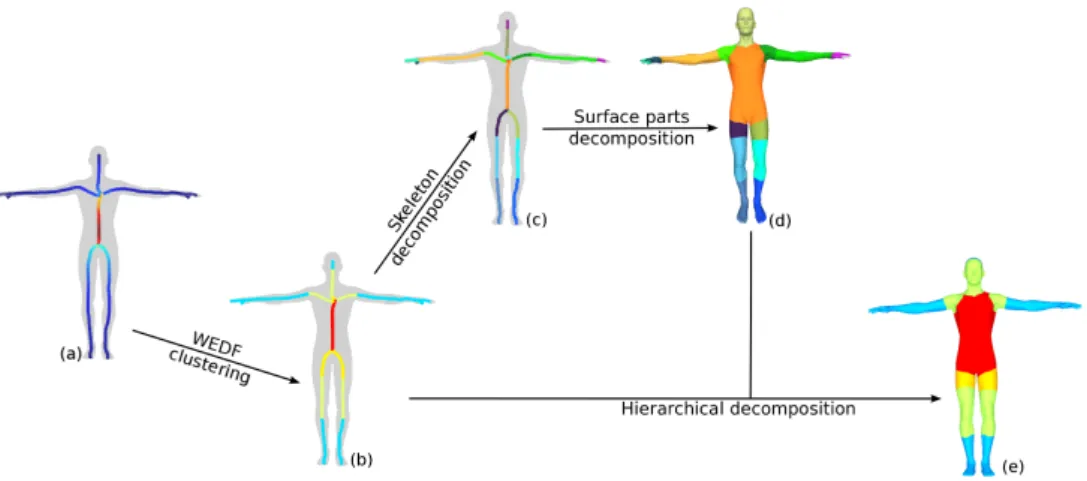
Figure 1: Pipeline of our hierarchical decomposition. Starting from a 3D shape and its curve skeleton, we compute a new measure called WEDF on the curve skeleton(a)and, by clustering WEDF values, we decompose the skeleton into hierarchical parts(b). To each connected part on the skeleton –shown with a different color(c)– a connected region of the surface mesh is assigned(d). Then, a salience value according to the hierarchy is assigned to each corresponding surface part(e)–parts of same importance get a similar color.
analysis (e.g. [20]), spatial subdivision methods or ex-plicit boundary extraction (e.g. [13, 21]), or probabilis-tic models [22, 23]. Other segmentation methods are based on topological information, like Reeb graphs [24] but depend on the function chosen for defining the graph [25]. Skeletons have been applied for segmentation on point clouds, where either the resulting skeletons are not connected [26, 27] or do not provide a consistent segmentation [28], and on surface meshes [29], using the skeleton to define a dense set of possible segmen-tation cuts from which a subset will be chosen based on boundary geometry [30]. Very few of these segmen-tation methods explicitly profit from the innate parent-child relation between sub-parts, or measure for the rel-ative saliency over the parts they obtain.
While most of the 3D methods described above do not make use of skeletons, in part because of their per-ceived instability and difficult to compute, recent meth-ods for 2D shape analysis, decomposition and cluster-ing [31, 5, 6] successfully exploit the geometry of the Blum medial axis for various shape tasks. These meth-ods have shown that the use of the skeletons can be com-plemented with properly chosen functions that provide robustness and stability. One example of such a function is EDF [31] (Extended Distance Function) on 2D shapes which is a useful measure for pruning and has already been generalized to 3D, enabling improved 3D skele-ton computations [32]. Another example is WEDF [5] (Weighted Extended Distance Function), which defines a measure for 2D sub-parts saliency. It has recently been validated through perceptual studies about cogni-tively meaningful shape importance [33] and used for
2D shape decomposition and similarity detection [6]. Our work builds on these 2D structures. We general-ize WEDF to curve-skeletons on the medial axis of a 3D shape, develop an efficient algorithm and provide a per-ceptually consistent, graded salience-based shape de-composition based on the variation of the WEDF along the curve-skeleton (see Figure 2).
(a) (b)
(c) (d)
max
0 Figure 2: Shape center. 3D EDF(a)and 3D WEDF(b) and their as-sociated decomposition (c,d) on a 3D shape.The maximum WEDF value (b,red dot) is centered inside the handle, while the maximum EDF value lies in the tail(a). Our decomposition of the shape into hierarchical salience levels based on each of the two measures given in second row, highlights the fact that considering length, like EDF (c), for measuring salience does not align with perception, whereas considering salience based on WEDF does(d).
2.3. Depth functions in 3D
In 3D, the medial axis of a surface, which consists of the loci of centers of all enclosed maximal balls of the surface, is no longer simply a curve skeleton but gener-ically includes two-dimensional components called me-dial surfaces that intersect transversally creating non-manifold regions. Each point on the medial axis is still
associated to a radius function whose value is the short-est distance to the shape boundary, namely the radius of the corresponding medial ball. A direct extension to 3D of a depth function like EDF is not obvious as there is no single medial axis endpoint associated to a medial component. For this reason, it is more convenient to de-fine functions on some kind of medial skeleton rather than on the full medial axis. Dey and Sun [34] are the first to introduce a mathematical definition and an algo-rithm to compute a medial curve skeleton based on sin-gularities of a so-called medial geodesic function. Yan et al. [32] propose another definition and algorithm of a medial curve skeleton for 3D, based on ET and a burn-ing process over the medial axis. They generalize their work in 2D to define the following functions for 3D on piecewise linear medial axes such as those generated by discrete surface meshes: medial burn time (MBT), ero-sion thickness(ET) and curve burn time (CBT).
In [32], these functions are meant to aid in pruning the medial axis to obtain a simpler version that is more useful in applications, and to obtain a 1D skeletal shape representation. In contrast, our paper aims to provide a new function on the skeleton, similar to WEDF in 2D, able to measure part saliency. To this end, we build on MBT and CBT and derive an efficient algorithm not only for calculating a 3D WEDF along the skeleton but also for returning the function back to the surface mesh in order to determine a salience-based shape decompo-sition and to structure the shape hierarchically.
3. Local analysis of the shape around the axis Before presenting our algorithms in Section 4, let us briefly recall the existing depth functions relevant for our work and introduce an original interpretation of these three measures as a non-linear PCA.
The first two functions are defined on the full medial axis, and are used to extract a curve skeleton. The third is then defined on the extracted skeleton.
• The medial burn time (MBT) is defined as the geodesic distance of a medial axis point to the shape boundary associated to the closest extrem-ity of the widest medial axis sheet containing this point [32].
• The erosion thickness ET is defined as the di ffer-ence between the width and the height: at a point x in a medial axis M, ET (x)= MBT(x) − R(x). ET is used in [32] to determine the scale at which to extract the curve skeleton.
• The curve burn time (CBT) is defined only for skeletal points, and measures the distance to the closest extremity of the shape on the longest skele-ton curve containing the given medial skeleskele-ton curve point. CBT thus corresponds to a length computation, and models the direction in which the shape extends the most. Yan et al.[32] use CBT as a way to prune the medial skeleton to obtain a sim-plified version.
While these measures were intended for simplifica-tion of the medial axis, we show that they can be used as a powerful tool for shape understanding. In partic-ular, the three functions R(x), MBT (x), CBT (x) along a curve skeleton (Fig. 5), when taken together with the paths through the medial axis whose lengths they rep-resent, provide a non-linear version of a PCA decom-position of the shape: at a point x on the curve skele-ton, CBT gives length, MBT gives width and R gives height, and the accompanying curves give the principal directions through the shape starting at x. Note that, un-like in PCA, the directions considered are not linear but follow the curvature of the medial axis along each im-portant direction. Moreover, integrating these quantities (width and height) over the principal direction provides our volume-based saliency measure, the 3D WEDF as introduced in the next section.
4. 3D Weighted Extended Distance Function We now develop a definition for the weighted ex-tended distance function (WEDF) in 3D for piecewise-linear medial surfaces.
The customary challenge in working with discrete medial surfaces is that, in practice, the connectivity of a discrete 3D medial axis is often not consistent with the theory, as noise in the surface mesh propagates to the medial axis sheet by generating regions where the connectivity is rarely manifold even when the underly-ing continuous model would be smooth. This prevents finding a direct, continuous path to the boundary on a medial axis sheet generated from a surface mesh. Such a path is however essential to define a partial order on the medial axis points. The next section introduces the tools necessary to overcome this difficulty.
4.1. Preliminaries
The input of our algorithm is a closed, manifold trian-gle mesh representing the surface of a 3D object. From the mesh, we can compute a discrete version of the me-dial axis (e.g. [36, 37]), and for each meme-dial point x its burn time, MBT (x), as computed in [32]. Note that each
Figure 3: Medial axis (dark gray) and a curve skeleton (yellow) of a 3D shape. The medial axis is obtained using [35] and curve skeleton using [32]. This curve skeleton preserves the topology of the shape (light gray) and captures its features (ears, head, legs, tail).
point x in the medial axis is also the circumcenter of an associated tetrahedron given by a Delaunay tetrahedral-ization. The set of all tetrahedra associated to all medial axis points provides a partition of the volume within the mesh.
We extract a curve skeleton that is a subset of the me-dial axis, a connected curve network capturing the struc-ture of the shape. We assume the curve skeleton has the same topology as the shape, and is as centered as pos-sible. In particular, the curve skeleton will be properly contained in the interior of the shape since it lies on the medial axis, see Fig. 3. Our method also works for non-centered skeletons, but the result may be less precise (a comparison is shown in Sect. 7.2). In our implementa-tion, we use the method from [32] to compute the curve-skeleton, but we also consider mean curvature skeletons from [38, 39] extracted via mean curvature flow, and curve-skeletons from [40, 41]. Our methods are consis-tent for all types of curve-skeletons tested. Note, that we present results for surfaces of genus 0 generating curve skeletons with tree structures. In this case, there exists a single path on a curve skeleton between any of its two points. In other words, the path between an extremity of the curve skeleton and a skeleton point is unique. 4.2. Defining 3D WEDF on a curve skeleton
We now define 3D WEDF values on a curve skele-ton in order to provide a salience measure of subparts. In the discrete setting, where the shape is a polygonal curve and the medial axis a piecewise linear curve skele-ton, WEDF is computed as the areas of the shape parts transversed along the WEDF path from the extremity y to the medial axis point x. An extension to a discrete 3D setting would be to sum up the volume traversing the medial axis from a part extremity until skeleton point.
(a) (b) (c)
Figure 4: Volume contribution of a skeleton point. The point s is a point on the curve skeleton. In red, the medial axis points (or tetra-hedra circumcenters) associated to the point s thanks to the distance D(eq. 1)(a). In green, the tetrahedra whose circumcenter is one of the medial axis points previously marked in red(b). T (s) is the sum of the volume of these green tetrahedra. W EDF(s) is the volume of the subshape whose curve skeleton starts at s and goes towards clos-est extremities of the curve skeleton, here the volume of the ankle and foot below s(c). The tetrahedra whose volume contributes to WEDF of previous points (W EDFprevin eq. 2) are in light blue.
The direction of medial axis traversal is not well de-fined, however, because of the lack of correspondence between a curve skeleton point and points on a medial sheet (and also on the surface mesh). This prevents us from extending the 2D WEDF definition to 3D directly. We pause to summarize the two main challenges we face and how we propose to solve them, before defining WEDF in more detail:
1. Skeleton traversal. Since the discrete medial axis contains two-dimensional sheets so the medial axis cannot be used for an EDF-like path traversal of the 3D shape. Our solution is to base our computations on a one-dimensional skeleton inside the 3D shape. The CBT values can then be extended to CBT val-ues for medial points on the manifesting path for the medial burn time (MBT) of the skeletal points. 2. Volumetric shape partition. While in 3D, as in 2D, there is a correspondence between points on the medial axis and the points on the surface mesh, namely those on the circumcircle of the Delau-nay tetrahedralisation of the volume, smoothing the non-manifold noise on the medial axis often breaks the correspondence. As is true for the De-launay triangulation and area in 2D, the theoret-ical Delaunay tetrahedralisation in 3D partitions the volume of the shape into regions associated to a medial point. In removing the noise from the medial axis, however, the correspondence between medial points and tetrahedra may be broken, and so we must establish a new correspondence between points on the medial axis and tetrahedra. Our
so-lution depends on the skeleton traversal described above: we associate tetrahedra for multiple medial points to a single skeletal point so that summing volumes over all skeletal points results in the vol-ume of the entire shape.
Let us explain our solution to these challenges in more detail now. In the following, m denotes a point on the medial axis M and s denotes a skeletal point, a point on the curve skeleton (and also on the medial axis, as the curve skeleton lies on the medial axis). As the curve skeleton is traversed, the WEDF must account for the volume of the entire shape part between a skeletal point and the surface boundary, not just the volume of the shape associated to the tetrahedra of the curve skele-tal points. For each skeleskele-tal point s, we obtain the me-dial burn time (MBT), which is the time required for a unit-speed grass-fire lit on the boundary of the medial axis to completely expose a medial point, and consider its burn path bs. See [32] for a detailed description of
the algorithm and rigorous definition in the discrete set-ting. The burn path is the path of length MBT (s) ex-tending from the point s to a boundary point that repre-sents the path of the fire front that exposed s, see Figure 5. Let T (s) be the volume that is assigned to a skele-ton point s: the sum of volumes of the tetrahedra of the medial points along the burn path of s (green tetrahe-dra in Fig.4). Then the WEDF-volume assigned to s, W EDF(s) = T(s) + Pz∈Skeleton pathT(z), is the volume
T(s) plus the volumes T (z) associated to all preceding skeletal points z that are closer to the skeleton extremity than s along the CBT path to s. Then W EDF(s) can be thought of as the integral along the path along which CBT is computed within the curve skeleton, of the other two PCA-like values: radius and MBT. These volumes form the basis of the 3D WEDF computation.
We now formally define WEDF in the piecewise lin-ear case. Let s be a point on a curve skeleton C of the medial axis M associated to a surface mesh S . Then the value of W EDF(s) is given by one of the following:
• If s is a skeleton extremity, W EDF(s) is the vol-ume of the cap between s and the corresponding points on S .
• If s is a junction point where multiple branches of C come together, then W EDF(s) corresponds to the sum of the volumes of all incoming branches, namely those branches that are closer to an skeletal extremity than s, together with the volumes of the tetrahedra assigned to s.
• If s is a generic branch point of a branch b (nei-ther an extremity nor a junction), then W EDF(s)
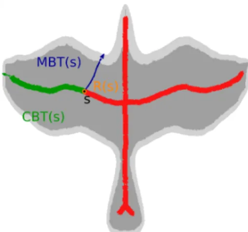
Figure 5: Depth functions at 3D curve skeleton point s: curve burn time CBT (s), medial burn time MBT (s) and radius R(s). To-gether they provide a global analysis of the shape around s, respec-tively depth, width and height (R(s) towards us).
Figure 6: The distance function D. In gray, two intersecting medial axis sheets belonging to the medial axis M. We distinguish the point m ∈ Mand s1and s2as two points on the skeleton C. The skeleton
lies on the medial axis. Despite s1being closer to m than s2in
Eu-clidean distance, (i.e., d(m, s1) < d(m, s2)), m will be associated to s2
because D(m, s2) < D(m, s1) (since MBT (m) − MBT (s2) ≈ d(m, s2)
and MBT (m) − MBT (s1) , d(m, s1)).
is the sum of the volumes assigned to the neigh-boring point in b that is closer to an extremity than s, together with the volumes of the tetrahedra as-signed to s.
Note that because MBT is not defined in the continuous setting [32], we cannot provide a continuous definition for WEDF.
4.3. Computing WEDF on the 3D curve skeleton In practice, 3D WEDF is computed for an input sur-face mesh, on a curve-skeleton consisting of points on the medial axis of the surface mesh. The sampling den-sity of the medial axis or skeleton points may affect the smoothness of the WEDF, but not its actual value.
Above, we discuss the volume T (s) assigned to a skele-tal point s. More precisely, T (s) is the sum of the vol-umes of the Delaunay tetrahedra whose circumcenters m ∈ Mare closest to s according to the following dis-tance function: D(m, s)= | M BT (m) − M BT ( s)| − d(m, s) (1) where d is the Euclidean 3D distance and MBT the me-dial burn time. Note that because MBT is defined only for discrete medial axes, we can define WEDF only in the discrete setting as well. Figure 4 shows the tetra-hedra and their circumcenters associated to a skeleton point s. Note that the proposed distance function D en-sures that a medial point m is necessarily contributing to a skeleton point s that lies on the same sheet of the medial axis, as illustrated in Figure 6.
The definition of T (s) ensures that points m associ-ated with s are lying along the burn path bs⊂ M
reach-ing the closest border of the medial axis accordreach-ing to the medial burning time. T (s) therefore measures the volume associated to all points on the burn path of s to the shape boundary, see Figure 4. By construction, each medial point m is associated to a unique skeleton point s. Taking Delaunay tetrahedra across all m ∈ M gives the volume of the entire shape, therefore taking T(s) across all s ∈ C partitions the shape volume into tetrahedra sets associated to each s ∈ C.
To compute WEDF values along the skeleton, we be-gin at a skeletal extremity and progress inward. Dur-ing the skeleton traversal, the WEDF value at a point is then computed from the value at the previous point: W EDF(s)= T(s) + WEDFprev (2)
W EDFprev= 0 at extremities; W EDF(y) if s is a regular point,
and y its neighbor with computed W EDF; P
i≥1
W EDF(yi) if s is a junction, and
all neighbors yibut one
y0have a WEDF value.
Here in equation (2), we define a summed WEDF, since at a junction s of the curve-skeleton the volume W EDF(s) is here the sum of values from all incoming skeleton branches. This differs from the 2D WEDF def-inition [5], where max values at branch junctions are taken. We use the summed WEDF because it is neces-sary to insure its robustness to surface noise. Indeed, with a 3D max-version of WEDF, small branches of the
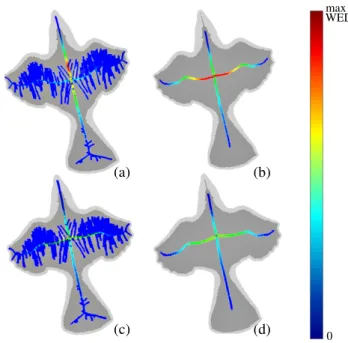
skeleton originating from noise would capture the vol-ume erroneously around them (by catching tetrahedra volume previously assigned to a main branch) and thus diminish the WEDF on the global shape. An illustration of the change in WEDF due to small branches is given by Figure 7. Conversely, in the summed version the vol-ume captured by the small branch is still contributing to the volume of the main branch, and therefore, WEDF values on main branches are stable.
(a) (b)
(c) (d)
max WEDF
0 Figure 7: Robustness of the summed WEDF. Two different curve skeletons for the same 3D shape, one with many branches(a,c)and a more filtered version with only main branches(b,d).
Top row(a,b): WEDF is computed by taking the max value of in-coming branches at intersections [6]. we observe a lack of robustness; the distribution of WEDF is different on the main branches of the two skeletons. In particular, the branch containing the greatest WEDF value is not the same.
Bottom row(c,d): our proposed summed WEDF computed by sum-ming WEDF values of incosum-ming branches at junctions. The distribu-tion of WEDF remains the same along the main branches of the skele-tons since the volume counted on small branches also contributes to the main branch value.
Figure 8 shows a color-coding of the WEDF function on curve skeletons for 3D objects. When the object and its curve skeleton have some symmetries, the WEDF re-mains symmetric. The WEDF value is maximum at a point whose value is the total volume within the surface of the object, and then decreases on any path towards curve skeleton extremities. As in 2D, WEDF along a skeleton path between two extremities is unimodal.
max WEDF
0 Figure 8: WEDF of 3D shapes. Low values are colored in dark blue high values in dark red. We can see that the WEDF grows slowly along branches that are surrounded by a limited volume (such as legs, arms, tail or finger) and grows faster on branches surrounded by an higher volume (belly or palm for instance).
5. Clustering the skeleton into parts according to salience
To demonstrate one avenue for application of our WEDF computation, we use the WEDF values defined on the skeleton to develop a salience measure for each point on the surface mesh. Examples of part salience on some well-known 3D shapes are shown in Section 7. 5.1. Partitioning skeleton points into salience levels
We perform unsupervised clustering on the WEDF values in order to identify parts at similar salience lev-els. The clustering we propose is a two-step process, where the first step determines the main shape of the skeleton and the second step identifies features with de-creasing saliency values. For a genus 0 surface mesh, the skeleton has a tree-like connectivity, where the root corresponds to the highest 3D WEDF value. Moving away from the root, the salience values monotonically decreases along the branches of the skeleton.
Identifying the main shape. We select main skeletal points as a subset of the skeletal points in two steps. On the 3D WEDF values, we perform a seeded k-means clustering with two clusters where the seeds are the min-imum and the maxmin-imum WEDF values of the junction skeletal points being clustered. We then associate all re-maining skeleton points to these two clusters based on their WEDF values. All skeletal points belonging to the
cluster with the centroid of largest WEDF value are se-lected as the main shape points.
Identifying features. The other 3D WEDF clusters are determined among those WEDF values of junction points and neighbors which are not in the main shape cluster: we again apply a k-means clustering with k in a given interval (in practice, we take k ∈ {2, 3, ..., 20}). An estimation of the best number of classes k is given by gap analysis [42]. Each cluster represents a salience level relevant for the shape. The level value L is cho-sen as the median WEDF value of the cluster: larger 3D WEDF values correspond to higher salience levels, i.e. closest to main shape, while lower values are less significant, corresponding to lower salience levels. Clustering skeleton points. The curve skeleton is par-titioned into clusters according to the clustering of its 3D WEDF values. We thus obtain a partition of the curve-skeleton into salience levels. Note that any path on the curve skeleton going from a point belonging to the main shape to an extremity point will traverse levels of salience in decreasing order, see Figure 9. This par-tial ordering of points of the curve skeleton, coherent with the tree topology of the medial axis, is the basis for the graded salience-based parts decomposition de-scribed in the next section.
This process allows cross-parts comparison of salience for all parts, and is therefore not restricted to those with junctions: for example, the thumb in the hand of Figure 9 is identified as a feature even if there is no junction in the curve skeleton, because its salience level matches the salience level of the other fingers.
6. Saliency measure for 3D shape surface decompo-sition and hierarchy
After having decomposed the skeleton into graded skeletal sub-parts (Fig.1-d), the second step of our method is transfer the parts decomposition to the shape’s surface, in order to partition the mesh into graded parts labeled by their salience (Fig.1-f).
This transfer is a challenging process. A naive method would map the cluster level of curve skele-ton points onto medial axis points using the distance function introduced for the computation of WEDF (see Equation (1) in Section 4.3). And, since each medial axis point is the circumcenter of a tetrahedra, assign-ing the cluster level value to its tetrahedra would di-rectly lead to a partition of the volume of the shape into cluster levels (Figure 4). However, it can be observed that lower level clusters, corresponding to features of
Figure 9: Decomposition of the curve-skeleton into graded salience levels, from main shape (dark red) to less significant parts (dark blue).
max WEDF
0
(a) (b)
Figure 10: The naive tetrahedra clustering(a)and our proposed clus-tering(b). We can see that the naive clustering gives a decomposition where sub-parts of lower saliency (like antennae or legs) are indeed entering into the parent shape of higher salience (here head or body). The naive tetrahedra clustering is therefore not sufficient.
lower salience, carve holes along the branches inside the parent shape: Delaunay tetrahedra whose circumcenters are medial points close to the center of the main shape may be associated to a curve skeleton point belonging to a lower level branch (we see this effect on the left image of Figure 10 where green triangles emerge from inside the main shape near attachment area of legs).
We therefore propose a two-step process to extend transfer salience levels from the skeletal points to the surface, using vertices instead of tetrahedra. We first as-sign each vertex of the surface a saliency level by con-sidering all medial points whose tetrahedra contain the vertex, and then determine a level value for the triangu-lar faces from the levels of the associated vertices. 6.1. Assigning salience levels to mesh vertices
We start with a surface mesh S and a curve skeleton C, where each skeletal point s is attributed a salience level L(s). Each s belongs to a cluster cluster(s), and
its associated level L= L(s), the median of the WEDF values within the cluster cluster(s). For each mesh ver-tex v ∈ S , we compute the skeleton point s, which is the closest to v using the following distance function:
F(v, s)= d(v, s)
L(s) (3)
with d(v, s) the Euclidean distance between v and s. This function warps the space to favor clusters of higher value: skeleton points belonging to high-level clusters have an F-distance smaller than the Euclidean distance to the mesh vertices, while skeleton points be-longing to clusters with lower value have an F−distance distance greater then the Euclidean distance to the mesh vertices. This way, curve-skeleton points belonging to higher salience-level clusters attract boundary points to the more significant part in terms of salience (body) rather than attaching to a less significant feature. See Fig.10, where mesh vertices are wrongly attached to the leg using the Euclidean distance (left), but correctly la-beled with a salience attached to the body (right).
6.2. Assigning salience levels to mesh faces
After this first step of assigning mesh vertices to salience levels of skeleton points, we label the mesh faces using the levels assigned to the three vertices be-longing to a face. If all vertices are assigned to the same level, we assign the face to this level, that is, the face salience value is the cluster salience. In salience tran-sition zones, where vertices of a face are assigned to different levels, we subdivide the face (1-4 subdivision) using points linearly interpolated on the three edges ac-cording to salience levels of the vertices, and assign lev-els to subregions accordingly. This generates a smooth transition between parts of the shape belonging to dif-ferent levels, as shown in the following experiments.
7. Experiments 7.1. Validation
First, Figure 11 shows the partition of different meshes created by considering each cluster on the skele-ton as a different part, without grouping by salience value. Note that the decomposition is coherent, and when the shape is close to symmetric, the decomposi-tion preserves this symmetry. Also observe that di ffer-ent parts, like the fingers of the hand, or the arms of the octopus, are well separated (thanks to the topology of the curve medial axis).
Figure 11: Shape segmentations based on our hierarchical decompo-sition; here each connected cluster on the curve skeleton generates a different part of the mesh partition.
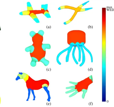
In Figure 12, we have now grouped parts according to salience, so each part with the same color has been de-termined to be at the same salience level. Moreover, be-cause the skeleton has a tree structure, the salience lev-els are monotonically decreasing from the main shape to the extremities of the shape, leading to a graded par-tition into subparts. We can see in all these results that the core of the shape is well-centered, while shape de-tails are localized at extremities. Also, the shape parts that are similar (legs, fins or antennas) are assigned to the same hierarchy level. The proposed segmentation then gives not only a partition of the shape, but also as-signs a level of salience to each feature that is global on the shape, and known to be consistent with perception in 2D [5, 33].
7.2. Robustness of the graded partition
We also recall that the proposed graded segmenta-tion is robust. First, computing the salience level on the curve skeleton reduces the instability of the medial axis to boundary noise. A curve skeleton may have a lot of small branches, or be simplified. We have seen in Figure 7 that the proposed computation of WEDF (sum-ming the inco(sum-ming values at junctions) provides stable WEDF values on the main branches, and thus insures a consistent segmentation. (a) (b) (c) (d) (e) (f) max WEDF 0
Figure 12: Shape decompositions on several shapes, with saliency-based partial ordering of the extracted sub-parts.The color of a part represents its centroid value. The main shape is often centered in the shape (a,b,c,e,f) or located at the part with greatest volume (d). Details and part of lowest saliency are at the extremities of the shapes (wings, ears, legs, fingers). While (a) and (e) are being decomposed in four levels, (b) is cut in three levels and (c), (d) and (f) only need two levels. Note the capacity of our approach to model shape with a medial axis close to the curve skeleton (e) but also shapes with no tubular parts (f) having a two dimensional medial sheet.
We also experiment with different curve skeletons as input. Curve skeletons are not uniquely defined for 3D objects, and the computation of a curve skeleton is not part of our work. Even though our method works suc-cessfully for different curve skeleton types, the qual-ity of the curve skeleton plays an important role, see Fig. 13. A good curve skeleton is well-centered and captures all small protrusions with branches associated to each feature (left) whereas a coarser skeleton leads to a coarser graded decomposition (right).
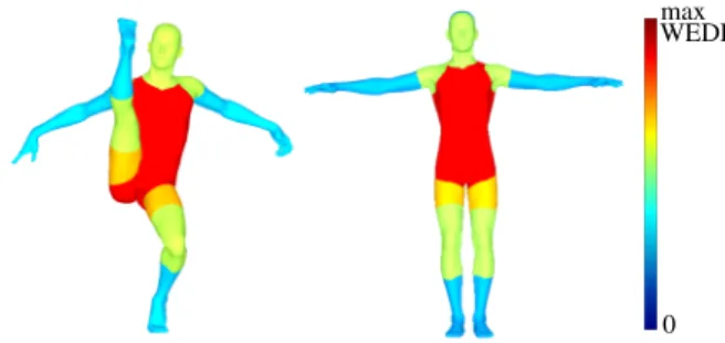
Figure 14 shows that our segmentation is naturally stable under constant volume shape deformation, since the WEDF measure generating the salience levels is vol-umetric. In other words, the salience levels stay consis-tent as moving parts articulate. The coloring between the two human figures remains consistent for the legs and arms, with only slight changes on the shoulders. Similarly, in Figure 15 the decomposition is very con-sistent across the different poses (a) to (d).
max WEDF
0
(a) (b)
(c) (d)
Figure 13: Comparison between two segmentations(a,b)using dif-ferent curve skeletons(c,d). The(a)decomposition uses the skeleton from [32], which is better centered and which correctly captures small protrusions (such as ears), while the first decomposition(b), uses the mean curvature skeleton(d)from [38], and is neither well-centered (see the tail) nor capturing correctly the small protrusions (such as ears). The(a)segmentation gives better results as small protrusions create smaller parts and as parts (legs, tail) are more finely cut, con-firming our preference for the skeleton (c).
8. Discussion and conclusion
We have produced a graded, salience-based parts par-tition from a importance measure on a curve skeleton of the shape integrating local PCA-like representation of a shape on the skeleton. Our method determines a level of relative importance for each sub-part, and la-bels features of the same salience level as belonging to a group with the same perceptual importance. More-over, because the decomposition respects the topology of the skeleton, it produces a parent-child relationship between parts in a given shape. At the highest level, the main shape contains the barycenter of the shape. Mov-ing away from the center, parts decrease in salience as a parent level gives way to a child. For genus 0 shapes, having a skeleton with tree structure, the parent of each part will be unique. As a result, the connectivity pro-duced by the skeleton allows for ordered parts relation-ships in a way that connectivity induced by cluster ad-jacency computed directly on the surface does not: for example, the ears of the horse on Fig. 12 have two adja-cent regions on the head, themselves neighbors, which would lead to a triangle connection (loop) between the three adjacent regions when using surface connectivity: skeletal connectivity results in two ears each connected
max WEDF
0 Figure 14: Stability of the segmentation relative to pose variation without change of topology.
to a head. Thus our decomposition is enriched by both a topological relationship between subparts, and an im-portance value attached to each subpart.
While our decomposition has consistent results on different curve skeletons, it still depends on the quality of the curve skeleton used to capture the shape. Indeed, as shown in Figs. 3 and 13, the results may vary depend-ing on the skeleton’s geometry and topology. However, for volume preserving deformation, the proposed de-composition is robust and gives a consistent labeling of the shape parts as long as the topology is preserved. As expected, the generalization of WEDF to 3D leads to an analysis of the shape that seems consistent with percep-tion, as shown in 2D in [5, 33]. Future work will include a user study to confirm the perceptual coherence.
In future work, we also plan to extend the present work in order to analyze the similarity between seg-mented parts belonging to the same salience level, by using for example a combination of PCA-like measures on the skeleton. This would enable to produce inputs to recent methods, such as SimSelect [4] or Pattern-Driven Colorization [43], where the user is required to annotate candidate similarities by hand.
Like in the 2D setting [33], our decomposition and salience could be validated by a user study asking to differentiate the different parts of a 3D object and tag the main shape, and the importance of each different part.
References
[1] G. H. Bower, A. L. Glass, Structural units and the redintegrative power of picture fragments., Journal of Experimental Psychol-ogy: Human Learning and Memory 2 (4) (1976) 456. [2] D. D. Hoffman, M. Singh, Salience of visual parts, Cognition
63 (1) (1997) 29–78.
[3] V. L´eon, N. Bonneel, G. Lavou´e, J.-P. Vandeborre, Continuous semantic description of 3d meshes, Computers & Graphics 54 (2016) 47–56.
[4] E. Guy, J.-M. Thiery, T. Boubekeur, Simselect: Similarity-based selection for 3d surfaces, Computer Graphics Forum 33 (2) (2014) 165–173.
max WEDF
0
(a) (b) (c) (d)
Figure 15: Several shape decompositions of a bird shape in different positions. The decomposition is stable under deformations. This part decomposition into saliency levels may therefore be used in animation.
[5] L. J. Larsson, G. Morin, A. Begault, R. Chaine, J. Abiva, E. Hu-bert, M. Hurdal, M. Li, B. Paniagua, G. Tran, et al., Identifying perceptually salient features on 2d shapes, in: Research in Shape Modeling, Springer, 2015, pp. 129–153.
[6] K. Leonard, G. Morin, S. Hahmann, A. Carlier, A 2d shape structure for decomposition and part similarity, in: 2016 23rd International Conference on Pattern Recognition (ICPR), 2016, pp. 3216–3221.
[7] A. Borji, L. Itti, State-of-the-art in visual attention modeling, IEEE transactions on pattern analysis and machine intelligence 35 (1) (2013) 185–207.
[8] L. Itti, C. Koch, E. Niebur, A model of saliency-based visual attention for rapid scene analysis, IEEE Transactions on pattern analysis and machine intelligence 20 (11) (1998) 1254–1259. [9] C. H. Lee, A. Varshney, D. W. Jacobs, Mesh saliency, in: ACM
transactions on graphics (TOG), Vol. 24, ACM, 2005, pp. 659– 666.
[10] R. Song, Y. Liu, R. R. Martin, P. L. Rosin, Mesh saliency via spectral processing, ACM Transactions on Graphics (TOG) 33 (1) (2014) 6.
[11] R. Song, Y. Liu, R. R. Martin, K. R. Echavarria, Local-to-global mesh saliency, The Visual Computer (2016) 1–14.
[12] A. Nouri, C. Charrier, O. L´ezoray, Multi-scale mesh saliency with local adaptive patches for viewpoint selection, Signal Pro-cessing: Image Communication 38 (2015) 151–166.
[13] D. H. Kim, I. D. Yun, S. U. Lee, A new shape decomposi-tion scheme for graph-based representadecomposi-tion, Pattern Recognidecomposi-tion 38 (5) (2005) 673–689.
[14] X. Chen, A. Saparov, B. Pang, T. Funkhouser, Schelling points on 3d surface meshes, ACM Transactions on Graphics (TOG) 31 (4) (2012) 29.
[15] P. Theologou, I. Pratikakis, T. Theoharis, A comprehensive overview of methodologies and performance evaluation frame-works in 3d mesh segmentation, Computer Vision and Image Understanding 135 (2015) 49–82.
[16] Z. Xie, K. Xu, L. Liu, Y. Xiong, 3d shape segmentation and la-beling via extreme learning machine, Computer graphics forum 33 (5) (2014) 85–95.
[17] H. Benhabiles, G. Lavou´e, J.-P. Vandeborre, M. Daoudi, Learning boundary edges for 3d-mesh segmentation, Computer Graphics Forum 30 (8) (2011) 2170–2182.
[18] Y.-K. Lai, S.-M. Hu, R. R. Martin, P. L. Rosin, Rapid and ef-fective segmentation of 3d models using random walks, CAGD 26 (6) (2009) 665–679.
[19] F. Bergamasco, A. Albarelli, A. Torsello, A graph-based tech-nique for semi-supervised segmentation of 3d surfaces, Pattern Recognition Letters 33 (15) (2012) 2057–2064.
[20] Y. Fang, M. Sun, M. Kim, K. Ramani, Heat-mapping: A robust approach toward perceptually consistent mesh segmentation, in:
IEEE Computer Vision and Pattern Recognition (CVPR), 2011, pp. 2145–2152.
[21] O. K.-C. Au, Y. Zheng, M. Chen, P. Xu, C.-L. Tai, Mesh seg-mentation with concavity-aware fields, IEEE Transactions on Visualization and Computer Graphics 18 (7) (2012) 1125–1134. [22] S. Pulla, A. Razdan, G. Farin, Improved curvature estimation for watershed segmentation of 3-dimensional meshes, IEEE Trans. on Visualization and Computer Graphics 5 (4) (2001) 308–321. [23] A. Koschan, Perception-based 3d triangle mesh segmentation using fast marching watersheds, in: Computer Vision and Pat-tern Recognition, Proceedings, Vol. 2, IEEE, 2003, pp. II–27. [24] S. Berretti, A. Del Bimbo, P. Pala, 3d mesh decomposition using
reeb graphs, Image and Vision Computing 27 (10) (2009) 1540– 1554.
[25] S. Biasotti, D. Giorgi, M. Spagnuolo, B. Falcidieno, Reeb graphs for shape analysis and applications, Theoretical Com-puter Science 392 (2008) 5–22.
[26] T. El-Gaaly, V. Froyen, A. Elgammal, J. Feldman, M. Singh, A bayesian approach to perceptual 3d object-part decomposi-tion using skeleton-based representadecomposi-tions, in: Proceedings of the Twenty-Ninth AAAI Conference on Artificial Intelligence, AAAI Press, 2015, pp. 3762–3768.
[27] X. Li, T. W. Woon, T. S. Tan, Z. Huang, Decomposing polygon meshes for interactive applications, in: Proceedings of the 2001 symposium on Interactive 3D graphics, ACM, 2001, pp. 35–42. [28] J. Kustra, A. Jalba, A. Telea, Shape segmentation using medial point clouds with applications to dental cast analysis, in: Proc. of the 9th Int. Conf. on Computer Vision Theory and Applica-tions (VISAPP 2014), 2014, pp. 162–170.
[29] C. Feng, A. C. Jalba, A. C. Telea, Part-based segmentation by skeleton cut space analysis, in: Int. Symposium on Mathemati-cal Morphology and Its Applications to Signal and Image Pro-cessing, Springer, 2015, pp. 607–618.
[30] J. Tierny, J.-P. Vandeborre, M. Daoudi, Topology driven 3d mesh hierarchical segmentation, in: Shape Modeling and Ap-plications, 2007. SMI’07. IEEE International Conference on, IEEE, 2007, pp. 215–220.
[31] L. Liu, E. W. Chambers, D. Letscher, T. Ju, Extended grassfire transform on medial axes of 2d shapes, CAD 43 (11) (2011) 1496–1505.
[32] Y. Yan, K. Sykes, E. Chambers, D. Letscher, T. Ju, Erosion thickness on medial axes of 3d shapes, ACM Trans. on Graphics 35 (4) (2016) 38:1–38:12.
[33] A. Carlier, K. Leonard, S. Hahmann, G. Morin, M. Collins, The 2d shape structure dataset: A user annotated open access database, Computers & Graphics 58 (2016) 23–30.
[34] T. K. Dey, J. Sun, Defining and computing curve-skeletons with medial geodesic function, in: Symposium on geometry process-ing, Vol. 6, 2006, pp. 143–152.
[35] J. Giesen, B. Miklos, M. Pauly, C. Wormser, The scale axis transform, in: Proceedings of the twenty-fifth annual sympo-sium on Computational geometry, ACM, 2009, pp. 106–115. [36] N. Amenta, M. Bern, M. Kamvysselis, A new voronoi-based
surface reconstruction algorithm, in: Proceedings SIGGRAPH, ACM, 1998, pp. 415–421.
[37] A. Tagliasacchi, T. Delame, M. Spagnuolo, N. Amenta, A. Telea, 3D Skeletons: A State-of-the-Art Report, Computer Graphics Forum 35 (2) (2016) 573–597.
[38] A. Tagliasacchi, I. Alhashim, M. Olson, H. Zhang, Mean curva-ture skeletons, Computer Graphics Forum 31 (5) (2012) 1735– 1744.
[39] T.-C. Lee, R. L. Kashyap, C.-N. Chu, Building skeleton models via 3-d medial surface axis thinning algorithms, CVGIP: Graph-ical Models and Image Processing 56 (6) (1994) 462–478. [40] M. Livesu, F. Guggeri, R. Scateni, Reconstructing the
curve-skeletons of 3d shapes using the visual hull, IEEE transactions on visualization and computer graphics 18 (11) (2012) 1891– 1901.
[41] M. Livesu, R. Scateni, Extracting curve-skeletons from digital shapes using occluding contours, The Visual Computer 29 (9) (2013) 907–916.
[42] R. Tibshirani, G. Walther, T. Hastie, Estimating the number of clusters in a data set via the gap statistic, Journal of the Royal Statistical Society: Series B (Statistical Methodology) 63 (2) (2001) 411–423.
[43] G. Leifman, A. Tal, Pattern-driven colorization of 3d surfaces, in: 2013 IEEE Conference on Computer Vision and Pattern Recognition, 2013, pp. 241–248.
![Figure 3: Medial axis (dark gray) and a curve skeleton (yellow) of a 3D shape. The medial axis is obtained using [35] and curve skeleton using [32]](https://thumb-eu.123doks.com/thumbv2/123doknet/14380978.506127/6.892.461.798.164.348/figure-medial-curve-skeleton-yellow-medial-obtained-skeleton.webp)