Computational treatments for neutron resonance elastic scattering in Monte Carlo nuclear simulations

Computational Treatments for Neutron Resonance Elastic

Scattering in Monte Carlo Nuclear Simulations

by

Vivian Y. Tran

SUBMITTED TO THE DEPARTMENT OF NUCLEAR SCIENCE AND

ENGINEERING IN PARTIAL FULFILLMENT OF THE

REQUIREMENTS FOR THE DEGREE OF

BACHELOR OF SCIENCE IN NUCLEAR SCIENCE AND

ENGINEERING AT THE

MASSACHUSETTS INSTITUTE OF TECHNOLOGY

June 2016

© 2016 Vivian Y. Tran. All rights reserved.

The author hereby grants to MIT permission to reproduce and to distribute publicly paper and electronic copies of this thesis document in whole or in part.

Signature of Author:_____________________________________________

Vivian Y. Tran Department of Nuclear Engineering May 18, 2016

Certified by:___________________________________________________

Benoit Forget Associate Professor of Nuclear Science and Engineering Thesis Supervisor

Accepted by:___________________________________________________

Michael P. Short Assistant Professor of Nuclear Science and Engineering Chairman, Committee for Undergraduate Students

Computational Treatments for Neutron Resonance Elastic

Scattering in Monte Carlo Nuclear Simulations

by

Vivian Y. Tran

Submitted to the Department of Nuclear Science and Engineering on May 18, 2016 In partial Fulfillment of the Requirements for the Degree of

Bachelor of Science in Nuclear Science and Engineering

ABSTRACT

Simulations are vital to the safe design and operation of nuclear reactors. It is therefore important that they accurately treat the physics of nuclear interactions. This work

investigates the phenomenon of neutron resonance scattering with a moving target, which can affect the post-collision properties of the neutron and macroscopic values such as temperature reactivity coefficients. First, this research validates a faster computational treatment for resonance scattering--the accelerated resonance elastic scattering (ARES) kernel sampling method--against the already verified Doppler broadening rejection correction (DBRC) treatment in the open-source OpenMC Monte Carlo neutron transport code being developed at the Massachusetts Institute of Technology. In an effort to

improve computational efficiency, the optimal energy limits where this phenomenon should be treated are determined and compared to the less costly but inaccurate

approximation of assuming a constant constant cross section for determining the reaction kinematics. To reduce memory requirements and facilitate coupling with heat transfer, a new data representation was recently adopted in OpenMC based on the multipole

formalism. However, this new approach invalidates the previous implementations of DBRC and ARES. This thesis thus developed a modified DBRC algorithm compatible with the new data representation. This new method is also validated against the previous DBRC method. While more computationally costly, the use of the multipole

representation in treating resonance scattering reduces memory requirements by a hundred-fold and facilitates the representation of temperature dependent cross sections.

Thesis Supervisor: Benoit Forget

Acknowledgements

First, I would like to thank my graduate student mentor, Jonathan Walsh, who introduced me to the project two years ago and guided me through it from beginning to end. After participating in 6 other research projects during my time at MIT, I can genuinely say that he has been a wonderful mentor. He was always willing to explain new concepts and spend extra hours debugging code, provided me the vision and guidance needed to move on to the next step, and was overall pleasant and extremely productive to work with. I also want to express my gratitude to my research advisors, Professors Ben Forget and Kord Smith. Their support throughout this research, from organizing UROP presentations to meeting one-on-one to discuss progress and share their extensive knowledge, have been an enormously motivating and produtive part of getting this work done. Prof. Forget has especially challenged me to dive more fully into the underlying physics of this work, effectively sharing his enthusiasm for the field and making the project more meaningful and enjoyable for me. He has also been an essential part of the editing of this document. I also thank Colin Josey for his collaboration on developing new resonance treatments compatible with the windowed multipole method. Without the productive conversations with him, and not to mention his own work on the multipole representation, an essential part of this research would not have been possible.

Finally, thanks also to the Nuclear Science and Engineering Department, which has provided many of the cups of coffee and friendship needed to complete this work.

Contents

Abstract 3 Acknowledgements 5 Table of Contents 7 List of Figures 9 List of Tables 10 1. Introduction 11

1.1 Motivations and Objections 11

1.2 Arrangement of Thesis 11

2. Background 12

2.1 OpenMC Particle Transport Code 12

2.2 Neutron Resonance Elastic Scattering 13

2.3 Current Cross Section Representation in OpenMC 19

2.4 Multipole Formalism 22

3. Methods - Computational Treatments for Resonance Scattering 26

3.1 Constant Cross Section (CXS) Approximation 26

3.2 Doppler Broadening Rejection Correction (DBRC) Method 28

3.3 Accelerated Resonance Elastic Scattering (ARES) Kernel Sampling Method 30

3.4 New DBRC-Multipole Methods 32

3.4.1 DBRC-MP-Global Method 33

3.4.2 DBRC-MP-Local Method 33

4. Results - Validation of ARES 35

4.1 Scattering Kernels 36

4.2 Average Energies After Scattering 37

4.3 Upscattering Probabilities 37

5. Results - Energy Intervals to Apply DBRC and ARES 39

5.1 Determining Energy Intervals Based on Eigenvalue Calculations 39

5.2 Verification of Determined Energy Intervals 42

6. Results - Verification and Comparison of DBRC-Multipole Methods 44

6.3 Upscattering Probabilities 47

6.4 Computation Time 47

6.5 Eigenvalue Calculations 49

7. Conclusions and Future Work 51

7.1 Conclusions 51

7.2 Future Work 51

8. Appendix 52

8.1 Detailed Scattering Kernels for DBRC-MP Methods 53

8.2 Detailed Fixed Source Single Scattering With DBRC-MP Run Data 56

List of Figures

Figure 2.1-1: Layout of Fuel Assemblies 13

Figure 2.2-1: Resonance Energy Levels 15

Figure 2.2-2: Cross Sections for H-1 and H-2 15

Figure 2.2-3: Cross Section for U-238 16

Figure 2.2-4: Doppler Broadening of Resonance at Different Temperatures 17

Figure 2.2-5: Illustration of Exact Scattering Kernel 18

Figure 2.2-6: Illustration of Asymptotic Scattering Kernel 18

Figure 2.2-7: Ghrayeb's Scattering Kernel for U-238 at 6.52 eV 19

Figure 2.3-1: Total Microscopic Cross Section for H-1 Doppler Broadened to 293.6 K 21

Figure 2.3-2: Total Microscopic Cross Section for U-238 Doppler Broadened to 293.6 K 21

Figure 2.3-3: Two Doppler Broadened Resonances 22

Figure 2.4-1: Construction of Windows in WMP Formulation 26

Figure 3.2-1: Visual Representation of Rejection Sampling by DBRC 29

Figure 3.3-1: Visual Representation of Rejection Sampling by ARES 32

Figure 4-1: Pin Cell with Reflective Boundary Conditions 35

Figure 4.1-1: 900 K Scattering Kernel for U-238 at 36.25 eV 36

Figure 4.1-2: 900 K Scattering Kernel for U-238 at 65.23 eV 36

Figure 5.1-1: Differences in keff at Various Energies for U-238 40

Figure 5.1-2: Differences in keff at Various Energies for U-235 40

Figure 5.1-3: Differences in keff at Various Energies for Sn-119 40

Figure 6.1-1: 600 K Scattering Kernel for U-238 at 6.52 eV 45

Figure 6.1-2: 600 K Scattering Kernel for U-238 at 20.2 eV 45

Figure 6.1-3: 600 K Scattering Kernel for U-238 at 36.25 eV 46

Figure 8.1-1: 600 K Scattering Kernel of U-238 at 6.52 eV with DBRC-MP-Global 53

Figure 8.1-2: 600 K Scattering Kernel of U-238 at 6.52 eV with DBRC-MP-Local 54

Figure 8.1-3: 600 K Scattering Kernel of U-238 at 20.2 eV with DBRC-MP-Global 54

Figure 8.1-4: 600 K Scattering Kernel of U-238 at 20.2 eV with DBRC-MP-Local 55

Figure 8.1-5: 600 K Scattering Kernel of U-238 at 36.25 eV with DBRC-MP-Global 55

List of Tables

Table 4.2-1: Average Energies after Scattering in the Vicinity of Resonance for

U-238 at 900 K 37

Table 4.3-2: Probabilities of Neutron Upscattering Near S-Wave Resonance Energies

for U-238 38

Table 5.1-1: Energy Ranges to Apply Resonance Corrections for Each Resonant

Nuclide 41

Table 5.2-1: keff Values From Simulating All Resonant Nuclides in the BOC-HZP

Pin Cell 42

Table 6.2-1: Average Energies after Scattering for U-238 Using Various DBRC

Methods 47

Table 6.3-1: Upscattering Probabilities for U-238 Using Various DBRC Methods 47

Table 6.4-1: Computation Times for Fixed Source Simulations with Resonance

Scattering Treatments 48

Table 6.4-2: Computation Times for Fixed Source Simulations without Scattering 48

Table 6.5-1: Eigenvalue Calculations at 600 K Using Various DBRC Methods 49

Table 6.5-2: Eigenvalue Calculations at 900 K Using Various DBRC Methods 50

1

Introduction

1.1 Motivations and Objectives

Modelling and simulation is an essential part of the design and safe operation of nuclear reactors, and it is thus important that the physics at hand are accurately represented. This thesis focuses on the computational treatments for resonance elastic scattering in the OpenMC code [1].

The resonance scattering phenomenon, in which the scattering cross sections of resonant nuclides can vary drastically within small energy intervals, is an important physics consideration, as it can affect macroscopic values such as temperature reactivity coefficients. Past simulations have properly Doppler broadened the resonant nuclide cross-section, but failed to capture the proper kinematics (i.e. outgoing energy and angle). Most common methods developed to capture the proper kinematics of the resonant scattering kernel are computationally expensive, but recent work aimed at accelerating the process [2]. This new method is validated in this research. This thesis also seeks to determine the energy limits at which correct treatment is necessary in an effort to improve computational efficiency without loss of accuracy.

Another goal of this work is to develop and test a new algorithm for the treatment of resonance scattering in the presence of a moving target compatible with a new cross section representation in Monte Carlo simulations. The most commonly used cross section representation for Monte Carlo simulations is based on the ACE format which relies on storing pointwise cross section data that can be linearly interpolated in energy and temperature which proves costly when modelling a system with a detailed temperature profile. Such calculations require an enormous amount of nuclear data which often exceeds node memory of modern computing platforms. To this end, OpenMC has recently adopted the multipole representation of nuclear data [3], which is a physical model that can be evaluated directly at the desired energy and temperature, and developed an efficient adaption known as the Windowed Multipole (WMP) Method [4]. However, this new format is incompatible with current resonance correction methods that rely on the pointwise nature of the data. In this thesis, a new algorithm for treating resonance scattering using the multipole representation is developed and tested.

1.2 Arrangement of Thesis

This thesis is arranged as follows: 1. Introduction

2. Background 3. Methods

4. Validation of ARES

5. Limiting application of correct resonance treatments 6. Implementation of DBRC+Mulitpole

2

Background

2.1 OpenMC Particle Transport Code

OpenMC is an open-source Monte Carlo neutron transport code that has been under active development at the Massachusetts Institute of Technology by the Computational Reactor Physics Group since early 2011 [2].

Monte Carlo methods rely on repeated random sampling of physcaillty derived probabitlity distribution functions to obtain numerical results. Because of their probabalistic nature, Monte Carlo simulations are useful for modeling systems such as nuclear reactors, where neutrons are moving randomly about. Neutrons are especially important in nuclear systems because they induce fission in uranium and other nuclides. Modelling the behavior of neutrons makes it possible to figure out the distribution of neutrons in the core, and more importantly the distribution of energy produced. By simulating many neutrons, the average behavior of these particles can be determined very accurately. From this, important characteristics of the system such as the pin powers, fuel temperature, clad temperature, reactivity coefficients, amount of poison needed to maintain criticality, etc. can be determined and used to help design and safely operate nuclear reactors [5].

OpenMC allows users to build models and run simulations of nuclear reactor cores and other nuclear systems, as shown in Fig. 2.1-1. At present, this code is capable of simulating neutrons in either fixed source or eigenvalue problems. OpenMC can faithfully simulate all nuclear reactions producing secondary neutrons. It allows for high-fidelty simulations through constructive solid geometry representation and continuous-energy physics. Other features include plotting, coarse mesh finite difference acceleration, and variance reduction [6].

Many legacy codes do not scale well on existing and future parallel computer architectures. As a relatively new Monte Carlo particle transport code, OpenMC development was focused on using modern software design practices and high performance scalable algorithms to enable high-fidelity, large-scale simulations. OpenMC is currently capable of scaling up to hundreds of thousands of processors [2]. OpenMC has been shown to have excellent accuracy and scalability in criticality benchmark and full core eigenvalue calculations. OpenMC has been validated against a selection of benchmarks part of the International Criticality Safety Benchmark Evaluation Project (ICSBEP) [7], as well as the full core Benchmark for Evaluation and Validation of Reactor Simulations (BEAVRS) [8]. Results obtained from OpenMC simulations have also been shown to agree well with those obtained from MCNP5 [9].

OpenMC can be found online via github [10], and its documentation is available on the CRPG website [11].

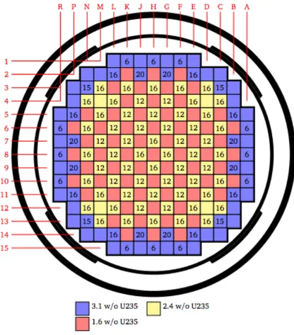
Fig. 2.1-1 Layout of Fuel Assemblies

This layout is taken from BEAVRS full core benchmark, to demonstrate the modeling capabilities of OpenMC [12]

2.2 Neutron Resonance Elastic Scattering

Elastic scattering is a neutron-nuclide interaction that is essential to the neutron slowing down process in which neutrons lose energy and eventually enter the thermal energy range from which the majority of neutron-induced fission events occur. The probability of such an interaction can be described by the neutron scattering cross section of the nuclide, which varies with energy and temperature.

In elastic scattering, a neutron collides with a target nuclei and bounces off. The overall interaction conserves momentum and energy, but energy from the neutron may be transferred to the target nuclei.

If the target is at rest, the energy of the neutron after scattering can be described by 𝐸′ = (!!!) ! (!!!) !"#(!!)

where 𝐸' is the energy after the elastic scattering event, 𝜃_! is the angle between the incoming neutron's trajectory and the scattered nuclei, E is the incoming neutron's kinetic energy, and

𝛼 = !!!_!!! !,

where A is the atomic mass number of the target nuclei [13].

While the assumption that the target nuclei is at rest can be used to accurately model elastic scattering events when the incoming neutron energy is sufficiently high, this is not true in the epithermal energy range. In this range, the thermal motion of the target nuclide can have a significant effect on the scattering kernels [2, 13].

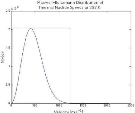
Typically, stochastic treatments commonly make the assumption that target speeds can be modelled as an isotropic Maxwell-Boltzmann ideal gas. When determining the outgoing energy and angle, the simplifying assumption is often made that the cross section is constant over the narrow range of probable neutron energies, which is an inadequate approximation for heavy nuclides with resonances [2, 13].

Resonant nuclides have scattering cross sections that can vary drastically within small energy intervals. These cross section peaks are called resonances, and each one manifests due to a particular compound (or excited) state of the nucleus. The resonance scattering cross section can be modeled approximately by the single-level Breit-Wigner (SLBW) formula (for illustrative purposes, more complex models are often used in simulations):

𝜎_! 𝑥 = 2 Γ 𝑟𝜓 𝑥 + 𝑞𝜒 𝑥 + 𝜎! 𝑥 = 2 𝐸 − 𝐸_Γ ! 𝜓 = 1 1 + 𝑥! 𝜒 = 2𝑥 1 + 𝑥!

where Γ is the resonance width (in eV) at half-peak.

The formation of resonances is due to the quantum nature of nuclear forces. Nuclear reactions are essentially transitions between different discrete quantum energy levels. If the relative energy between the nucleus and an incoming particle is equal to a compound nucleus at one of the excitation states, a resonance can be created and a peak occurs in the cross section, as illustrated in Fig. 2.2-1.

Fig 2.2-1 Resonance Energy Levels

Energy levels of the compound nucleus translate to resonances, and when the projectile (neutron) and target nuclei have a relative energy very close to one of these energy levels,

resonance peaks in the cross section can be seen [14]

Fig 2.2-2 Cross Section for H-1 and H-2

Elastic scattering cross sections are shown for H-1 in red and H-2 in green. These two nuclides exhibit no resonances [13]

Light nuclides have lower allowable state densities and the distance between states is larger than heavy nuclides [14]. Of all nuclides, only hydrogen and deuterium exhibit no resonances [15], as shown in Fig. 2.2-2 [13]. This translates to larger resonance regions for heavy nuclides. For heavy nuclides, resonances appear at much lower energies and have very narrow widths compared to lighter nuclides. The resonance region for U-238 is shown in Fig. 2.2-3. [12]

Fig 2.2-3. Cross Section for U-238

The resonance region contains many sharp peaks [14]

In neutron resonance elastic scattering, the neutron collides with the resonant target nuclei with a relative energy in the vicinity of a resonance. In this interaction, the neutron penetrates the nucleus and creates a compound nucleus, which is in an excited state. The compound nucleus regains stability by decaying, or emitting a neutron. The emitted neutron is not necessarily the same one that initially collided. [16, 17].

Because the neutron cross section depends on the relative velocity between the neutron and nuclide, the Doppler effect arises. When the target nucleus is in thermal motion, the impinging neutron appears to have a continuous spread in energy. This effectively changes the observed shape of the resonance, causing it to broaden the energy range of neutrons that may be resonantly absorbed or scattered. The resonance cross section becomes shorter and wider than it is when the target nuclei are at rest (or at 0 K). Though the shape of the resonance changes with temperature, the total area under it remains constant. An illustration of Doppler broadening is shown in Fig. 2.2-4 [16]. Doppler broadening of resonances can affect fuel temperature coefficients and average energies

after scattering [18]. At higher temperatures, neutrons have a higher chance of

upscattering after a resonance elastic scattering interaction. For instance, the upscattering probability for an incident neutron with 20.2 eV on U-238's 20.67 eV resonance increases from about 5% at 300 K to 30% at 1000 K [19].

Fig 2.2-4 Doppler Broadening of Resonances at Different Temperatures

At higher temperatures (T3) the resonance cross section gets flattened out [16]

In the past, the fact that the loss of energy by neutrons is the dominant energy exchange mechanism for very fast neutrons led to the widespread use of the approximation that the gain of energy by neutrons in collisions with lattice atoms was negligible above the thermal range [19]. This assumption was first proven to be inaccurate in the vicinity of large scattering resonances in 1991 [20]. It is now known that the resonance scattering phenomenon can bias the secondary angle-energy distribution of scattered neutrons if insufficient detail is preserved in the physical model used to describe it. These biases can affect integral results such as reaction rates and reactivity [21]. Past research has further shown that the exact scattering kernel increases LWR Doppler coefficients by roughly 10% compared to the commonly used asymptotic model which assumes the target nuclei is at rest. This difference results in a decrease in the hot full power eigenvalues by roughly 200 pcm for LWRs [22].

To illustrate, the exact kernel is shown in Fig. 2.2-5 and the asymptotic kernel is shown in Fig. 2.2-6.

Fig. 2.2-5 Illustration of Exact Scattering Kernel The thermal motion of the target nuclide is account for [13]

Fig. 2.2-6 Illustration of Asymptotic Scattering Kernel

In the asymptotic model, the target nuclide is presumed to be at rest [13]

Ouislouman and Sanchez first derived the formula of the moments for energy transfer kernels from elastic scattering events, accounting for lattice interactions in which the scattering neutron may lose or gain energy from the interaction. 𝜎_!"! _{(𝐸 → 𝐸′) = 𝛾 𝑡𝜎} !!"# 𝛽 𝑘𝑇 𝐴 𝑡! ! ! 𝑒!! ! !𝜓_!(𝑡)𝑑𝑡 where 𝛾 = 𝛽 ! ! 4𝐸𝑒 ! !" where t is a variable proportional to the neutron speed, and 𝛽 is defined as 𝛽 = 𝐴 + 1 𝐴 where A is the atomic mass number of the lattice atoms, k is Boltzmann's constant, and T is the temperature of the lattice.

𝜓_!(𝑡) is the nth order component of the angular dependence of the scattering kernel. 𝜎_!!"# _{is the tabulated cross section values at 0 K [20].}

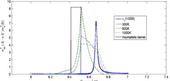
Recently in 2011, Ghrayeb applied this deterministic approach to anisotropic scattering cases and produced numerical results for the scattering kernels, some of which are relevant to this research. Ghrayeb's scattering transfer kernels at 6.52 eV, just below the first resonance of U-238, is reproduced below in Fig. 2.2-7 [19].

Results from this thesis focusing on computational treatments for resonance scattering using Monte Carlo methods will be compared with those from Ghrayeb's deterministic approach. Fig. 2.2-7 Ghrayeb's Scattering Kernel for U-238 at 6.52 eV The effective scattering transfer kernel of U238 is shown at various temperatures just below the 6.67 eV resonance for neutrons of energy 6.52 eV [19]

2.3 Current Cross Section Representation in OpenMC

Currently in OpenMC, nuclear data governing the interaction of neutrons with various nuclei are represented using the ACE format [23, 24]. This format is also used by the MCNP and Serpent codes. These data files contain point-wise continuous-energy cross-section data in ACE format for elastic scattering reactions, fission reactions, inelastic scattering reactions, and other absorption reactions, as well as secondary angular and energy information. The files also include probability tables in the unresolved resonance range if applicable [24].

ACE-format data can be generated with the NJOY processing system which converts raw ENDF/B data into linearly interpolable data as required by most Monte Carlo codes. The use of a standard cross section format allows for a direct comparison of OpenMC with other codes since the same cross section libraries can be used [23].

With this format, continuous energy cross sections for each nuclide in a problem are stored as a function of energy, and this method can have a substantial effect on the performance of a Monte Carlo simulation. Each nuclide has cross sections tabulated over a wide range of energies, since the ACE format is based on linearly-interpolable cross sections. Therefore, while some nuclides may only have a few points tabulated (such as H-1, which has 590 tabulated energy points at room temperature of 293.6 K), other nuclides may have thousands of points tabulated (such as U-238, which is extremely important when considering resonance scattering and has 219456 tabulated energy points at room temperature) [23].

To account for temperature dependence, Doppler broadening is done numerically on these files. The nuclear data is often pre-processed and stored at many temperatures, with sufficiently small temperature spacing to preserve accuracy, and then interpolated. Past research by Trumbull has shown that cross sections can be interpolated within an accuracy of 0.1% over a temperature interval of 111 K for H-1, B-10, and O-16. For nuclides with more complex resonance behavior, smaller intervals are required. For natural Zr, U-238, and U-235, some values of the interpolated cross sections remained greater than 0.1% relative difference even with a 28 K temperature interval. For these nuclides, even smaller temperature spacing for interpolation is necessary [25]. Because these heavier nuclides already have many more points tabulated in the ACE format than light nuclides, the extra temperature interpolation, including pre-processing and storage, further increases memory requirements.

The total cross section Doppler broadened to room temperature for H-1 is included in Fig. 2.3-1 and for U-238 in Fig. 2.3-2. To further demonstrate the effect of and need for Doppler broadening for resonances, the effects of Doppler broadening on two resonances of U-238 from 293.6 K to 811 K is shown in Fig 2.3-3 [25]. As mentioned earlier and illustrated in the figure, Doppler broadening of resonances flattens and widens the peak at higher temperatures compared to lower temperatures, but the area under the curve remains the same.

Fig 2.3.1 Total Microscopic Cross Section for H-1 Doppler Broadened to 293.6 K [25]

Fig 2.3-2 Total Microscopic Cross Section for U-238 Doppler Broadened to 293.6 K [25]

Fig 2.3-3 Two Doppler Broadened Resonances

Effects of Doppler broadening on two resonances of the U-238 total microscopic cross section from 293.6 K to 811 K is illustrated [25]

2.4 Multipole Formalism

In addition to the ACE-format of the usual pointwise representation of cross sections, OpenMC also supports a relatively new experimental nuclear data format, called the windowed multipole method (WMP) [4, 26], in which cross sections are represented by sets of poles and residues [3]. This format requires less memory and allows on-the-fly Doppler broadening of cross sections to arbitrary temperatures. The WMP method has recently been implemented and verified in OpenMC, providing a simple way of computing nuclear data at any temperature, which is essential for multi-physics calculations [4].

The multipole representation of cross sections was first proposed by Hwang [3], and it works by transforming resonance parameters into a set of poles, 𝑝_!, and residues, 𝑟_!. The multipole formalism is a mathematically exact alternate representation of Reich-Moore and Multi-Level Breit-Wigner data.

In the multipole form, the cross sections are represented by sums of poles and residues. For each set of quantum numbers, there is a corresponding set of resonance levels. Each of these resonance levels can be decomposed into a sum of poles and residues [4].

The 0 K cross sections in the resolved resonance is computed by summing up the contribution from each pole [4, 5, 26]:

𝜎(𝐸, 𝑇 = 0 𝐾) = 1 𝐸 𝑅𝑒 𝑖𝑟_! 𝐸 − 𝑝_! ! Let 𝑧 = !!!! ! ! , 𝜉 = !!!

!!, and 𝑢 = 𝐸. Assuming free-gas thermal motion, cross

sections in the multipole form can be analytically Doppler broadened: 𝜎(𝐸, 𝑇) = 1 2𝐸 𝜉 𝑅𝑒 𝑖𝑟! 𝜋𝑊!(𝑧) − 𝑟! 𝜋𝐶 𝑝! 𝜉, 𝑢 2 𝜉 ! with 𝑊_!(𝑧) = _!! _!!! 𝑑𝑡!_!!!!!!, and 𝐶 !! !, ! ! ! = 2𝑝! 𝑑𝑢 ! !!(!!!!)!/!! !_!!!!!" ! ! ,

where T is the temperature of the resonant nuclide, 𝑘_! is the Boltzmann constant, and A is the atomic mass number of the target nucleus. The ability to analytically evaluate the Doppler broadened cross sections is the key advantage to the multipole formalism. [23] For the case that 𝐸 ≫ 𝑘_!T/A, 𝐶 !!

!, !

! ! is approximately zero, simplifying the

multipole cross section to

𝜎(𝐸, 𝑇) = 1

2𝐸 𝜉 _! 𝑅𝑒 𝑖𝑟! 𝜋𝑊!(𝑧)

The 𝑊!(𝑧) integral can be simplified down to analytic form, and we define the Faddeeva

function, 𝑊, as:

𝑊 𝑧 = 𝑒!!!

𝐸𝑟𝑓𝑐 −𝑖𝑧 Through this, the integral transforms as:

𝐼𝑚 𝑧 < 0 ∶ 𝑊_! 𝑧 = −𝑊 𝑧∗ ∗

There already exist algorithms to evaluate the Faddeeva function. For many nuclides, the Faddeeva function needs to be evaluated thousands of times to calculate a cross section. To mitigate the computational cost, the windowed multipole (WMP) method only evaluates poles within a certain energy "window" around the incident neutron energy and accounts for the effect of resonances outside that window with a polynomial fit, which can also be broadened exactly. This exact broadening can make up for the removal of the C integral. Typically at low energies, only curve fits are used. [4, 26] This windowing method is illustrated in Fig. 2.4-1. [4]

Fig 2.4-1 Construction of Windows in WMP Formulation [4]

The implementation of WMP in OpenMC currently assumes that inelastic scattering does not occur in the resolved resonance region. This is usually, but not always the case. WMP representation of nuclear cross sections reduce memory requirements up to a hundred fold, by storing only resonance parameters and then integrating to the desired temperature. This approach also leaves a minimal memory footprint, which is essential

for scalable high performance computing [26]. However, the formalism is currently incompatible with current resonance correction methods.

This work provides a new approach to treating the resonance scattering phenomenon while using the Multipole cross section representation. At present, it has only been implemented with the DBRC method, as outlined in section 3, and still requires significant optimization in computational efficiency to be utilized to its potential in multi-physics calculations.

3

Methods - Computation Treatments for Resonance Scattering

Correct treatment of the resonance elastic scattering is essential to the accuracy of reactor physics simulations. The differences of various methods for treating this phenomenon can have significant effects on macroscopic values such as the effective multiplication factor. When modeling these neutron-nuclide interactions, Monte Carlo neutron transport codes make assumptions. One common assumption that the reactor physics community has made is that the cross section of the nuclide is constant. This constant cross section (CXS) approximation is a poor way to model nuclides with resonances. One verified way of correcting this assumption is the Doppler broadening rejection method, which has been implemented in OpenMC. However, this method is computationally costly. A more effective method, the accelerated resonance elastic scattering (ARES) kernel sampling method, has also been implemented in OpenMC and shown to agree well with the Doppler broadening rejection correction (DBRC) method [2]. This work first further validates the ARES method in Section 4.

Since both methods significantly slow down the code, the model’s efficiency can be improved if the corrections are applied only when necessary. In Section 5, this work looks at determining the energy ranges over which to apply the corrections, minimizing computation time, while still obtaining accurate eigenvalue results (which ensure that the resonance scattering phenomenon was treated satisfactorily in the macroscopic picture). This thesis also develops and implements a new method compatible with the Multipole representation. This new method follows the DBRC algorithm and is developed in two iterations, DBRC-MP-Global and DBRC-MP-Local. These new resonance treatments are investigated and validated in Section 6.

3.1

Constant Cross Section (CXS) Approximation

While cross sections are largely independent of energies for nuclides without resonances, they can vary dramatically over small energy ranges for larger nuclides with resonances. The constant cross section approximation assumes that the cross section is constant and independent of energy when in reality it depends on the relative velocity of the target and the angle between the two interacting particles.

This method takes into account the thermal motion of target nuclei when considering the kinematics of elastic scattering by determining the velocity of the target. The ideal gas model is used to treat epithermal neutron scattering. The motion of the target nuclei is assumed to be isotropic. The distribution in an ideal gas for target speed,𝑣_!, at temperature T is given by

𝑀 𝑇, 𝑣_! = !_!𝛽!_𝑣 !!𝑒!!

!

𝛽 ≡ !!!

!!",

where k is the Boltzmann constant and mn is the neutron mass.

From the convolution of the Maxwell-Boltzmann distribution with the product of the relative speed between the neutron and target, vrel, and the 0K elastic scattering cross

section, an expression for the effective, reaction rate-preserving, Doppler broadened scattering cross section can be obtained:

𝜎_!(𝑇, 𝑣_!) = 1

2𝑣_!∬ 𝑣!"#𝜎!𝑀 𝑇, 𝑣! 𝑑𝑣!𝑑𝜇 Here, vn is the neutron speed, and vrel is given by

𝑣_!"# = 𝑣_!− 𝑣_! = 𝑣_!!_{+ 𝑣}

!! − 2𝜇𝑣!𝑣!,

where 𝜇 is the cosine of the angle between the initial neutron and target direction vectors. The Doppler broadened cross section can be recast as a joint probability density function (PDF),

𝑃 𝑣_!, 𝜇 𝑣_! = 𝑣!"#𝜎! 0, 𝑣!"# 𝑀(𝑇, 𝑣!) 2𝑣_!𝜎_!(𝑇, 𝑣_!)

Since 𝑣_!+ 𝑣_! are correlated, their values cannot be sampled directly by sampling the PDFs of the two independently.

Assuming the 0K scattering cross section varies negligibly over the range of practical velocities, the integral over 𝜇 can be evaluated analytically. This allows the PDF to be described by

𝑃_!"# 𝑣_!, 𝜇 𝑣_! ∝ 𝑣_!"#𝑀(𝑇, 𝑣_!).

The CXS approximation is central to the target velocity sampling algorithms that have long been standard for treating epithermal elastic scattering in Monte Carlo codes. The approximation is appropriate for the scattering cross sections of light nuclei, which are typically slowly varying in energy, as can be seen in Fig. 2.2-2. For heavy resonant nuclei whose scattering cross sections can vary sharply in energy, it has been reasoned that differences in interaction probability contribute so little to neutron moderation through elastic scattering that the effects of the approximation are negligible.

Sampling of the PDF above can be further simplified with the inclusion of 𝑣_!+ 𝑣_! terms: 𝑃!"# 𝑣!, 𝜇 𝑣! = 𝐶!"#

𝑣_!"#

𝑣_! + 𝑣_!𝑣!𝑣!!𝑒!!

!_!

where,

𝐶_!"# =_!!!!

! ! .

The sampled target velocity specified by 𝜇 and vt is then accepted with a probability

equal to the ratio

𝑅!"# =_!!!"#

!!!!.

In short, the CXS approximation assumes that the 0K elastic scattering cross section of the nuclide is slowly varying at lower energies when determining the effect of

temperature on the elastic scattering kernel. While a good approximation, this model can be largely inaccurate for heavy resonant nuclides, which exhibit rapid cross section variation over small energy intervals.

3.2

Doppler Broadening Rejection Correction (DBRC) Method

The Doppler broadening rejection correction (DBRC) is based on the principle that any PDF of the form

𝑃 𝑥 = 𝐶𝑓(𝑥)𝑔(𝑥)

with a normalization constant, C, and a bounded 𝑔(𝑥) can be sampled by first drawing a value from 𝑓(𝑥), and then rejection sampling 𝑔(𝑥). The sample value, 𝑥!, drawn from

𝑓(𝑥) is accepted with a probability equal to the ratio 𝑅_!"" = !(!!)

!"# (! ! ) .

DBRC corrects for the CXS approximation with a modification of the PDF. An addition of 𝜎_!,!"#!! _{takes into account the effects of an energy dependent cross section through an}

additional rejection criterion. 𝑃_!"#$ 𝑣_!, 𝜇 𝑣_! = 𝐶!"#$!!_!!,!!"# !,!"#!! !!"# !!!!!× (𝑣!𝑣! !_𝑒!!!_! !!+ 𝑣 !!𝑒!! !_! !!), where 𝐶!"#$ = !! !_! !,!"#!! !! !!!(!,!!).

𝜎_!,!"#!! _{is the maximum scattering cross section over the range of practical relative}

velocities (and hence energies). This range is set to be the relative velocity +/- 4 kT.

Samples of 𝜇 and vt through the CXS approximation are accepted with a probability of

𝑃!"#$ = !!_!(!,!!"#)

!,!"#!! .

In other words, DBRC works by directly sampling a Maxwellian target velocity distribution and then rejection sampling a 0K scattering cross section. This rejection sampling can be extremely inefficient in the vicinity of resonances, where 𝜎_!,!"#!! _{may be}

much larger than 𝜎_!(0, 𝑣_!"#), lowering the probability that samples of 𝜇 and vt through

the CXS approximation are accepted, which leads to an increase in overall simulation runtimes.

This rejection sampling in the vicinity of a resonance is illustrated in Fig. 3.2-1. Samples of the cross section are accepted with a probability equal to the area under the blue cross section curve divided by the area enclosed by the black box, which is capped off at the resonance peak. Taking into account the log scale of the cross section in values in the y-axis, this acceptance probability is very low, roughly about 5%, and it can take many samples until one is accepted.

Fig. 3.2-1 Visual Representation of Rejection Sampling by DBRC

Despite its inefficiencies, this method has been implemented in several MC codes including MCNP, MC21, TRIPOLI, and OpenMC. DBRC has been shown to correctly reproduce resonance elastic scattering kernels, but incurs computational performance penalties of ~10-15% when applied to thermal reactor simulations.

3.3 Accelerated Resonance Elastic Scattering (ARES) Kernel Sampling

Method

The accelerated resonance elastic scattering (ARES) kernel sampling method improves computational efficiency of the resonance elastic scattering kernel sampling through avoiding the inefficient rejection sampling of scattering cross sections near resonance energies. Instead, it directly samples the 0K cross section data distribution (within the range of the relative velocity +/- 4 kT) and then rejection samples a different function. The ARES algorithm is also based on the principle that any PDF of the form

𝑃 𝑥 = 𝐶𝑓(𝑥)𝑔(𝑥)

can be solved through direct sampling of a value from 𝑓(𝑥) and then rejection sampling 𝑔(𝑥).

For ARES, the PDF is then recast in terms of the target velocity sampling problem as 𝑃 𝑣_!, 𝜇 𝑣_! = 𝐶_!"#$𝑓 𝑣_!, 𝜇 𝑣_! 𝑔 𝑣_!, 𝜇 𝑣_!

where

𝑓 𝑣_!, 𝜇 𝑣_! = 𝑣_!"# 𝜎_! 0, 𝑣_!"# 𝑈_!"##$(𝜇) is the function to be sampled first,

𝑔 𝑣_!, 𝜇 𝑣_! = 𝑀(𝑇, 𝑣_!)𝑈_!"#$%(𝜇) is the function to be rejection sampled,

𝐶_!"#$ = 1

𝑣_!𝜎_!(𝑇, 𝑣_!)𝑈_!"##$(𝑣_!) is the normalization constant,

𝑈_!"#$% 𝜇 = 1₂ − 1 ≤ 𝜇 ≤ 1 0 𝑂𝑡ℎ𝑒𝑟𝑤𝑖𝑠𝑒

is the uniform (i.e. isotropic) distribution of physically meaningful 𝜇 values, and

𝑈_!"##$ 𝑣_! = 1

𝑣_!,!"# 0 ≤ 𝑣! ≤ 𝑣!,!"# 0 𝑂𝑡ℎ𝑒𝑟𝑤𝑖𝑠𝑒

is a uniform distribution of target speeds over the range of values that have a non-negligible probability of occurring.

The ARES method proceeds by sampling a target velocity from 𝑓 𝑣!, 𝜇 𝑣! , which is

done in two steps. First, a vrel is sampled directly from the distribution given by the 𝑣_!"# 𝜎_! 0, 𝑣_!"# in 𝑓 𝑣_!, 𝜇 𝑣_! . Next, 𝑈_!"##$ 𝑣_! is uniformly sampled on the interval | 0, vt,max | to obtain a target speed. With vrel and vt now known, 𝜇 can be directly calculated such that

𝜇 =𝑣!!+ 𝑣!!− 𝑣!"#! 2𝑣_!𝑣_!

with values of by 𝜇 and vt fixed, a sample target velocity has now been completely

specified.

Next, we must perform rejection sampling on 𝑔 𝑣_!, 𝜇 𝑣_! . This amounts to accepting the

sampled target velocity with a probability 𝑃_!"#! = !(!,!!)

!"# (!(!,!!))

!!"#$% !

!"# !!"#$% ! .

The rejection sampling is performed in two steps. First, we check for satisfaction of the ratio

𝜉_! ≤ !!"#$% !

!"# !!"#$% ! ,

with 𝜉_!being a random number drawn uniformly from the unit interval. All values of 𝜇 that are in physical range are accepted and all those that are not are rejected. Second, using the sampled vt,, we check that

𝜉_! ≤ 𝑀(𝑇, 𝑣!) max (𝑀(𝑇, 𝑣_!))=

𝑀(𝑇, 𝑣_!) 𝑀 𝑇, 1_𝛽

is satisfied, with 1/𝛽 being the most probable target speed. If these two inequalities do not hold, the algorithm starts over with sampling a new vrel and proceeds until the inequalities are simultaneously satisfied. At this point, a target velocity has been accepted and the two-body kinematic equations may be solved.

To summarize, the ARES method directly samples the 0K scattering cross section distribution and then performs a rejection sampling of a Maxwellian target velocity distribution, as illustrated in Fig 3.3-1. In this case, the sample is accepted with a probability proportional to the area under the blue Boltzmann distribution divided by the area under the black box, which is capped off at the peak of the Boltzmann distribution.

Thus, roughly about 40% of samples are accepted. Since the rejection criteria is unaffected by cross sections and resonances, this method involves much fewer rejections near resonances than the DBRC method, so it is computationally faster [2].

Fig. 3.3-1 Visual representation of rejection sampling by ARES

The ARES method has only recently been implemented in OpenMC [2] and shown to agree well with the DBRC method. This research will provide further validation of the ARES method against the DBRC method in their treatment of resonance scattering for individual nuclides. However, both are still significantly more computationally costly than the CXS model. Therefore, it is advantageous to apply the corrections only when necessary and default to the CXS approximation when appropriate. The models’ efficiency can be improved if the corrections are applied only when necessary for a particular class of reactors. This work looks at determining the energy ranges over which to apply the corrections, minimizing computation time, while still obtaining accurate eigenvalue results (which ensure that the integral effect of the resonance scattering phenomenon is captured satisfactorily).

3.4 New DBRC-Multipole Methods

This work will study the coupling of the multipole representation with the DBRC method only, leaving coupling with the ARES method up to future work.

Two iterations of the DBRC with multipole representation has been attempted. Both methods directly sample the target velocities--as the original DBRC method does--and then performs rejection sampling on 0K cross section values calculated by the multipole algorithm. The first iteration uses a global maximum for this rejection sampling, and the

second iteration uses a local maximum. The two methods are discussed in further detail below.

3.4.1 DBRC-MP-Global Method

The first iteration of DBRC with the multipole representation of nuclear cross sections is done with a global scattering cross section maximum for rejection sampling, and called DBRC-MP-Global.

This resonance scattering treatment is fairly simple and straightforward. It follows the DBRC method almost exactly, except that the scattering cross sections used in the rejection sampling are calculated from the multipole algorithm.

In the rejection sampling of the DBRC method, the probability that a value is accepted is: 𝑃_!"#$ = !!(!,!!"#)

!!,!"#!! .

In the DBRC-MP-Global method, 𝜎_!(0, 𝑣_!"#) is calculated through a call to the multipole_eval function implemented in OpenMC as opposed to using the ACE-format value. 𝜎_!,!"#!! _{is set to be the global maximum 0K cross section value. This value is}

found for each resonant nuclide in the entire energy space (rather than in the range of probable relative velocities), and is pre-calculated and stored in the initialize step for each simulation.

The DBRC-MP-Global method is verified in the results sections. It was found that while this method is accurate, it is computationally inefficient, since the rejection sampling is done with the global maximum cross section value.

3.4.2 DBRC-MP-Local Method

The DBRC-MP-Local Method is the second iteration of the DBRC method with multipole representation of cross section values, and is an optimization of the first iteration. While this method similarly directly samples the target velocities, it differs in that the rejection sampling occurs on a more local scale.

In the initialization for this method, the resonance cross sections and energy values at each pole are stored for each resonant nuclide. When elastic scattering occurs, the method works by first calculating the relative velocities of the incoming neutron that the nuclide sees, with a range of +/- 4 kT. The multipole cross section values at these lower and upper boundaries are then calculated, using the multipole_eval function. Then, a binary search is done to find the indices of the array storing the resonance cross sections values corresponding to the upper and lower bound energy values. The local maximum cross section value is then found over this range, in addition to the boundaries.

In the code, this method also accounts for the upper and lower energy boundaries being out of the bounds of the multipole energy values, as the multipole formalism doesn't contain poles for the unresolved resonance region.

In the case that the incoming neutron's velocity +/- 4 kT is below or above this range, then the maximum cross section value for rejection sampling is determined to be at either the lower or upper reduced energy bound. Two calls to multipole_eval are made at these two energies, and the maximum of the two is taken for rejection sampling.

In the case that the upper bound is out of the range, but the lower bound is within it, then the multipole cross sections at each boundary are still calculated, and just one binary search is made for the lower boundary index. The maximum for rejection sampling is then taken from the two boundary values, and the range from the lower index to the upper end of the multipole cross section values array.

In the case that the lower bound is out or range, but the upper bound is within the range of multipole values, then the multipole cross sections at each boundary are still

calculated, and just one binary search is made for the upper boundary index. The maximum for rejection sampling is then taken from the two boundary values, and the range from the beginning of the multipole cross section values array to the upper index, as found from the binary search.

In the case that both lower and upper bounds are within the multipole cross section and energy range, then the two binary searches for the corresponding indices is done and the cross section values at the boundaries are calculated. The maximum, as previously discussed, is determined from the boundary values and the range of cross section values from the lower index to the upper index.

Because calculating the multipole cross section values is fairly quick at 0K, the extra calls to the multipole_eval function for the boundaries is not too computationally costly. The binary searches are similar to the ones already being done in the current DBRC-ACE method, only now they are done on the multipole cross section values instead of the ACE format.

4

Results - Validation of ARES

First, this work serves to demonstrate that the ARES method does in fact correctly reproduce exact scattering kernels, as the DBRC method. Next, we show how the correct treatment of resonance scattering phenomenon affects macroscopic characteristics such as the effective multiplication factor, average energy after scattering, and upscattering probabilities. The results of this study also demonstrate that the two methods produce agreeing eigenvalues within 1-2 standard deviations. Furthermore, with the goal of minimizing computational time, the energy ranges over which the corrections should be applied are determined individually for each nuclide present in the beginning of core system with multiple resonances below 1000 eV.

The simulations to be discussed in this paper are based on BEAVRS models of a real operating reactor. For the purposes of this study, it is not necessary to simulate the whole system. Instead, as Mosteller suggested, looking at a single pin cell in an infinite lattice will suffice [27].

The pin cells modeled in these simulations are beginning-of-core hot-zero-power (boc-hzp) pin cells, as shown in Fig. 4-1. These fresh fuel pin cells have been modeled with reflective boundary conditions. The full core model has been taken from the results of the BEAVRS simulations which modeled a real operating reactor.

Fig. 4-1: Pin Cell with Reflective Boundary Conditions

Plotted from OpenMC, a pin cell with reflective boundary conditions model one in an infinite lattice

Since the system modeled is a light water reactor (LWR), the results of these tests can be generalized to other LWRs, which make up a significant portion of operating reactors in the United States.

4. 1 Scattering Kernels

In Figs. 2 & 3, scattering kernels at 900 K for the first two s-wave resonances of U-238 at incident energies of 36.25 eV and 66.23 eV, respectively, are plotted from results using the three different methods.

Fig. 4.1-1 900 K Scattering Kernel for U-238 at 36.25 eV

The resonance scattering kernels for the 36.68 eV s-wave resonance of U-238 for neutrons at incident energies of 36.25 eV are plotted from the CXS approximation, DBRC method, and ARES method. The ARES kernel (green) overlaps with the DBRC

kernel (blue)

Fig. 4.1-2 900 K Scattering Kernel for U-238 at 65.23 eV

The resonance scattering kernels for the 66.13 eV U-238 s-wave resonance for incident neutrons at 65.23 eV are plotted using CXS, ARES, and DBRC. The ARES kernel

(green) overlaps with the DBRC kernel (blue)

From these plots, it is clearly evident that the CXS approximation is a very poor model of the cross section near resonant energies. However, the DBRC and ARES methods correctly treat the resonances and very closely converge with one another. The correct treatment of these resonance elastic scattering cross sections is vital to the reactivity calculation of the system, as they have a strong effect on resonance absorption rates.

4.2 Average Energies after Scattering

The differences in these three treatments also affect other important values, such as the average neutron energy after scattering and the probability of upscattering. Comparisons of the average energy after scattering for each of the three different methods for incident energies near selected U-238 resonances are listed in Table 4.2-1.

Table 4.2-1 Average Energy After Scattering in the Vicinity of Resonances for U-238 at 900 K

Average Energy After Scattering (eV)

Incident Energy (eV) CXS DBRC ARES 6.52 6.48 6.61 6.61 20.2 20.04 20.03 20.04 36.25 35.96 36.25 36.25 65.23 64.76 65.22 65.22 100.8 100.23 100.38 100.39 186.6 186.1 186.12 186.12 207.6 207.1 207.13 207.13 236.5 236.05 236.07 236.07

While the average energies after scattering calculated from each of the three methods mostly agree, there is a much closer agreement between ARES and DBRC than CXS. Since DBRC has been verified to accurately treat the resonance elastic scattering phenomenon in Monte Carlo codes, it is worthwhile to note that results from ARES more closely agree with those obtained from DBRC than the CXS-calculated values do.

4.3 Upscattering Probabilties

Similar comparisons of the upscattering probabilities at resonances for each of the three different methods for eight prominent resonances of U-238 at 900 K are listed in Table 4.3-1.

While the DBRC and ARES probabilities agree very closely, the probabilities obtained from the CXS approximation are grossly inaccurate. Because the constant cross section approximation is inaccurate for heavy resonant nuclides such as U-238.

These results, especially the differences in upscattering probabilities and generation of scattering kernels, further demonstrate that the CXS approximation is a poor choice for treating the resonance elastic scattering phenomenon and illustrates how this method could impact important system characteristics. Simultaneously, results also further

validate the ARES method against the DBRC method in its accurate treatment of resonance elastic scattering.

Table 4.3-1. Probabilities of Neutron Upscattering Near S-Wave Resonance Energies for U-238

Upscattering Probabilities (%) Incident Energy (eV) CXS DBRC ARES 6.52 29.4 84.42 84.42 20.2 13.31 22.93 23.26 36.25 10.26 40.01 40.48 65.23 6.59 50.51 50.66 100.8 4.6 10.69 10.83 186.6 6.54 8.28 8.38 207.6 5.08 8.67 8.65

5. Results - Optimal Energy Intervals to Apply DBRC and

ARES

5.1 Determining Energy Intervals Based on Eigenvalue Calculations

Applying the DBRC and ARES corrections to all resonant nuclides present in the system will lead to more practical and realistic results. However, since both corrections are computationally costly, it is advantageous to apply the corrections to the minimum energy range necessary to still achieve accurate results. These energy ranges can vary significantly from nuclide to nuclide and result in different costs in computation time. Therefore, it is best to determine what energy ranges to apply the corrections for each nuclide individually.

The simulations conducted for this work are done individually for each resonant nuclide present in the beginning-of-core (BOC) system to determine the optimal energy range. These nuclides, along with the energy intervals are listed in Table 5.1-1. For each simulation, 1,000,000 particles were simulated per batch, 25 inactive batches were discarded, and results were tallied for the subsequent 100 active batches. The particles were all simulated at 600 K.

The process by which the energy range is determined is based on an effective

multiplication factor reference case achieved from applying the corrections from 0.01 – 1000 eV. Below 0.01 eV and above 1000 eV, the CXS approximation is applied. To ensure optimal accuracy in the reference case, 10,000,000 particles per batch were simulated, ten times more than our standard simulations. The upper bound of these base cases is chosen to be 1000 eV, because results showed that there were minimal

differences in keff when the upper bound was increased.

To find the optimal energy range over which to reduce the application of the corrections, the energy range begins at a minimum energy of 0.01 eV, and the upper energy is set such that it fully encloses the first s-wave resonance of the nuclide, then the second, and so on. The upper energy of these ranges are determined by calculating the median values between two consecutive resonance energies. The resonance energies were obtained online from the National Nuclear Data Center [28]. For nuclides without resonances below 1000 eV, such as Cr-50, Sn-120, Sn-122, and Sn-124, the constant cross section model will serve as an accurate approximation.

The upper bounding energy is continually increased to enclose the next resonance until the resulting keff is shown to agree to within 2𝜎 of the reference result. For nuclides with resonances very close together, such as U-235, Emax was increased at a step interval of 10 eV for each succeeding simulation. To prevent any false convergence in these values, the Emax is determined to be the second consecutive energy in which the resulting keff is within tight statistical uncertainties. ∆keff, the difference between the keff calculated from 0.01 to each increasing energy step and the keff calculated from the reference case (from 0.01-1000 eV, with 107 particles per batch) for each successive resonance is plotted for

energy ranges over which it is necessary to apply upscattering corrections for these nuclides vary significantly. If the energies were not individually determined, applying a general range could greatly decrease computational efficiency.

Fig. 5.1-1: Differences in keff at Various Energies for U-238

The differences in keff fall within statistical deviations at around 200 eV.

Fig. 5.1-2: Differences in keff at Various Energies for U-235

The differences in keff converge to the reference case at around 20 eV.

Fig. 5.1-3: Differences in keff at Various Energies for Sn-119

The differences in keff converge within two standard deviations at around 250 eV.

-0.00060 -0.00040 -0.00020 0.00000 0.00020 0.00040 0.00060 0 200 400 600 800 ∆k eff Energy (eV) ARES DBRC -0.00060 -0.00040 -0.00020 0.00000 0.00020 0.00040 0.00060 0 10 20 30 40 50 60 ∆k eff Energy (eV) ARES DBRC -0.00060 -0.00040 -0.00020 0.00000 0.00020 0.00040 0.00060 0 200 400 600 800 ∆k eff Energy (eV) ARES DBRC

Table 5.1-1 Energy Ranges to Apply Resonance Corrections for Each Resonant Nuclide

Nuclide Method Emax ∆keff 1𝝈

Zr-91* DBRC 486.92 0.00000 0.00010 ARES 486.92 0.00007 0.00009 Sn-112 DBRC 79.73 -0.00012 0.00008 ARES 79.73 0.00015 0.00008 Sn-114 DBRC 825 0.00002 0.00010 ARES 825 -0.00005 0.00009 Sn-115 DBRC 370.4 0.00009 0.00010 ARES 370.4 0.00009 0.00010 Sn-116* DBRC 1000 0.00011 0.00009 ARES 1000 -0.00008 0.00009 Sn-117 DBRC 122.22 -0.00004 0.00010 ARES 122.22 -0.00008 0.00010 Sn-118* DBRC 1000 -0.00003 0.00009 ARES 1000 0.00000 0.00009 Sn-119 DBRC 252.795 0.00006 0.00010 ARES 252.795 -0.00014 0.00009 U-234 DBRC 23.08 -0.00005 0.00009 ARES 23.08 -0.00005 0.00009 U-235** DBRC 20 0.00008 - 0.00010 ARES 20 0.00007 0.00008 U-238 DBRC 255.53895 -0.00002 0.00009 ARES 255.53895 -0.00009 0.00008 *These nuclides only had one resonance below 1000 eV.

**The resonance energies of these nuclides were very close together, so a step size of 10 eV was taken in an effort to minimize the energy range.

The results in Table 5.1-1 demonstrate the variability of the necessary energy ranges over which to apply the corrections for different nuclides. For all nuclides, DBRC and ARES agree on the upper bound of the energy. Since the methods are equivalent, this was expected. Variances in the standard deviations and differences in keff remained.

Comparisons of results obtained from DBRC and ARES show they are in excellent agreement to within 1-2𝜎.

5.2 Verification of Determined Energy Intervals

Shifting our investigation from individual nuclides in the pin cell to all nuclides present in the BOC-HZP pin cell, the computational efficiency of minimizing the energy ranges becomes significantly noticeable.

Table 5.2-1 lists results from simulations using the CXS approximation and applying the DBRC and ARES corrections over the comparison energy range of 0.01 – 1000 eV, and results from applying the corrections over the determined optimal upper energy bounds for each nuclide.

Table 5.2-1. keff Values From Simulating All Resonant Nuclides in the BOC-HZP Pin Cell

Method Emax (eV) keff 1𝝈 Total Comp. Time (s) Calculation Rate (neutrons/s) CXS 1000 1.35601 .00009 1208.3 103147.6 DBRC 1000 1.35536 .00010 4818.3 25813.1 ARES 1000 1.35537 .00008 4298.9 28951.6 DBRC --* 1.35536 .00010 4182.8 29729.9 ARES --* 1.35537 .00008 4125.7 30132.0

*Emax for each nuclide taken from the determined Emax listed in Table 5.1-1.

The calculated keff value using the CXS approximation is significantly higher than the keff values obtained from treating the neutron resonance elastic scattering phenomenon correctly. When applying the DBRC and ARES corrections only from 0.01 eV to the determined upper bounds as listed in Table 5.1-1, the results are exactly the same as those obtained from applying the corrections over a larger range from 0.01 to 1000 eV. The differences in the calculated keff values from using the DBRC and ARES corrections are also well below 1𝜎.

Thus, without a loss of accuracy in the macroscopic picture, applying resonance corrections to limited energy intervals can significantly reduce computation times. Using the limited approach for DBRC reduced computation time by 15% compared to applying that correction from 0.01 to 1000 eV. For ARES, the limited approach reduced computation time by only 5% compared to the 0.01-1000 eV range. However, the limited ARES approach reduced computation time by 17% compared to the original method of applying DBRC from 0.01-1000 eV for accurate resonance scattering treatment.

It should be noted that computational efficiency results from Table 5.2-1 are from simulations of a BOC-HZP pin cell, accounting for all nuclear interactions, not just resonance scattering. Thus, the savings in computational efficiency as discussed are the overhead savings.

6. Results - Verification and Comparison of DBRC-Multipole

Methods

Section 6 presents results obtained from simulations in OpenMC using the DBRC method coupled with the multipole representation. The goal of this section is to show that the DBRC-MP methods accurately treat the physics of resonance scattering. Section 6.1 shows that DBRC-MP-Global and DBRC-MP-Local produce accurate scattering kernels equivalent to DBRC-ACE. Sections 6.2 and 6.3 presents a comparison of the average energies after scattering and upscattering percentages obtained from the three methods and show that the methods agree within statistical deviation. Section 6.4 examines the computational efficiency of the methods, showing that DBRC-MP-Local is a significant improvement over DBRC-MP-Global. Section 6.5 presents a comparison of the pin-cell eigenvalue calculations using the three methods, and examines both accuracy in the multiplication value calcuation and computational efficiency on that scale.

Scattering kernels, average energies after scattering, and upscattering percentages, and computation time (presented in Sections 6.1-4) were investigated through simulations of multiple single elastic scattering events at source energies specific to resonances at 6.52 eV, 20.2 eV, and 36.25 eV. For these fixed-source simulations, 1000 batches of 100,000 particles each were simulated at 600 K. It should be noted that, as per the probabilistic nature of Monte Carlo codes, each of these simulations had different numbers of elastic scattering events.

6. 1 Scattering Kernels

Scattering kernels were processed for DBRC-ACE, Global, and DBRC-MP-Local at 6.52 eV, 20.2 eV, and 36.25 eV. These kernels are shown in Figs. 6.1-1, 6.1-2, and 6.1-3, respectively. To ensure that the same number of scattering events were accounted for each method, a MATLAB script was written that processed only 1000 batches of 1000 particles each, giving a total of 1 million scattering events to be included in the kernel processing for each method.

DBRC-ACE is plotted as open black circles, and error bars for this method are shown in red. DBRC-MP-Global is plotted as green crosses. DBRC-MP-Local is plotted as a blue line. The kernels for each method converged very closely and almost exactly overlapped each other.

Similarly, the standard deviations for each method were also very close and overlapped. To facilitate visualization of the scattering kernels, only error bars for DBRC-ACE method are included in the kernel plots. Because the goal of this work is to verify the DBRC-MP methods against DBRC-ACE, it is sufficient to show that the results produced from the multipole methods agree within statistical error of the DBRC-ACE method. Nevertheless, more detailed scattering kernels that compare DBRC-MP-Global and DBRC-MP-Local each individually to DBRC-ACE with all error bars intact are included in the appendix.

Fig 6.1-1 600 K Scattering kernel for U-238 at 6.52 eV

Fig 6.1-3 600 K Scattering kernel for U-238 at 36.25 eV

6.2 Average Energies After Scattering

Average energies after single elastic scattering events were computed for DBRC-ACE, DBRC-MP-Global, and DBRC-MP-Local. These single scattering events were simulated at 600 K. These energies are listed in Table 6.2-1, along with reference values from Ghrayeb [19] and a previously published paper on DBRC in OpenMC by Jonathan Walsh [2]. The values from Ghrayeb were obtained analytically, as disucssed in Section 2.2. Only three resonant source energies are examined, because reference values for those three energies were easily accessible.

Comparisons of the average energies after scattering for 3 resonant source energies, 6.52, 20.2, and 36.25 eV, show that each of the three DBRC methods are in accurate agreement with reference values. Standard deviations were on the order of 1e-5 to 1e-4, and are given in the appendix for each of the methods.