HAL Id: inria-00547754
https://hal.inria.fr/inria-00547754
Submitted on 1 Feb 2011
HAL is a multi-disciplinary open access
archive for the deposit and dissemination of
sci-entific research documents, whether they are
pub-lished or not. The documents may come from
teaching and research institutions in France or
abroad, or from public or private research centers.
L’archive ouverte pluridisciplinaire HAL, est
destinée au dépôt et à la diffusion de documents
scientifiques de niveau recherche, publiés ou non,
émanant des établissements d’enseignement et de
recherche français ou étrangers, des laboratoires
publics ou privés.
Sylvain Lefebvre, Samuel Hornus, Anass Lasram
To cite this version:
Sylvain Lefebvre, Samuel Hornus, Anass Lasram. By-example Synthesis of Architectural Textures.
ACM Transactions on Graphics, Association for Computing Machinery, 2010, Proceedings of ACM
SIGGRAPH 2010, 29 (4), pp.84:1-8. �10.1145/1778765.1778821�. �inria-00547754�
By-example Synthesis of Architectural Textures
Sylvain Lefebvre1,2 1
REVES / INRIA Sophia Antipolis
Samuel Hornus2,3 2
ALICE / INRIA Nancy
Anass Lasram2 3
GEOMETRICA / INRIA Sophia Antipolis
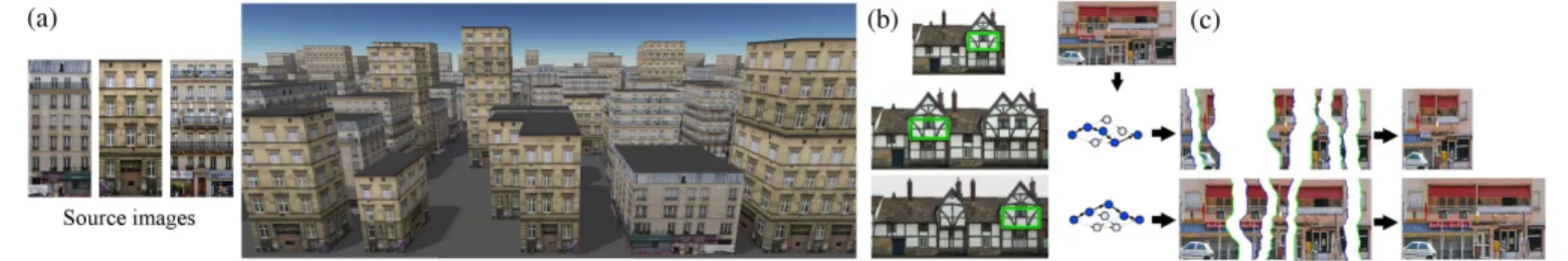
Figure 1: (a) From a source image our synthesizer generates new textures fitting surfaces of any size. (b) The user has precise control over the results. (c) Our algorithm synthesizes textures by reordering strips of the source image. Each result is a path in a graph describing the space of synthesizable images. Only the path need to be stored in memory. Decoding is performed during display, in the pixel shader.
Abstract
Textures are often reused on different surfaces in large virtual envi-ronments. This leads to unpleasing stretch and cropping of features when textures contain architectural elements. Existing retargeting methods could adapt each texture to the size of their support sur-face, but this would imply storing a different image for each and every surface, saturating memory. Our new texture synthesis ap-proach casts synthesis as a shortest path problem in a graph de-scribing the space of images that can be synthesized. Each path in the graph describes how to form a new image by cutting strips of the source image and reassembling them in a different order. Only the paths describing the result need to be stored in memory: synthesized textures are reconstructed at rendering time. The user can control repetition of features, and may specify positional con-straints. We demonstrate our approach on a variety of textures, from facades for large city rendering to structured textures commonly used in video games.
1
Introduction
Textures are an essential primitive of Computer Graphics. They are responsible for most of the detail we perceive in computer gen-erated images. In this paper, we focus on textures applied to ur-ban scenery and buildings. These textures often contain a mix of materials—concrete, bricks, stones—and structure—windows, doors, lanes, control panels. We refer to such textures as architec-tural textures.
A typical difficulty is that architectural textures are created with a given surface size in mind. For instance, facade textures captured from photographs will only apply to buildings of the appropriate size. Door images will only apply to the corresponding door panels. Enlarging or changing the size of the surfaces results in a stretched, unpleasing and unrealistic appearance. In addition, it is often not possible to customize every texture to every surface. A first issue is of course limited authoring resources. A second, major issue comes from the extremely large quantity of data that would result from
having a unique texture per surface. In the context of interactive applications the cost of such a large database of textures both in terms of storage and rendering complexity is prohibitive.
Our approach addresses both issues at once: It synthesizes, from an example, new textures fitting exactly the support surfaces and stores the result in a very compact form, typically just a few kilo-bytes. Results are directly used under their compact form during rendering. Decoding is simple enough to fit in a pixel shader. Us-ing our technique, modelers only have to prepare a limited database of high quality textures: a new, unique texture resembling the orig-inal is synthesized for each surface, typically in less than a second. If the user is not satisfied with the result, several interactive controls are possible, such as explicit feature positioning through drag-and-drop. This all comes at a small cost since results are compactly stored during display, and efficiently rendered.
To achieve this, we exploit specificities of architectural textures. Our assumption is that the textures tend to be auto-similar when translated along the main axes. This is easily verified on architec-tural textures. However our approach only applies to this subclass of images, and will be less efficient on arbitrary images. The tech-nique is fully automatic, unless the user wants to achieve a particu-lar goal, such as putting a door or window at a given location. We use the self-similarities in the textures to define a generative model of the image content. In that sense, each image is turned into an image synthesizer able to generate visually similar images of any size. Once constructed, the synthesizer quickly generates textures of any width and height and outputs the result in a compact form. The synthesizer proceeds successively in vertical and hor-izontal directions, the second step using the intermediate result as the source image. In each direction, it
syn-thesizes a new image by cutting horizontal (resp. ver-tical) strips of the source image and pasting them side by side in a different order. This is illustrated along the x direction Figure 1 (c). We search the source image for repeated content in the form of horizon-tal (resp. vertical) parallel paths along which similar colors are observed. Two such parallel paths are indi-cated by the green/blue triangles in the inset. We call these paths cuts as they define the boundaries of the strips that we “cut out” from the source image. We
extract many such parallel cuts from each source image. Any pair of non-crossing cuts defines a strip, and the strips can be assembled with a number of other strips like in a puzzle (Figure 1 (c)). The par-allel cuts create many choices in the way strips may be assembled.
This is the source of variety in the synthesized textures. Intuitively, given a target size our algorithm automatically determines the best choice of strips to both reach the desired size and minimize color differences along their boundaries. Despite the apparent combina-torial complexity of the problem, given a set of cuts we are able to solve efficiently for it using a graph-based formulation. The opti-mization reduces to a simple shortest-path computation. The solu-tion path describes the sequence of cuts that form the boundaries of each strip; it is thus very compact.
Our contributions are:
• The formulation of the unidirectional architectural texture synthesis problem as a graph path-finding problem, together with a construction algorithm for finding cuts and building the graph for a given image (Section 3),
• An algorithm to quickly generate an image of any desired width and height, using two successive unidirectional syn-thesis steps (Section 4), possibly enforcing some constraints for higher visual quality or user-control over the result (Sec-tion 5).
• A compact encoding of synthesized textures in GPU mem-ory, together with a simple algorithm to sample them from the pixel shader (Section 6).
Applications range from large virtual city rendering to adapting structured textures to their support surfaces in video game environ-ments (Section 7).
2
Previous work
Generating rich and detailed textures for virtual environments is a long standing goal of computer graphics. We present here the works most related to synthesis of architectural (structured) textures.
Procedural architectural textures A first approach to adapt tex-tures to surfaces and reduce authoring time is to procedurally gener-ate the textures. Early approaches for structured textures are based on cellular noise [Worley 1996]. Lefebvre and Poulin [2000] pro-pose to learn the parameters from existing images for specific ma-terials. M¨uller et al. [2007] fit a grammar on photographs of fa-cades to deduce a generative model of their geometry. We compare this approach to ours for the specific case of facades in Section 7. Legakis et al. [2001] generate complex structured layouts of bricks and stones on the walls of buildings.
Content synthesis from example Example-based texture syn-thesis methods [Wei et al. 2009] generate new textures of any size resembling a small input image. Most of these methods focus on textures of unstructured, homogeneous aspect and require to pre-compute and store the resulting images. The approach of Sun et al. [2005] fills holes in structured images by pasting overlapping patches at discrete locations along user defined curves, minimizing for color differences. Sch¨odl et al. [2000] synthesize infinite video loops by cutting and re-ordering pieces of an example sequence. Loops are formed by jumping backward in time to matching frames. This could be applied to images, jumping from one column to an-other. Compared to this scheme our graph formulation allows for arbitrarily shaped cuts and is not limited to backward jumps.
Image retargeting and reshuffling Recently, a new set of tech-niques have been developed to retarget images for displays of var-ious sizes. While not exactly our goal, this could be used to adapt textures. Several approaches deform a mesh overlaid on the im-age, focusing stretch in areas where it is less noticeable [Gal et al.
2006; Wang et al. 2008; Cabral et al. 2009]. Instead, the seam carv-ing approach [Avidan and Shamir 2007] iteratively removes rows and columns having low gradient in the image, one at a time. Ru-binstein et al. [2009] extend the approach to compromise between stretch, crop, and seam carving.
These early methods strive to preserve all the content initially in the image. Instead, the approach of Simakov et al. [2008] summarizes the image content, discarding repetitive information. An interest-ing new application suggested in this work is the reshufflinterest-ing of the image content, giving the ability to change the layout of features in the image. Recent approaches formulate reshuffling as a labeling problem, either at the patch level [Cho et al. 2008] or at the pixel level [Pritch et al. 2009]. These approaches are generally slow since they are iterative and based on patch matching; however they can be brought to interactivity using stochastic patch search [Barnes et al. 2009]. In all cases, the output is a new image that must be stored, hindering their use for textures in large environments.
Our goal is to provide similar functionalities for architectural tex-tures, while affording compact storage of the result. Our proach draws inspiration from patch-based texture synthesis ap-proaches [Kwatra et al. 2003]—we reorder pieces of the source image—and seam carving [Avidan and Shamir 2007]—we work successively with horizontal or vertical strips of the initial image. However, by relying on a graph–formulation for the choice of strips we quickly obtain results of very high quality—the best possible for the given set of cuts—and easily account for global constraints, en-abling user controls. In addition, only the paths need to be recorded in memory, resulting in a very compact encoding of the results.
3
Unidirectional synthesis
3.1 Overview
Given a source image, our approach first prepares a synthesizer in a preprocessing step. The synthesizer is then used to produce visually similar images of any size. The output is a compact data structure directly used by the renderer to texture 3D models.
The image synthesizer operates in a single direction at a time, hor-izontally or vertically. Hence, two successive synthesis steps are necessary in order to generate images of given width and height. In the following we discuss unidirectional synthesis only, and later focus on bidirectional synthesis in Section 4. For simplicity, we describe synthesis in the horizontal direction.
In order to build a horizontal synthesizer, we first search the im-age for parallel vertical cuts (Section 3.4), and then build a directed graph (digraph) representing the space of all images that can be syn-thesized (Section 3.2). We describe first the digraph construction and synthesis step since they constitute the heart of our approach. We introduce below the definitions used throughout the paper.
Pixels We note[N ] the integer interval [0..N − 1]. The source image has width W and height H. The lower left pixel has coordi-nates(0, 0).
Cuts A vertical cut c is a function[H] 7→ {−1} ∪ [W ] such that|c(y) − c(y + 1)| ≤ 1 for all y ∈ [H]. We understand c as a cut between the pixels in the image: for all y in[H] we cut the image vertically along the right boundary of pixel(c(y), y) so as to separate the image in two pieces. For any cut c, we define cmin=
miny∈[H]c(y), cmax= maxy∈[H]c(y) and the width ω(c, c′)
between cuts c and c′as ω(c, c′) = c′
min−cmin. Similar definitions
Partial order on the cuts LetC denote a set of cuts. We define a partial order onC as follows. Given two cuts c and c′, we say that c precedes c′ if and only if c 6= c′ and for all y ∈ [H] we have c(y) ≤ c′(y). We write precedence as c ≺ c′. Two distinct cuts c and c′crosseach other if none precedes the other.
Given a cut c (shown yellow in-set) we define the successors of c as Succ(C, c) = {c′ ∈ C | c≺ c′}
(shades of green and blue inset). We say that c ∈ C is a front cut of C if it has no predecessor inC. We write Front(C) the set of front cuts of C (we show insetFront(Succ(C, c)) in shades of green). Note that the cuts inFront(C) are pairwise crossing.
Parallels Two cuts c and c′are parallel iff c′(y)−c(y) = ω(c, c′)
for all y∈ [H]. A cut is parallel to itself. Let P(c) denote the set of cuts inC that are parallel to c. Two parallel cuts are illustrated in the inset picture on the first page bottom.
Costs Each pair of parallel cuts(c, ck) is associated with a cost
δ(c, ck). In our implementation, this cost is the sum of the color
differences along the cuts, raised to a power p (we use p= 4): δ(c, ck) =
X
y∈[H]
||I(c(y) + 1, y) − I(ck(y) + 1, y)|| p
where I(x, y) is the pixel value at x, y in the image. Increasing p penalizes cuts that match well overall but have a few large mis-matches. Note that δ(c, c) = 0.
3.2 Assembling strips
We now describe our formulation for unidirectional synthesis. We define an assembly of strips from the source image as a sequence of cuts A= c⋆, c0, c0
k, ..., c n, cn
k, c†where c ⋆
, c†are starting and ending cuts chosen by the user (typically the first and last columns of the source image), and ci, ci
kare the ending and starting cuts of
two successive strips (see Figure 2). Since they must have the same shape these two cuts are parallels: cik∈ P(ci)\{ci}. The assembly
quality depends on how well colors along the cuts are matching. We define the assembly cost as: δ(A) =Pni=0δ(ci, ci
k).
Let ω(A) be the width of the image resulting from the assembly A. We are searching for an assembly Abest minimizing δ while
producing an image of desired target widthT , i.e.: Abest= argmin
A st. ω(A)=T
(δ(A)).
We optimize for the best possible assembly by turning the problem into a simple shortest path search in a directed graph. (We only consider directed graphs, so we will use the shorter term “graph”.)
Generative graph Our reasoning for the graph formulation is as follows: Consider we add cuts—rather than strips—to the image under construction, one at a time from left to right. At any given time the partially grown image ends with a cut c. From this cut we are given two choices on how to continue (see Figure 2):
1. Grow the rightmost strip by adding to the image one of the cut c′ located after c in the source, that is a cut in Succ(C, c). In this case, we limit the choice for c′ to cuts
in F(c) = Front(Succ(C, c)) without loss of generality since a cut c′ ∈ Succ(C, c) is either in F(c) or is separated from c
by at least one cut in F(c). This restriction on the choices for c′reduces the number of edges in the graph to be described below, roughly, from O(|C|2) to O(|C|).
2. Start a new strip by jumping to a cut parallel to c, that is a cut inP(c) \ {c}. This strip may be later grown.
In the first case we enlarge the image by ω(c, c′) and add no error
to the assembly. In the second case we do not enlarge the image but add an error δ(c, ck) to the assembly cost.
Figure 2: Left: Cuts are added one by one to the image from left to right, eithergrowing the current strip by adding a cut (green), or starting a new strip by jumping from a cut to its parallel counterpart (red).Right: The end result, formed of six strips from the source. We model these choices as a graph G= (C × Z, E≺⊔ Ek) where
⊔ is the disjoint union. Each node (c, z) ∈ C × Z represents the cut c translated to abscissa z in the result image. More precisely, the translated cut is located in the result image at(c(y) − cmin+ z, y)
for all y∈ [H]. Thus, while the cuts are defined in the source im-age, the nodes of the graph are defined in the result image. The growth edges E≺and the start edges Ekcapture the choices
dis-cussed above and are defined as:
E≺ = {(c, z) → (c′, z+ ω(c, c′)) | (1)
c′∈ Front(Succ(C, c)), z ∈ Z}
Ek = {(c, z) → (c′, z) | c′∈ P(c) \ {c}, z ∈ Z} (2)
Intuitively, edges in E≺tell us that if we depart from a cut c
lo-cated at z in the result image and grow the strip until a cut c′ ∈ Front(Succ(S, c)), then the next cut c′is located at z+ ω(c, c′).
Edges in Eksimply replace the current cut by its parallel
counter-part, without changing the current location. The cost of each edge((c, z), (c′, z′)) ∈ E
kis set to δ(c, c′) and
edges in E≺are given a null cost.
Paths as images We specify the start and end of the result image with two cuts c⋆and c†. These two cuts are typically located at the left and right border of the source image but could be any other pair of cuts, possibly chosen by the user. Refer to Section 5 for more details on user controls.
Finding the best assembly for an image of size T thus simply amounts to finding a path in G from node(c⋆, c⋆
min − c⋆max) to
node(c†,T ) since the assembly of strips corresponding to such a path does contain a rectangle of widthT . We use Dijkstra’s algo-rithm to globally minimize the cost of the resulting assembly. The graph G is infinite, but for a desired widthT we need only con-sider a finite subgraph G′ = (C × [c⋆
min− c⋆max..T ], E≺⊔ Ek),
because the z component of the nodes along any path in G form a non-decreasing sequence.
Graph traversal For space efficiency during Dijkstra’s algorithm execution, we generate the graph edges implicitly from its nodes: growth edges are generated from the setsFront(Succ(C, c)) that we keep in memory for each cut c∈ C (see Eq. 1). Similarly, start
Figure 3: Enlarging from 512 to 600 pixels with ξ = 600. Left: Without threshold (R = ∞), the chimney appears ten times in a row.Right: With a threshold R= 4, the result is visually improved.
edges exiting a node(c, z) are deduced by storing with c a pointer to its set of parallel cuts (see Eq. 2).
3.3 Limiting repetitions
Our graph formulation above works well as such for synthesizing images of width smaller than the source. However, for larger im-ages undesirable repetitions appear: in the result image, two nodes with the same cut appear repetitively at successive nearby locations (see Figure 3).
We implement a histogram-based scheme to avoid such behavior. It takes two parameters: a window size ξ ∈ N and a threshold R ∈ N⋆. We search a path in G constrained so that in any crop of full-height and width ξ of its corresponding output image, no column of the source image is repeated more than R times. Since most cuts are not vertical, a column in the result is not necessarily a column from the source image. We thus consider, as an approximation, that following a growth-edge((c, z), (c′, z′)) copies the source columns with index in(cmin, c′min] into the result. In Dijkstra’s algorithm we
do not follow an edge if it would result in a path not enforcing the constraint. An example of limiting repetitions is given in Figure 3. This limitation scheme is enabled by default in our implementation and all the results in the paper use ξ = 100 and R = 2, except where otherwise stated.
3.4 Finding parallel cuts
The construction of the set of cutsC is a crucial step for our tech-nique. First, in terms of quality since we want parallel cuts with minimal cost. Second, in terms of performance since a larger num-ber of cuts makes the graph larger and longer to build, and slows down the shortest paths search.
A cut inC that has no corresponding parallel cut is useless for our purpose, since it does not introduce new possible assemblies. We thus search for pairs of parallel cuts(c, ck) to be inserted in C. Two
main criteria guide us in our search for pairs. First, parallel cuts with a large cost are wasteful since the start-edges joining them will most often not be followed, and if followed would result in a noticeable mismatch. Second, we want to avoid an accumulation of low-cost parallel cuts in a same area of the image as this results in a large number of similar paths having similar costs. This increases the size of the graph significantly with no benefit. On the contrary, pairs of a given width should cover as much of the source image as possible. This variety helps the method finding paths even in con-strained cases, for instance when user control is used (Section 5). For finding parallel cuts, we use the procedure given in pseudocode hereafter. In line 1, we use EσI(x, y) = ||I(x, y) − I(x + σ, y)||
p
. In line 2, π is the minimal-cost Y -monotone path from the top to the bottom row of EIσ; it is computed using dynamic programming
just as in [Efros and Freeman 2001]. In line 3, the two parallel cuts (c, ck) satisfy ω(c, ck) = σ and their cost δ(c, ck) is that of the
path π. Line 4 is the heuristic that we use to enforce that all the pairs of width σ be well spread over the image while not being too
Figure 4: From left to right: Parallel cuts obtained for width σ= 5, 11, 19 and 58. Each blue cut has a parallel green counterpart.
numerous (Figure 4). On a source image of size2562, for example,
the procedure typically finds around 600 pairs, with at least the best pair for each width.
for width σ from1 to W − 1 do
1 Compute an error map EσI of size[W − σ] × [H].
2 while the shortest-path π from top to bottom of EIσhas finite cost do 3 Augment C with the two parallel cuts corresponding to π. 4 In Eσ
I, set the value of pixels less than σ pixels away from π to ∞.
The preprocessing stage for one source image consists in computing a set of vertical cuts for horizontal resizing and a set of horizontal cuts for vertical resizing. These sets are stored on disk for later use.
4
Bidirectional synthesis
We described previously how to synthesize new images of arbitrary width or height. In most scenarios, however, a bidirectional syn-thesis is required. We rely on the fact that our synthesizer directly generates images of the desired width in one step: We apply two successive synthesis operations, one in each direction. The second synthesis step uses the intermediate result as a source image. This fits well with our goal of compactly encoding results in GPU mem-ory, as only one vertical and one horizontal assembly are stored for each result. While the two possible orders of synthesis steps may produce different results, we observe that they are often very simi-lar. All the results in this paper are obtained using vertical followed by horizontal synthesis.
After the first, vertical synthesis step, the vertical cuts for the hori-zontal synthesis have to be computed on the intermediate result. We provide a fast way to do so, as explained in Section 4.1. The graph for horizontal synthesis is then computed, and the second synthesis step proceeds. Section 4.2 explains how to accelerate the synthesis of many images of different sizes from a single source image.
4.1 Fast cut update
During bidirectional synthesis the computation of new cuts on the intermediate result becomes a bottleneck when synthesizing a large number of images. We propose an approximate but very fast way to obtain the cuts. We assume in the following vertical followed by horizontal synthesis. We discuss computation of vertical cuts for the second, horizontal synthesis step.
We observe that the vertical cuts computed as in Section 3.4 in the intermediate result tend to be locally identical to the vertical cuts in the source image. For instance, compare Figure 5 (b) and (d). We exploit this property to quickly compute new cuts. During the initial cut computation in the source image, we record for each width σ a path map PIσin memory. It has the same size as the error map E
σ I.
Each entry PIσ(x, y) is in {−1, 0, 1} and indicates to which pixel
to continue to reach the top of the error map with minimal cost. PIσ
is initialized using dynamic programming on the error map prior to the first path extraction (Section 3.4). After all vertical paths have been extracted we update PIσas follows: each pixel in PIσalong a
(a) (b) (c) (d) Figure 5: Only parallel cuts of width σ= 24 are shown for clarity. From left to right: (a) Source image, (b) precomputed parallel cuts for horizontal synthesis, (c) fast update of the vertical cuts; the cuts used for vertical synthesis are shown in red, (d) parallels obtained with exact computation on the intermediate result. The cuts in (c) and (d) are very similar.
path is updated with the direction of that path at that position. We finally record the starting abscissa of each path. Thus, following PIσ
from these abscissa will reconstruct the same paths. Starting from any other location in PIσrapidly leads back to one of the paths.
The first, vertical synthesis step produces an assembly Avof
hori-zontal strips from the source image. We apply Avto the path map—
cutting it instead of the source image—to obtain a new path map P′ corresponding to the intermediate image. Since the path map is nar-rower by σ pixels than the source, we crop the cuts of Avto width
W − σ. We then follow the directions given by P′, starting from
the recorded abscissa, to construct new paths from which we de-duce pairs of parallel cuts just as in Section 3.4 (Figure 5 (c)). We finally compute the cost of each pair using the intermediate result. This process produces a new set of parallels in tens of milliseconds for all widths σ. It is approximate however, so there is no guaran-tee that the new paths are of minimal-cost in the error map of the intermediate result. However, since the cost of each new pair of parallel cuts is recomputed, bad pairs will tend to be avoided when traversing the graph G. Figure 5 compares the fast cut update to the computation described in Section 3.4.
4.2 Synthesizing in bulk
Our goal is to generate, from a source image, a unique texture for many different surfaces. A good example of this scenario is the vir-tual city described in Section 7, where a small set of facade textures are customized to fit every facade of every building.
In this situation, we benefit from the fact that Dijkstra’s algorithm computes a one-to-all shortest-paths tree: The vertical synthesis steps of all images start from the same node in G (typically the top row of the source image). There are of course multiple end nodes, corresponding to the various requested heights. By keep-ing in memory the shortest-paths tree between successive calls to the Dijkstra’s algorithm, we benefit from the previously computed shortest-paths. However, this cannot be done for the second synthe-sis step unless intermediate results are the same (i.e. same height, different widths). Nevertheless a significant speedup is achieved. For example, generating 10 images of height 588 and width ranging from 200 to 2000 takes 24.2 seconds in total if Dijkstra’s algorithm is restarted from scratch for each image. Using our scheme, it takes 5.9 seconds to generate all the images.
5
User control
Our algorithm may operate automatically, but also provides several user controls over the synthesized images. In particular, the user
may require some features to appear no more than a given number of times (Section 3.3), to be precisely localized (Section 5.1), or may want a variety of results of a same size (Section 5.2). We focus below on the later two forms of control.
5.1 Explicit feature positioning
Explicit positioning lets the user specify where features of the source image should appear in the result. This is a convenient control for architectural textures. We discuss below two possible approaches: The first, simple and fast, lets the user directly manip-ulate cuts in the result. However, choosing the right cuts to position features may be difficult. The second, more elaborate, provides an accurate drag-and-drop control.
Splitting the path Using this simple control, the user explicitly specifies a set of control nodes in the graph G that should be part of the output path. The control nodes are sorted and included in between the initial start and end nodes. Then, a shortest path is computed between each pair of consecutive nodes.
This approach has the advantage of simplicity, but the result strongly depends on which cuts are manipulated. Nevertheless, this control mechanism has proven useful in our experiments: visually good results are consistently achieved, and moving a control node around (i.e., changing(c, z) to (c, z′)) is fast since the shortest-paths trees generated with Dijkstra’s algorithm are kept in memory (Section 4.2). Figure 7-bottom illustrates this type of control.
Drag-and-drop control Here, we seek a path of minimal cost in G, such that a region specified in the source appears at a desired location in the output. The user selects a source regionRs
sand-wiched between two special cuts m and M subject to
m(y) ≤ M (y) and (m(y) = ∞ ⇔ M (y) = ∞) for all y ∈ [Y ]. The user then specifies the abscissa∆ ∈ Z where the region must be located in the output: Pixel colors at position{(x, y), m(y) 6= ∞ and m(y) < x ≤ M (y)} in the source should appear at position (x+∆−mmin, y) in the synthesized image. Those target positions
together form the target regionRt.
We note X the (possibly empty) set of nodes whose cut intersects Rtin the result, L the set of nodes to the left ofRt(≺ m), and R
the nodes to the right (≻ M ). Assuming L and R are non empty, a satisfying path always starts with a node in L and ends in R. In addition, it can only transition through X (L→ X, X → X, X→ R) or from L to R via edges between well aligned nodes, that is nodes(c, z) with z = cmin+ ∆. This ensures that Rtcontains
the properly aligned selected part of the image. If L (resp. R) is empty the starting (resp. ending) node belongs to X. In Dijkstra’s algorithm loop, we discard edges that do not obey the above rules. The set of integers z for which(c, z) ∈ X is an interval since Rt
is Y -monotone. We store these intervals to check in constant time if an edge can be followed or not. This easily extends to multiple control regions. Figure 1 (b) shows results obtained in this way.
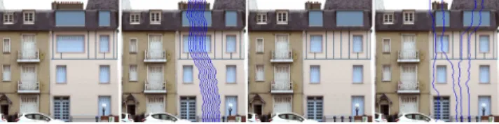
5.2 Introducing variety
By default, our algorithm always generates the same image for given target size, histogram and user-control parameters. We im-plement an optional mechanism to automatically introduce variety as we successively synthesize new images from the same set of pa-rameters. Let Cji be the column of the source image that appears
as the j-th column in the i-th result image (we make the same ap-proximation as in Section 3.3). Successively synthesized images
are forced to be different by ensuring that for all j, Cij is farther
than D pixels away from Cij′ for all i
′ < i. That constraint is
ig-nored for values of j closer than2 × D pixels from the result image boundaries, since all results start and end similarly. We implement the constraint in Dijkstra’s algorithm by ignoring edges which, if followed, would put two columns closer than allowed. Refer to Figure 8 (top) for results.
6
Rendering
We now describe how synthesized textures are applied to surfaces, having only the source image(s) and the assemblies describing the results in GPU memory. The result images are reconstructed on-the-fly, with proper filtering, in the pixel shader: we focus on ren-dering with a programmable GPU for real-time applications, but the technique applies equally well to off-line rendering.
Data structure In order to reconstruct a single result we only need to store the horizontal and vertical paths. Multiple results pro-vide further opportunities for memory savings: Many of the pre-computed cuts used in the first, vertical synthesis step are likely to appear in more than one result. However, the cuts generated for horizontal synthesis cannot generally be shared.
On the GPU we store all the cuts, vertical and horizontal, in a sin-gle 2D texture: the cut table. Since they correspond to different results, they have different lengths. We pack them together while heuristically minimizing wasted texture space. Each result is then encoded in two arrays, one for each path. For each node(c, z) in a path we store in the array the index of the cut in the cut table, and its location z in the result. Each pair of consecutive entries in the array defines a strip of the assembly.
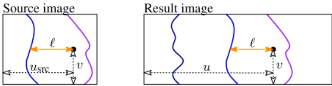
Sampling and filtering During rendering, a small program—the pixel shader—is executed by the GPU at every pixel to determine its color. Each pixel is associated with a texture coordinate u, v. With standard texturing the texture image stored in memory is sampled at the u, v location to obtain the pixel color.
Our goal is to find the color of each pixel using only the cuts, with-out ever having to decode the entire result image in memory. In each pixel we thus must find the coordinates usrc, vsrcin the source
image corresponding to the texture coordinate u, v in the result. When performing a bidirectional synthesis, it is easy to see that the horizontal (resp. vertical) step changes only the x (resp. y) coordi-nate of the pixel. Computations on u and v must be performed in the reverse order of synthesis to take into account the intermediate result: We obtain usrcfrom u, v and then vsrcfrom usrc, v. In a given
direction, we first locate the strip enclosing the lookup coordinate in the result. We perform a binary search using the positions of the cuts. From there, we easily locate the source coordinates using the left strip border (see illustration hereafter).
ℓ
u ℓ usrc
Source image Result image
v v
A key issue when rendering from a pixel shader is to ensure the result is filtered: the texture must be smoothly interpolated at close-ups and properly blurred when seen at a distance (typically using MIP-mapping). The GPU filtering mechanism breaks around cuts since it is unaware of the discontinuities: visible seams appear. One approach would be to re-implement the trilinear interpolation
mechanism. However, while feasible, this would be slow and would not support anisotropic filtering which is an important feature when rendering flat surfaces such as walls and facades. Instead, we blend the filtered lookups from both sides of a cut, hiding the interpola-tion seams. The blending weights are computed as a funcinterpola-tion of the distance to the cut and the filtering level. We treat both directions separately to enable support for anisotropic filtering. This removes all visible artifacts, even though discontinuities still exist at very coarse magnification levels where blending should involve multiple strips (please refer to the supplemental material).
7
Applications and results
We now present results and timings. All results are obtained on an Intel Xeon E5520 2.3 GHz using a single core for computations. The GPU is a NVidia Quadro FX 3800.
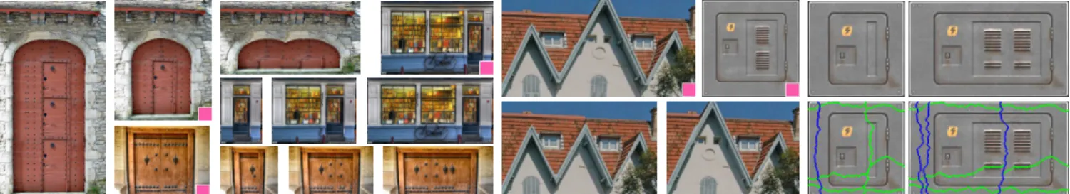
Synthesis of architectural textures We tested our approach on a number of architectural textures: floors, doors and window frames, fences and even structured photographs. The only parame-ter we change for these results is the number of allowed repetitions. We typically require no more than two repetitions in any crop a hundred pixels wide (ξ= 100 and R = 2).
Figure 6 and 7 show a number of results, from simple ones to chal-lenging cases. Table 1 gives timings for some of these images, in-cluding preprocessing for searching cuts—performed only once for a source image— and timings for synthesizing a new image. For each result image, we distinguish timings of each synthesis step and indicate how long the cut and graph update took. Note these are timings for the first result, when no shortest path has been pre-viously computed. Subsequent results are faster to synthesize. Result quality is overall very good, with very few visible disconti-nuities. Note that some remaining visible cuts in our results could be easily avoided by working in the gradient domain. However, this would impede compact encoding on the GPU.
Controlled Synthesis The user can directly specify where parts of the image should appear. This is illustrated Figures 1 (b) and 7 as well as in the accompanying video. Explicit positioning adds very little cost: precomputing the intervals for the drag-and-drop control takes 5 to 6 milliseconds, and the predicate that decides if an edge can be followed or not adds a negligible cost to the synthesis time.
City modeling The city modeling application reveals the key ad-vantage of our approach compared to standard image resizing tech-niques. Since each synthesis result is compactly encoded, we are able to customize a facade texture to each and every surface of an entire city. Figure 1 shows a city with 7488 facades (1672 build-ings), using 13 different texture images as sources (9.9 MB). Stor-ing a texture for each facade would require 6.9 GB of GPU memory. Instead, using our scheme, each facade gets a unique texture and all facades occupy 60 MB of GPU memory (excluding the source images); two orders of magnitude less. The textures are decoded in every pixel, from the pixel shader. The entire city renders at 195 FPS on average at1600 × 1200 resolution, without deferred shading or visibility culling. All computations for the facades took
Source Preproc. Synth.= V synth. + Cuts + Graph + H synth. Fig. 6 right (256x256) 2.5 0.8 0.06 0.02 0.19 0.5 Fig. 7–A(340x512) 20.3 5 3 0.1 0.9 1 Fig. 7–B(512x512) 22.7 6.7 1 0.16 2.3 3.2 Fig. 7–C(512x349) 21.8 5.4 0.88 0.1 2 2.4
Figure 6: Various syntheses. Sources are marked with a pink square. Right: Source is slightly downscaled, bottom results have cuts overlaid. 78 minutes, for an average of 625 ms and 8 KB per facade. As can
be seen on these images as well as on the accompanying video, fil-tering is well behaved, showing no artifact even at grazing angles. Anisotropic filtering is enabled in all renderings.
Comparison to grammar-based facade synthesis The ap-proach of [M¨uller et al. 2007] fits a grammar on a facade image, enabling procedural generation of new facades. It operates at the se-mantic level, explicitly detecting rectangular shaped windows and doors. In contrast, our approach operates at a lower level and does not require a description of the image content. A drawback is that it may produce semantically improper results such as narrow or asym-metric doors or windows. However, it applies in a larger number of cases such as decorated, complex, partially occluded or unusual facades (see Figures 6 and 7). Our approach complements well grammar-based techniques, providing a good alternative when the grammar cannot interpret the image content.
Variety Figure 8 (top) shows an example of introducing variety using our algorithm. Four successive results of size equal to the source are synthesized. The leftmost image—the first result—is exactly similar to the source. All three successive images are con-strained to be different from the previous ones.
Comparison to retargeting Our approach synthesizes a variety of images of different sizes resembling the input, while retargeting generates images preserving all the content visible in the original. In Figure 8 (bottom) we compare our approach with that of Avidan and Shamir [2007] and Simakov et al. [2008] for enlargement. On the more elaborate scheme of Simakov et al. results are very simi-lar. However we have the possibility to quickly generate a variety of new, different images. In addition, the result of retargeting ap-proaches are new images which cannot be compactly stored during rendering. Of course, latest retargeting approaches do not require our strong assumption about the content, and there are many images we could not deal with.
Limitations The main limitation of our approach is that it focuses on architectural textures, expecting repetitions to occur mostly along the x and y directions. Figure 9 shows two failure cases. In both, either no repetition exist or the repetitions are not aligned with the main axes producing artifacts in the results. As mentioned earlier, our method has no semantic information and may produce unrealistic features (such as narrow doors, long cars).
Another limitation is that a path may not always exist when pforming user control, or the path found may have a very large er-ror. Using arbitrarily shaped curves rather than Y -monotone curves would add more freedom and allow for more complex behaviors. The graph formulation does not have to be changed, but this com-plicates storing and decoding the cuts in the GPU. We leave this issue for future work.
Finally, on extreme enlargements large scale repetitions may
ap-Seam carving
Ours
[Simakov et al. 2008]
Figure 8: Top row: Four results of same size with variety. (D= 48, R = 3, ξ = ∞). Bottom: Comparison with retargeting.
Figure 9: Left pair: Source image [Barnes et al. 2009], our result. Right pair: source without vertical repetition, our result.
pear, producing a distracting tiling effect. As future work, we plan to implement a mechanism similar to the one for variety but within a same image, so as to avoid these large scale repetitions.
Conclusion
Our approach significantly reduces authoring time of large environ-ments while preserving rendering performance, both in time and memory consumption. Each support surface is fitted with a texture of the correct size and aspect-ratio, thereby improving the overall visual quality. The technique appears robust and fast enough to be used as an interactive and creative tool for the transformation of texture assets in virtual worlds.
We believe the graph based formulation of our approach is espe-cially well-suited for synthesizing structured content decomposed in basic blocks, while enforcing non trivial user constraints. In par-ticular, it is easy to generalize the formulation to any other type of content as long as synthesis can be decomposed in a set of succes-sive unidirectional operations (not necessarily axis aligned or along a straight line). We hope this will spark further research in the field of by-example content synthesis.
Acknowledgments and Credits We thank Laurent Alonso, George Drettakis, Bruno L´evy, Nicolas Ray and Rhaleb Zayer for proof–reading the paper. Credits for the source images go to: Claire Royer (Figure 7,top right), Asmodai Tabun (video game textures, Figures 6, 7, 9), Denyse Schwab (Mandala, Figure 7), Yaron Caspi (Jerusalem, Figure 8), Flickr users
Sev-A
B
C
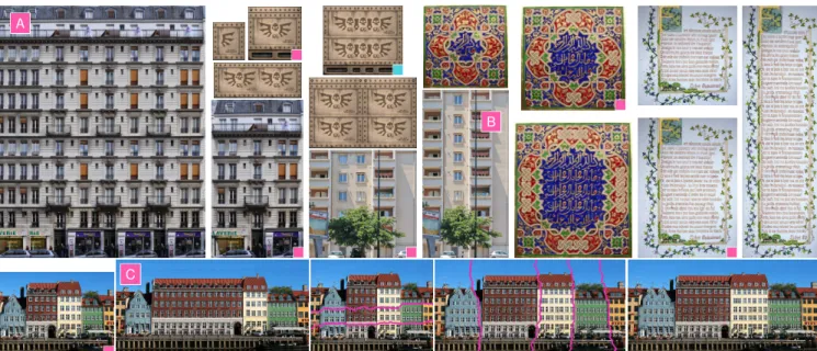
Figure 7: Top: Synthesis results. Source images are marked with a pink square. The histogram window size parameter ξ is250 for the leftmost image. Drag-and-drop control is used on the image marked with a blue square. Bottom, left to right: The Copenhagen harbor. Automatic enlargement. 2 control cuts (in pink) to add one floor. 4 control cuts to set the building sizes. Final result.
enbrane(greek temple, Figure 9), Dynamosquito (doors, Figure 6), Bcn-bits(bookstore, Figure 6), www.cgtextures.com (Figure 1 (a (middle), b), 3, 4, 5), [Teboul et al. 2010] (Figure 1 (a (left, right)), Figure 7A),
Cen-tre Scientifique et Technique du Bˆatiment (all other facades). This work was funded by the Agence Nationale de la Recherche (SIMILAR-CITIES ANR-2008-COORD-021-01) and the European Research Council (GOOD-SHAPE FP7-ERC-StG-205693).
References
AVIDAN, S.,ANDSHAMIR, A. 2007. Seam carving for content-aware image resizing. ACM Transactions on Graphics (Proc. ACM SIGGRAPH) 26, 3.
BARNES, C., SHECHTMAN, E., FINKELSTEIN, A.,ANDGOLD
-MAN, D. B. 2009. PatchMatch: A randomized correspondence algorithm for structural image editing. ACM Transactions on Graphics (Proc. ACM SIGGRAPH) 28, 3.
CABRAL, M., LEFEBVRE, S., DACHSBACHER, C.,ANDDRET
-TAKIS, G. 2009. Structure preserving reshape for textured archi-tectural scenes. Computer Graphics Forum (Proc. Eurographics conference) 28, 2.
CHO, T. S., BUTMAN, M., AVIDAN, S.,ANDFREEMAN, W. T. 2008. The patch transform and its applications to image edit-ing. In Proc. IEEE Conference on Computer Vision and Pattern Recognition (CVPR).
EFROS, A. A.,ANDFREEMAN, W. T. 2001. Image quilting for texture synthesis and transfer. In Proc. ACM SIGGRAPH, 341– 346.
GAL, R., SORKINE, O., AND COHEN-OR, D. 2006. Feature-aware texturing. In Rendering Techniques, Proc. Eurographics Symposium on Rendering, 297–303.
KWATRA, V., SCHODL¨ , A., ESSA, I., TURK, G.,ANDBOBICK, A. 2003. Graphcut textures: Image and video synthesis using graph cuts. ACM Transactions on Graphics (Proc. ACM SIG-GRAPH) 22, 3.
LEFEBVRE, L.,ANDPOULIN, P. 2000. Analysis and synthesis of structural textures. In Proc. Graphics Interface (GI), 77–86. LEGAKIS, J., DORSEY, J., ANDGORTLER, S. 2001.
Feature-based cellular texturing for architectural models. In Proc. ACM SIGGRAPH, 309–316.
M ¨ULLER, P., ZENG, G., WONKA, P.,ANDGOOL, L. V. 2007. Image-based procedural modeling of facades. ACM Transactions on Graphics (Proc. ACM SIGGRAPH) 26, 3.
PRITCH, Y., KAV-VENAKI, E., ANDPELEG, S. 2009. Shift-map image editing. In Proc. IEEE International Conference on Computer Vision (ICCV).
RUBINSTEIN, M., SHAMIR, A.,ANDAVIDAN, S. 2009. Multi-operator media retargeting. ACM Transactions on Graphics (Proc. ACM SIGGRAPH) 28, 3.
SCHODL¨ , A., SZELISKI, R., SALESIN, D.,ANDESSA, I. 2000. Video textures. In Proc. ACM SIGGRAPH, 489–498.
SIMAKOV, D., CASPI, Y., SHECHTMAN, E., AND IRANI, M. 2008. Summarizing visual data using bidirectional similarity. In Proc. IEEE Conference on Computer Vision and Pattern Recog-nition (CVPR).
SUN, J., YUAN, L., JIA, J.,ANDSHUM, H.-Y. 2005. Image com-pletion with structure propagation. In Proc. ACM SIGGRAPH, 861–868.
TEBOUL, O., SIMON, L., KOUTSOURAKIS, P.,ANDPARAGIOS, N. 2010. Segmentation of building facades using procedural shape priors. In Proc. IEEE Conference on Computer Vision and Pattern Recognition (CVPR).
WANG, Y.-S., TAI, C.-L., SORKINE, O.,ANDLEE, T.-Y. 2008. Optimized scale-and-stretch for image resizing. ACM Transac-tions on Graphics (Proc. ACM SIGGRAPH Asia) 27, 5. WEI, L.-Y., LEFEBVRE, S., KWATRA, V.,ANDTURK, G. 2009.
State of the art in example-based texture synthesis. In Euro-graphics 2009, State of the Art Report, EG-STAR, EuroEuro-graphics Association.
WORLEY, S. P. 1996. A cellular texturing basis function. In Proc. ACM SIGGRAPH, 291–294.