HAL Id: inria-00522443
https://hal.inria.fr/inria-00522443
Submitted on 30 Sep 2010
HAL is a multi-disciplinary open access
archive for the deposit and dissemination of
sci-entific research documents, whether they are
pub-lished or not. The documents may come from
teaching and research institutions in France or
abroad, or from public or private research centers.
L’archive ouverte pluridisciplinaire HAL, est
destinée au dépôt et à la diffusion de documents
scientifiques de niveau recherche, publiés ou non,
émanant des établissements d’enseignement et de
recherche français ou étrangers, des laboratoires
publics ou privés.
A theoretical and numerical study of a phase field
higher-order active contour model of directed networks
Aymen El Ghoul, Ian Jermyn, Josiane Zerubia
To cite this version:
Aymen El Ghoul, Ian Jermyn, Josiane Zerubia. A theoretical and numerical study of a phase field
higher-order active contour model of directed networks. The Tenth Asian Conference on Computer
Vision (ACCV), Nov 2010, Queenstown, New Zealand. �inria-00522443�
higher-order active contour model of directed networks
Aymen El Ghoul, Ian H. Jermyn and Josiane Zerubia
ARIANA - Joint Team-Project INRIA/CNRS/UNSA 2004 route des Lucioles, BP 93, 06902 Sophia Antipolis Cedex, France
Abstract. We address the problem of quasi-automatic extraction of directed net-works, which have characteristic geometric features, from images. To include the necessary prior knowledge about these geometric features, we use a phase field higher-order active contour model of directed networks. The model has a large number of unphysical parameters (weights of energy terms), and can favour dif-ferent geometric structures for difdif-ferent parameter values. To overcome this prob-lem, we perform a stability analysis of a long, straight bar in order to find param-eter ranges that favour networks. The resulting constraints necessary to produce stable networks eliminate some parameters, replace others by physical param-eters such as network branch width, and place lower and upper bounds on the values of the rest. We validate the theoretical analysis via numerical experiments, and then apply the model to the problem of hydrographic network extraction from multi-spectral VHR satellite images.
1
Introduction
The automatic identification of the region in the image domain corresponding to a spec-ified entity in the scene (‘extraction’) is a difficult problem because, in general, local image properties are insufficient to distinguish the entity from the rest of the image. In order to extract the entity successfully, significant prior knowledge 𝐾 about the ge-ometry of the region 𝑅 corresponding to the entity of interest must be provided. This is often in the form of explicit guidance by a user, but if the problem is to be solved automatically, this knowledge must be incorporated into mathematical models. In this paper, we focus on the extraction of ‘directed networks’ (e.g. vascular networks in med-ical imagery and hydrographic networks in remote sensing imagery). These are entities that occupy network-like regions in the image domain, i.e. regions consisting of a set of branches that meet at junctions. In addition, however, unlike undirected networks, directed networks carry a unidirectional flow. The existence of this flow, which is usu-ally conserved, encourages the network region to have certain characteristic geometric properties: branches tend not to end; different branches may have very different widths; width changes slowly along each branch; at junctions, total incoming width and total outgoing width tend to be similar, but otherwise width can change dramatically.
Creating models that incorporate these geometric properties is non-trivial. First, the topology of a network region is essentially arbitrary: it may have any number of con-nected components each of which may have any number of loops. Shape modelling methods that rely on reference regions or otherwise bounded zones in region space,
e.g.[1–7], cannot capture this topological freedom. In [8], Rochery et al. introduced the ‘higher-order active contour’ (HOAC) framework, which was specifically designed to incorporate non-trivial geometric information about the region of interest without con-straining the topology. In [9], a phase field formulation of HOACs was introduced. This formulation possesses several advantages over the contour formulation. Both formula-tions were used to model undirected networks in which all branches have approximately the same width. While these models were applied successfully to the extraction of road networks from remote sensing images, they fail on directed networks in which branches have widely differing widths, and where information about the geometry of junctions can be crucial for successful extraction. Naive attempts to allow a broader range of widths simply results in branches whose width changes rapidly: branch rigidity is lost.
In [10], El Ghoul et al. introduced a phase field HOAC model of directed networks. This extends the phase field model of [8] by introducing a vector field which describes the ‘flow’ through network branches. The main idea of the model is that the vector field should be nearly divergence-free, and of nearly constant magnitude within the network. Flow conservation then favours network regions in which the width changes slowly along branches, in which branches do not end, and in which total incoming width equals total outgoing width at junctions. Because flow conservation preserves width in each branch, the constraint on branch width can be lifted without sacrificing rigidity, thereby allowing different branches to have very different widths. The model was tested on a synthetic image.
The work in [10] suffers from a serious drawback, however. The model is complex and possesses a number of parameters that as yet must be fixed by trial and error. Worse, depending on the parameter values, geometric structures other than networks may be favoured. There is thus no way to know whether the model is actually favouring net-work structures for a given set of parameter values. The model was applied to netnet-work extraction from remote sensing images in an application paper complementary to this one [11], but that paper focused on testing various likelihood terms and on the concrete application. The model was not analysed theoretically and no solution to the parameter problem was described.
In this paper, then, we focus on a theoretical analysis of the model. In particular, we perform a stability analysis of a long, straight bar, which is supposed to be an ap-proximation to a network branch. We compute the energy of the bar and constrain the first order variation of the bar energy to be zero and the second order variation to be positive definite, so that the bar be an energy minimum. This results in constraints on the parameters of the model that allow us to express some parameters in terms of oth-ers, to replace some unphysical parameters by physical parameters e.g. the bar width, and to place upper and lower bounds on the remaining free parameter values. The re-sults of the theoretical study are then tested in numerical experiments, some using the network model on its own to validate the stability analysis, and others using the net-work model in conjunction with a data likelihood to extract netnet-works from very high resolution (VHR) multi-spectral satellite images.
In Section 2, we recall the phase field formulation of the undirected and directed network models. In Section 3, we introduce the core contribution of this paper: the theoretical stability analysis of a bar under the phase field HOAC model for directed
networks. In Section 4, we show the results of geometric and extraction experiments. We conclude in Section 5.
2
Network models
In this section, we recall the undirected and directed network phase field HOAC models introduced in [9] and [10] respectively.
2.1 Undirected networks
A phase field is a real-valued function on the image domain: 𝜙 : 𝛺 ⊂ ℝ2 → ℝ. It de-scribes a region by the map 𝜁𝑧(𝜙) = {𝑥 ∈ 𝛺 : 𝜙(𝑥) > 𝑧} where 𝑧 is a given threshold.
The basic phase field energy is [9] 𝐸0𝑠(𝜙) = ∫ 𝛺 𝑑2𝑥{ 𝐷 2∂𝜙 ⋅ ∂𝜙 + 𝜆 ( 𝜙4 4 − 𝜙2 2 ) + 𝛼 ( 𝜙 −𝜙 3 3 )} (1) For a given region 𝑅, Eq. (1) is minimized subject to 𝜁𝑧(𝜙) = 𝑅. As a result, the
minimizing function 𝜙𝑅 assumes the value 1 inside, and −1 outside 𝑅 thanks to the
ultralocal terms. To guarantee two stable phases at −1 and 1, the inequality 𝜆 > ∣𝛼∣ must be satisfied. We choose 𝛼 > 0 so that the energy at −1 is less than that at 1. The first term guarantees that 𝜙𝑅be smooth, producing a narrow interface around the
boundary ∂𝑅 interpolating between −1 and +1.
In order to incorporate geometric properties, a nonlocal term is added to give a total energy 𝐸P𝑠 = 𝐸0𝑠+ 𝐸NL, where [9] 𝐸NL(𝜙) = − 𝛽 2 ∫ ∫ 𝛺2 𝑑2𝑥 𝑑2𝑥′∂𝜙(𝑥) ⋅ ∂𝜙(𝑥′) 𝛹( ∣𝑥 − 𝑥 ′∣ 𝑑 ) (2) where 𝑑 is the interaction range. This term creates long-range interactions between points of ∂𝑅 (because ∂𝜙𝑅is zero elsewhere) using an interaction function, 𝛹 , which
decreases as a function of the distance between the points. In [9], it was shown that the phase field model is approximately equivalent to the HOAC model, the parameters of one model being expressed as a function of those of the other. For the undirected network model, the parameter ranges can be found via a stability analysis of the HOAC model [12] and subsequently converted to phase field model parameters [9].
2.2 Directed networks
In [10], a directed network phase field HOAC model was introduced by extending the undirected network model described in Section 2.1. The key idea is to incorporate geo-metric information by the use, in addition to the scalar phase field 𝜙, of a vector phase field, 𝑣 : 𝛺 → ℝ2, which describes the flow through network branches. The total prior
energy 𝐸P(𝜙, 𝑣) is the sum of a local term 𝐸0(𝜙, 𝑣) and the nonlocal term 𝐸NL(𝜙)
given by Eq. (2). 𝐸0is [10] 𝐸0(𝜙, 𝑣) = ∫ 𝛺 𝑑2𝑥{ 𝐷 2 ∂𝜙 ⋅ ∂𝜙 + 𝐷𝑣 2 (∂ ⋅ 𝑣) 2+𝐿𝑣 2 ∂𝑣 : ∂𝑣 + 𝑊 (𝜙, 𝑣) } (3)
where 𝑊 is a fourth order polynomial in 𝜙 and ∣𝑣∣, constrained to be differentiable: 𝑊 (𝜙, 𝑣) = ∣𝑣∣ 4 4 + (𝜆22 𝜙2 2 + 𝜆21𝜙 + 𝜆20) ∣𝑣∣2 2 + 𝜆04 𝜙4 4 + 𝜆03 𝜙3 3 + 𝜆02 𝜙2 2 + 𝜆01𝜙 (4) Similarly to the undirected network model described in Section 2.1, where −1 and 1 are the two stable phases, the form of the the ultralocal term 𝑊 (𝜙, 𝑣) means that the directed network model has two stable configurations, (𝜙, ∣𝑣∣) = (−1, 0) and (1, 1), which describe the exterior and interior of 𝑅 respectively. The first term in Eq. (3) guar-antees the smoothness of 𝜙. The second term penalizes the divergence of 𝑣. This repre-sents a soft version of flow conservation, but the parameter multiplying this term will be large so that in general the divergence will be small. The divergence term is not suf-ficient to ensure smoothness of 𝑣: a small smoothing term (∂𝑣 : ∂𝑣 =∑
𝑚,𝑛(∂𝑚𝑣𝑛)2,
where 𝑚, 𝑛 ∈ {1, 2} label the two Euclidean coordinates) is added to encourage this. The divergence term, coupled with the change of magnitude of 𝑣 from 0 to 1 across ∂𝑅, strongly encourages the vector field 𝑣 to be parallel to ∂𝑅. The divergence and smoothness terms then propagate this parallelism to the interior of the network, meaning that the flow runs along the network branches. Flow conservation and the fact that ∣𝑣∣ ∼= 1 in the network interior then tend to prolong branches, to favour slow changes of width along branches, and to favour junctions for which total incoming width is approximately equal to total outgoing width. Because the vector field encourages width stability along branches, the interaction function used in [9], which severely constrains the range of stable branch widths, can be replaced by one that allows more freedom. We choose the modified Bessel function of the second kind of order 0, 𝐾0[10]. Different branches can
then have very different widths.
3
Theoretical stability analysis
There are various types of stability that need to be considered. First, we require that the two phases of the system, (𝜙, ∣𝑣∣) = (−1, 0) and (1, 1), be stable to infinitesimal perturbations, to prevent the exterior or interior of 𝑅 from ‘decaying’. For homoge-neous perturbations, this means they should be local minima of 𝑊 , which produces constraints reducing the number of free parameter of 𝑊 from 7 to 4 (these are chosen to be (𝜆04, 𝜆03, 𝜆22, 𝜆21)). Stability to non-zero frequency perturbations then places
lower and upper bounds on the values of the remaining parameters. Second, we require that the exterior (𝜙, ∣𝑣∣) = (−1, 0), as well as being locally stable, also be the global minimum of the energy. This is ensured if the quadratic form defined by the derivative terms is positive definite. This generates a further inequality on one of the parameters. We do not describe these two calculations here due to lack of space, but the constraints are used in selecting parameters for the experiments. Third, we require that network configurations be stable. A network region consists of a set of branches, meeting at junctions. To analyse a general network configuration is very difficult, but if we assume that the branches are long and straight enough, then their stability can be analysed by
considering the idealized limit of a long, straight bar. The validity of this idealization will be tested using numerical experiments.
Ideally, the analysis should proceed by first finding the energy minimizing 𝜙𝑅Barand
𝑣𝑅Bar for the bar region, and then expanding around these values. In practice, there are
two obstacles. First, 𝜙𝑅Bar and 𝑣𝑅Bar cannot be found exactly. Second, it is not
possi-ble to diagonalize exactly the second derivative operator, and thus it is hard to impose positive definiteness for stability. Instead, we take simple ansatzes for 𝜙𝑅Bar and 𝑣𝑅Bar
and study their stability in a low-dimensional subspace of function space. We define a four-parameter family of ansatzes for 𝜙𝑅Barand 𝑣𝑅Bar, and analyse the stability of this
family. Again, the validity of these ansatzes will be tested using numerical experiments. The first thing we need to do, then, is to calculate the energy of this idealized bar con-figuration.
3.1 Energy of the bar
Two phase field variables are involved: the scalar field 𝜙 and the vector field 𝑣. The ansatzis as follows: the scalar field 𝜙 varies linearly from −1 to 𝜙𝑚across a region
interface of width 𝑤, otherwise being −1 outside and 𝜙𝑚 inside the bar, which has
width 𝑤0; the vector field 𝑣 is parallel to the bar boundary, with magnitude that varies
linearly from 0 to 𝑣𝑚across the region interface, otherwise being 0 outside and 𝑣𝑚
inside the bar. The bar is thus described by the four physical parameters 𝑤0, 𝑤, 𝜙𝑚and
𝑣𝑚.
To compute the total energy per unit length of the bar, we substitute the bar ansatz into Eq. (2) and (3). The result is
𝑒P( ˆ𝑤0, ˆ𝑤, 𝜙𝑚, 𝑣𝑚) = ˆ𝑤0𝜈(𝜙𝑚, 𝑣𝑚) + ˆ𝑤𝜇(𝜙𝑚, 𝑣𝑚) − 𝛽(𝜙𝑚+ 1)2𝐺00( ˆ𝑤0, ˆ𝑤) + ˆ 𝐷(𝜙𝑚+ 1)2+ ˆ𝐿𝑣𝑣𝑚2 ˆ 𝑤 (5)
where ˆ𝑤 = 𝑤/𝑑, ˆ𝑤0 = 𝑤0/𝑑, ˆ𝐷 = 𝐷/𝑑2 and ˆ𝐿𝑣 = 𝐿𝑣/𝑑2 are dimensionless
pa-rameters. The functions 𝜇, 𝜈 and 𝐺00are given in appendix A. The parameters 𝜇 and 𝜈
play the same roles as 𝜆 and 𝛼 in the undirected network model given by Eq. (1). The energy gap between the foreground and the background is equal to 2𝛼 in the undirected network model and 𝜈 in the directed network model, and 𝜈 must be strictly positive to favour pixels belonging to the background. The parameter 𝜇 controls the contribution of the region interface of width 𝑤: it has an effect similar to the parameter 𝜆.
3.2 Stability of the bar
The energy per unit length of a network branch, 𝑒P, is given by Eq. 5. A network branch
is stable in the four-parameter family of ansatzes if it minimizes 𝑒P with respect to
variations of ˆ𝑤0, ˆ𝑤, 𝜙𝑚and 𝑣𝑚. This is equivalent to setting the first partial derivatives
of 𝑒Pequal to zero and requiring its Hessian matrix to be positive definite. The desired
Setting the first partial derivatives of 𝑒P, evaluated at ( ˆ𝑤0, ˆ𝑤, 1, 1), equal to zero,
and after some mathematical manipulation, one finds the following constraints: 𝜌★− 𝐺( ˆ𝑤0, ˆ𝑤) = 0 (6) 𝛽 = 𝜈 ★ 4𝐺10( ˆ𝑤0, ˆ𝑤) (7) ˆ 𝐷 =𝑤ˆ 2 [ 𝜈★𝐺 00( ˆ𝑤0, ˆ𝑤) 2𝐺10( ˆ𝑤0, ˆ𝑤) − ˆ𝑤𝜇★𝜙 ] (8) ˆ 𝐿𝑣= − ˆ 𝑤2𝜇★ 𝑣 2 (9) where 𝐺( ˆ𝑤0, ˆ𝑤) = [𝐺00( ˆ𝑤0, ˆ𝑤)/ ˆ𝑤 + 𝐺11( ˆ𝑤0, ˆ𝑤)] /𝐺10( ˆ𝑤0, ˆ𝑤), 𝜌★ = [𝜇★ + 𝜇★𝜙+ 𝜇★ 𝑣/2]/𝜈★, 𝜈★ = 𝜈(1, 1), 𝜇★ = 𝜇(1, 1), 𝜇★𝜙 = 𝜇𝜙(1, 1) and 𝜇★𝑣 = 𝜇𝑣(1, 1); 𝜇𝜙 =
∂𝜇/∂𝜙𝑚, 𝜇𝑣= ∂𝜇/∂𝑣𝑚, 𝐺10= ∂𝐺00/∂ ˆ𝑤0and 𝐺11= ∂𝐺00/∂ ˆ𝑤. The starred
param-eters depend only on the 4 paramparam-eters of 𝑊 : 𝜋𝜆= (𝜆22, 𝜆21, 𝜆04, 𝜆03). The conditions
ˆ
𝐷 > 0 and ˆ𝐿𝑣> 0 generate lower and upper bounds on ˆ𝑤0, ˆ𝑤 and 𝜋𝜆.
Equation (6) shows that, for fixed 𝜋𝜆i.e.when 𝜌★is determined, the set of solutions
in the plane ( ˆ𝑤0, ˆ𝑤) is the intersection of the surface representing the function 𝐺 and
the plane located at 𝜌★. The result is then a set of curves in the plane ( ˆ𝑤0, ˆ𝑤) where
each corresponds to a value of 𝜌★. The top-left of Fig. 1 shows examples of solutions of Eq. (6) for some values of 𝜌★. The solutions must satisfy the condition ˆ𝑤 < ˆ𝑤0
otherwise the bar ansatz fails.
Equation (7) shows that bar stability depends mainly on the scaled parameter ˆ𝛽 = 𝛽/𝜈★. The top-right of Fig. 1 shows a plot of ˆ𝛽 against the scaled bar width ˆ𝑤
0and the
scaled interface width ˆ𝑤. We have plotted the surface as two half-surfaces: one is lighter (left-hand half-surface, smaller ˆ𝑤0) than the other (right-hand half-surface, larger ˆ𝑤0).
The valley between the half-surfaces corresponds to the minimum value of ˆ𝛽 for each value of ˆ𝑤. The graph shows that: for each value ˆ𝛽 < ˆ𝛽min = inf(1/4𝐺10( ˆ𝑤0, ˆ𝑤)) =
0.0879, there are no possible values of ( ˆ𝑤0, ˆ𝑤) which satisfy the constraints and so
the bar energy does not have extrema; for each value ˆ𝛽 > ˆ𝛽minand for some chosen
value ˆ𝑤, there are two possible values of ˆ𝑤0which satisfy the constraints: the smaller
width (left-hand half-surface) corresponds to an energy maximum and the larger width (right-hand half-surface) corresponds to an energy minimum.
The second order variation of the bar energy is described by the 4 × 4 Hessian matrix 𝐻 which we do not detail due to lack of space. In order for the bar to be an energy minimum, 𝐻 must be positive definite at ( ˆ𝑤0, ˆ𝑤, 𝜙𝑚, 𝑣𝑚) = ( ˆ𝑤0, ˆ𝑤, 1, 1). This
generates upper and lower bounds on the parameter values. This positivity condition is tested numerically because explicit expressions for the eigenvalues cannot be found.
The lower part of Fig. 1 shows the bar energy, 𝑒P, plotted against the physical
pa-rameters of the bar 𝜋B = ( ˆ𝑤0, ˆ𝑤, 𝜙𝑚, 𝑣𝑚). The desired energy minimum was chosen
at 𝜋B★ = (1.36, 0.67, 1, 1).1We choose a parameter setting, 𝜋
𝜆, and then compute 𝐷, 𝛽
and 𝐿𝑣using the parameter constraints given above. The bar energy per unit length 𝑒P
indeed has a minimum at the desired 𝜋★B.
1
The parameter values were: (𝜆04, 𝜆03, 𝜆22, 𝜆21, 𝐷, 𝛽, 𝑑, 𝐿𝑣, 𝐷𝑣) = (0.05, 0.025, 0.013, −0.6, 0.0007, 0.003, 1, 0.208, 0).
Fig. 1. Top-left: examples of solutions of Eq. (6) for some values of 𝜌★; curves are labelled by the values of 𝜌★. Top-right: behaviour of ˆ𝛽; the light and dark surfaces show the locations of maxima and minima respectively. Bottom: bar energy 𝑒Pagainst the bar parameters ˆ𝑤, ˆ𝑤0, 𝜙𝑚and 𝑣𝑚. Parameter values were chosen so that there is an energy minimum at 𝜋B★ = (1.36, 0.67, 1, 1).
3.3 Parameter settings in practice
There are nine free parameters in the model: (𝜆04, 𝜆03, 𝜆22, 𝜆21, 𝐷, 𝛽, 𝑑, 𝐿𝑣, 𝐷𝑣). Based
on the stability analysis in Section 3, two of these parameters are eliminated while an-other two can be replaced by the ‘physical’ parameters ˆ𝑤0and ˆ𝑤: (𝜆04, 𝜆03, 𝜆22, 𝜆21,
𝐷𝑣, ˆ𝑤0, ˆ𝑤). The interface width 𝑤 should be taken as small as possible compatible with
the discretization; in practice, we take 2 < 𝑤 < 4 [9]. The desired bar width 𝑤0is an
application-determined physical parameter. We then fix the parameter values as follows: choose the 4 free parameter values (𝜆04, 𝜆03, 𝜆22, 𝜆21) of the ultralocal term 𝑊 ;
com-pute 𝜈★, 𝜇★, 𝜇★𝜙, 𝜇★𝑣and then 𝜌★, and solve Eq. (6) to give the values of the scaled widths ˆ
𝑤0and ˆ𝑤; compute 𝛽, ˆ𝐷 and ˆ𝐿𝑣using the parameter constraints given by Eq. (7), (8)
and (9), and then compute 𝐷 = 𝑑2𝐷 and 𝐿ˆ 𝑣 = 𝑑2𝐿ˆ𝑣 where 𝑑 = 𝑤0/ ˆ𝑤0; choose the
free parameter 𝐷𝑣; check numerically the stability of the phases (−1, 0) and (1, 1) as
described briefly at the beginning of Section 3; check numerically positive definiteness of the Hessian matrix 𝐻.
4
Experiments
In Section 4.1, we present numerical experiments using the new model 𝐸Pthat confirm
the results of the theoretical analysis. In Section 4.2, we add a data likelihood and use the overall model to extract hydrographic networks from real images.
Fig. 2. Geometric evolutions of bars using the directed network model 𝐸Pwith the interaction function 𝐾0. Time runs from left to right. First column: initial configurations, which consist of a straight bar of width 10. The initial 𝜙 is −1 in the background and 𝜙𝑠in the foreground, and the initial vector field is (1, 0). First row: when ˆ𝛽 < ˆ𝛽min, the initial bar vanishes; second and third rows: when ˆ𝛽 > ˆ𝛽min, the bars evolve toward bars which have the desired stable widths 3 and 6 respectively. The regions are obtained by thresholding the function 𝜙 at 0.
4.1 Geometric evolutions
To confirm the results of the stability analysis, we first show that bars of different widths evolve under gradient descent towards bars of the stable width predicted by theory. Fig. 2 shows three such evolutions.2 In all evolutions, we fixed 𝐷𝑣 = 0, because the
divergence term cannot destabilize the bar when the vector field is initialized as a con-stant everywhere in the image domain. The width of the initial straight bar is 10. The first row shows that the bar evolves until it disappears because ˆ𝛽 < ˆ𝛽min, so that the bar
energy does not have a minimum for ˆ𝑤0∕= 0. On the other hand, the second and third
rows show that straight bars evolve toward straight bars with the desired stable widths 𝑤0= 3 and 6, respectively, when ˆ𝛽 > ˆ𝛽min.
As a second test of the theoretical analysis, we present experiments that show that starting from a random configuration of 𝜙 and 𝑣, the region evolves under gradient descent to a network of the predicted width. Fig. 3 shows two such evolutions.3 At
each point, the pair (𝜙, ∣𝑣∣) was initialized randomly to be either (−1, 0) or (1, 1). The orientation of 𝑣 was chosen uniformly on the circle. The evolutions in the first row has predicted stable width 𝑤0= 5, while that in the second row has predicted stable width
𝑤0 = 8. In all cases, the initial configuration evolves to a stable network region with
branch widths equal to the predicted value, except near junctions, where branch width changes significantly to accommodate flow conservation.
4.2 Results on real images
In this section, we use the new model to extract hydrographic networks from multi-spectral VHR Quickbird images. The multi-multi-spectral channels are red, green, blue and infra-red. Fig. 4 shows three such images in which parts of the hydrographic network to be extracted are obscured in some way.
2
From top to bottom, parameter values were: (𝜆04, 𝜆03, 𝜆22, 𝜆21, 𝐷, 𝛽, 𝑑, 𝐿𝑣, 𝐷𝑣) = (0.1, −0.064, 0.232, −0.6, 0.065, 0.0027, 3.66, 0.5524, 0), (0.112, 0.019, −0.051, −0.6, 0.055, 0.011, 2.78, 0.115, 0) and (0.1, −0.064, 0.232, −0.6, 0.065, 0.0077, 3.66, 0.5524, 0). 3From top to bottom, the parameter values were: (𝜆
04, 𝜆03, 𝜆22, 𝜆21, 𝐷, 𝛽, 𝑑, 𝐿𝑣, 𝐷𝑣) = (0.25, 0.0625, 0.0932, −0.8, 0.111, 0.0061, 3.65, 0.0412, 50) and (0.4, −0.1217, 0.7246, −1, 0.4566, 0.0083, 10.8, 0.4334, 100).
Fig. 3. Geometric evolutions starting from random configurations. Time runs from left to right. Parameter values were chosen as a function of the desired stable width, which was 5 for the first row and 8 for the second row. Both initial configurations evolve towards network regions in which the branches have widths equal to the predicted stable width, except near junctions, where branch width changes significantly to accommodate flow conservation. The regions are obtained by thresholding the function 𝜙 at 0.
To apply the model, a likelihood energy linking the region 𝑅 to the data 𝐼 is needed in addition to the prior term 𝐸P. The total energy to minimize is then 𝐸(𝜙, 𝑣) =
𝜃𝐸P(𝜙, 𝑣) + 𝐸I(𝜙) where the parameter 𝜃 > 0 balances the two energy terms. The
likelihood energy 𝐸I(𝜙) is taken to be a multivariate mixture of two Gaussians (MMG)
to take into account the heterogeneity in the appearance of the network produced by occlusions. It takes the form
𝐸I(𝜙) = − 1 2 ∫ 𝛺 𝑑𝑥 { ln 2 ∑ 𝑖=1 𝑝𝑖∣2𝜋𝛴𝑖∣−1/2𝑒− 1 2(𝐼(𝑥)−𝜇𝑖)𝑡𝛴𝑖−1(𝐼(𝑥)−𝜇𝑖) − ln 2 ∑ 𝑖=1 ¯ 𝑝𝑖∣2𝜋 ¯𝛴𝑖∣−1/2𝑒− 1 2(𝐼(𝑥)− ¯𝜇𝑖)𝑡𝛴¯−1𝑖 (𝐼(𝑥)− ¯𝜇𝑖) } 𝜙(𝑥) (10)
where the parameters (𝑝1, 𝑝2, ¯𝑝1, ¯𝑝2, 𝜇1, 𝜇2, ¯𝜇1, ¯𝜇2, 𝛴1, 𝛴2, ¯𝛴1, ¯𝛴2) are learnt from the
original images using the Expectation-Maximization algorithm; labels 1 and 2 refer to the two Gaussian components and the unbarred and barred parameters refer to the interior and exterior of the region 𝑅 respectively;𝑡indicates transpose.
Fig. 4 shows the results. The second row shows the maximum likelihood estimate of the network (i.e. using the MMG without 𝐸P). The third and fourth rows show the
MAP estimates obtained using the undirected network model,4 𝐸𝑠
P, and the directed
network model,5𝐸
P, respectively.
4
The parameter values were, from left to right: (𝜆, 𝛼, 𝐷, 𝛽, 𝑑) = (18.74, 0.0775, 11.25, 0.0134, 34.1), (4.88, 0.3327, 3, 0.0575, 4.54) and (19.88, 0.6654, 12, 0.1151, 9.1).
5
The parameter values were, from left to right: (𝜆04, 𝜆03, 𝜆22, 𝜆21, 𝐷, 𝛽, 𝑑, 𝐿𝑣, 𝐷𝑣, 𝜃) = (0.412, −0.0008, 0.0022, −0.6, 0.257, 0.0083, 8.33, 0.275, 50, 25), (0.2650, −0.1659,
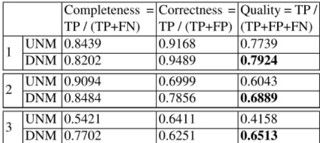
Completeness = TP / (TP+FN) Correctness = TP / (TP+FP) Quality = TP / (TP+FP+FN) 1 UNM 0.8439 0.9168 0.7739 DNM 0.8202 0.9489 0.7924 2 UNM 0.9094 0.6999 0.6043 DNM 0.8484 0.7856 0.6889 3 UNM 0.5421 0.6411 0.4158 DNM 0.7702 0.6251 0.6513
Table 1. Quantitative evaluations of experiments of the three images given in Fig. 4. T, F, P, N, UNM and DNM correspond to true, false, positive, negative, undirected network model and directed network model respectively.
The undirected network model favours network structures in which all branches have the same width. Consequently, network branches which have widths significantly different from the average are not extracted. The result on the third image shows clearly the false negative in the central part of the network branch, where the width is about half the average width. Similarly, the result on the second image shows a false positive at the bottom of the central loop of the network, where the true branch width is small. The result on the first image again shows a small false negative piece in the network junction at the bottom.
The directed network model remedies these problems, as shown by the results in the fourth row. The vector field was initialized to be vertical for the first and third images, and horizontal for the second image. 𝜙 and ∣𝑣∣ are initialized at the saddle point of the ultralocal term 𝑊 , except for the third image where ∣𝑣∣ = 1. The third image shows many gaps in the hydrographic network due mainly to the presence of trees. These gaps cannot be closed using the undirected network model. The directed network model can close these gaps because flow conservation tends to prolong network branches. See Table 1 for quantitative evaluations.
5
Conclusion
In this paper, we have conducted a theoretical study of a phase field HOAC model of di-rected networks in order to ascertain parameter ranges for which stable networks exist. This was done via a stability analysis of a long, straight bar that enabled some model parameters to be fixed in terms of the rest, others to be replaced by physically meaning-ful parameters, and lower and upper bounds to be placed on the remainder. We validated the theoretical analysis via numerical experiments. We then added a likelihood energy and tested the model on the problem of hydrographic network extraction from multi-spectral VHR satellite images, showing that the directed network model outperforms the undirected network model.
0.5023, −0.8, 0.1926, 0.0387, 2.027, 0.2023, 100, 16.66) and (0.4525, −0.2629, 0.6611, −0.8, 0.3585, 0.0289, 5.12, 0.4224, 10, 22.22).
Fig. 4. From top to bottom: multispectral Quickbird images; ML segmentation; MAP segmenta-tion using the undirected model 𝐸P𝑠; MAP segmentation using the directed model 𝐸P. Regions are obtained by thresholding 𝜙 at 0. (Original images c⃝DigitalGlobe, CNES processing, images acquired via ORFEO Accompaniment Program).
A
Appendix
The functions 𝜇, 𝜈 and 𝐺00are
𝜇 = −3𝑣 4 𝑚 20 + 𝑣2𝑚 2 ( 𝜆22 10(𝜙𝑚+ 1)(−3𝜙𝑚+ 2) + 𝜆21 6 (−3𝜙𝑚+ 1) + 1 3 ) +𝜆04 60(𝜙𝑚+ 1) 2(−9𝜙2 𝑚+ 12𝜙𝑚+ 1) + 𝜆03 6 (𝜙𝑚+ 1) 2(−𝜙 𝑚+ 1) + 1 24(𝜆22+ 𝜆21)(𝜙𝑚+ 1) 2 (11) 𝜈 = 𝑣 4 𝑚 4 + 𝑣2𝑚 2 ( 𝜆22 2 (𝜙 2 𝑚− 1) + 𝜆21(𝜙𝑚− 1) − 1 ) +𝜆04 4 (𝜙 2 𝑚− 1) 2 +𝜆03 3 (𝜙𝑚+ 1) 2(𝜙 𝑚− 2) − 1 8(𝜆22+ 𝜆21)(𝜙𝑚+ 1) 2 (12) 𝐺00= 2 ˆ 𝑤2 ∫ +∞ 0 ∫ 𝑤ˆ 0 𝑑𝑧 𝑑𝑥2 ∫ 𝑤−𝑥ˆ 2 −𝑥2 𝑑𝑡 𝛹 (√𝑧2+ 𝑡2) − 𝛹 (√𝑧2+ ( ˆ𝑤 0+ 𝑡)2) (13)
Acknowledgement. The authors thank the French Space Agency (CNES) for the satel-lite images, and CNES and the PACA Region for partial financial support.
References
1. Chen, Y., Tagare, H., Thiruvenkadam, S., Huang, F., Wilson, D., Gopinath, K., Briggs, R., Geiser, E.: Using prior shapes in geometric active contours in a variational framework. IJCV 50 (2002) 315–328
2. Cremers, D., Kohlberger, T., Schn¨orr, C.: Shape statistics in kernel space for variational image segmentation. Pattern Recognition 36 (2003) 1929–1943
3. Paragios, N., Rousson, M.: Shape priors for level set representations. In: ECCV, Copen-hagen, Danemark (2002)
4. Srivastava, A., Joshi, S., Mio, W., Liu, X.: Statistical shape analysis: Clustering, learning, and testing. IEEE Trans. PAMI 27 (2003) 590–602
5. Riklin Raviv, T., Kiryati, N., Sochen, N.: Prior-based segmentation and shape registration in the presence of perspective distortion. IJCV 72 (2007) 309–328
6. Taron, M., Paragios, N., Jolly, M.P.: Registration with uncertainties and statistical modeling of shapes with variable metric kernels. IEEE Trans. PAMI 31 (2009) 99–113
7. Vaillant, M., Miller, M.I., Younes, A.L., D, A.T.: Statistics on diffeomorphisms via tangent space representations. NeuroImage 23 (2004) 161–169
8. Rochery, M., Jermyn, I., Zerubia, J.: Higher order active contours. IJCV 69 (2006) 27–42 9. Rochery, M., Jermyn, I.H., Zerubia, J.: Phase field models and higher-order active contours.
In: ICCV, Beijing, China (2005)
10. El Ghoul, A., Jermyn, I.H., Zerubia, J.: A phase field higher-order active contour model of directed networks. In: NORDIA, in conjunction with ICCV, Kyoto, Japan (2009)
11. El Ghoul, A., Jermyn, I.H., Zerubia, J.: Segmentation of networks from VHR remote sensing images using a directed phase field HOAC model. In: ISPRS / PCV, Paris, France (2010) 12. El Ghoul, A., Jermyn, I.H., Zerubia, J.: Phase diagram of a long bar under a higher-order
active contour energy: application to hydrographic network extraction from VHR satellite images. In: ICPR, Tampa, Florida (2008)