HAL Id: insu-01171195
https://hal-insu.archives-ouvertes.fr/insu-01171195
Submitted on 3 Jul 2015
HAL is a multi-disciplinary open access
archive for the deposit and dissemination of
sci-entific research documents, whether they are
pub-lished or not. The documents may come from
teaching and research institutions in France or
abroad, or from public or private research centers.
L’archive ouverte pluridisciplinaire HAL, est
destinée au dépôt et à la diffusion de documents
scientifiques de niveau recherche, publiés ou non,
émanant des établissements d’enseignement et de
recherche français ou étrangers, des laboratoires
publics ou privés.
whistler waves
O. V. Agapitov, A.V. Artemyev, D Mourenas, Y Kasahara, V Krasnoselskikh
To cite this version:
O. V. Agapitov, A.V. Artemyev, D Mourenas, Y Kasahara, V Krasnoselskikh. Inner belt and slot
re-gion electron lifetimes and energization rates based on AKEBONO statistics of whistler waves. Journal
of Geophysical Research Space Physics, American Geophysical Union/Wiley, 2014, 119, pp.2876-2893.
�10.1002/2014JA019886�. �insu-01171195�
Citation:
Agapitov, O. V., A. V. Artemyev, D. Mourenas, Y. Kasahara, and V. Krasnoselskikh (2014), Inner belt and slot region electron lifetimes and ener-gization rates based on AKEBONO statistics of whistler waves, J. Geophys. Res. Space Physics, 119, 2876–2893, doi:10.1002/2014JA019886.
Received 18 FEB 2014 Accepted 4 APR 2014
Accepted article online 7 APR 2014 Published online 24 APR 2014
and Kp > 3). In particular, the present study focuses on the inner zone L ∈ [1.4, 2] where reliable in situ
measurements were lacking. Such statistics are critically needed for an accurate assessment of the role and relative dominance of each type of wave in the dynamics of the inner radiation belt. While VLF waves seem to propagate mainly in a ducted mode at L ∼ 1.5–3 for Kp < 3, they appear to be substantially unducted during more disturbed periods (Kp > 3). Hiss waves are generally the most intense in the inner belt, and lightning-generated and hiss wave intensities increase with geomagnetic activity. Lightning-generated wave amplitudes generally peak within 10◦of the equator in the region L < 2 where magnetosonic wave amplitudes are weak for Kp< 3. Based on this statistics, simplified models of each wave type are presented. Quasi-linear pitch angle and energy diffusion rates of electrons by the full wave model are then calculated. Corresponding electron lifetimes compare well with decay rates of trapped energetic electrons obtained from Solar Anomalous and Magnetospheric Particle Explorer and other satellites at L ∈ [1.4, 2].
1. Introduction
Satellites are known to be subject to failures caused by MeV electron fluxes trapped in Earth’s radiation belts and often intensified during magnetic storms [e.g., see Horne et al., 2013a]. Many of these satellites are actually orbiting at low altitudes in the region L< 2 where energetic electrons can damage electronic com-ponents via integrated dose or single-event effects [Horne et al., 2013a]. Therefore, accurately calculating and forecasting the dynamical evolution of the energetic electron fluxes trapped in the inner region, L≤ 2 is of a great interest for both satellite design and protection. However, such radiation belt calculations, which are performed by means of massively parallel computations with dedicated codes solving the Fokker-Planck diffusion equation, make use of quasi-linear diffusion coefficients [Kennel and Petschek, 1966; Lyons et al., 1972] to take into account the various effects of wave-particle interactions [e.g., see Subbotin et al., 2011;
Su et al., 2011; Horne et al., 2013a, and references therein]. Thus, these codes require a precise knowledge of
the distribution of the whistler mode waves which are able to scatter particles into the loss cone (leading to their loss in the atmosphere) or to diffuse them in energy.
The present study will mainly focus on the inner region of the plasmasphere comprising the inner electron belt and one part of the slot from L ∼ 1.4 to L ∼ 2 where reliable wave statistics are still lacking [Meredith
et al., 2012; Agapitov et al., 2013; Horne et al., 2013b]. Following early observations of wave-induced
precip-itations [see Vampola and Kuck, 1978; Koons et al., 1981; Voss et al., 1984; Inan et al., 1984, and references therein], Abel and Thorne [1998, 1999] later demonstrated that VLF waves radiated from lightning discharges and terrestrial transmitters should play a major role in determining electron loss timescales in this region. In the absence of reliable in situ statistics, ground-based measurements and rough statistics of these waves combined with approximate transionospheric attenuations and ray tracing have been used to estimate the local wave power in this domain of the radiation belts [Abel and Thorne, 1998; Kulkarni et al., 2008]. However, the accuracy of these estimates has recently been called into question, with several reports of a possible error of up to 1 order of magnitude concerning the actual value of the wave power [e.g., see Graf et al., 2013]. Apart from these estimates, the Space Weather community has until today relied almost exclusively on the
Combined Release and Radiation Effects Satellite (CRRES) data, which have only been published for L ≥ 2 and rely on some additional assumptions to deduce the magnetic component of the wave field from its measured electric component [Meredith et al., 2007].
In the next section, we present new wave amplitude statistics obtained from fitting time-averaged data from the EXOS-D (Akebono) satellite [Kimura et al., 1990], which provides a very good coverage of the critical miss-ing domain L ∼ 1.3–2 (as well as for L ∼ 2–5) for waves ranging from hiss to VLF. It is a worthy complement to other available databases limited to the region L ≥ 2 only. When other wave statistics from the recently launched Van Allen Probes will become available too, some intercomparisons between these two data sets should become worthy of interest. Moreover, we provide here some useful tables of the root-mean-square (RMS) magnetic amplitude Bw(L) of the different waves, obtained after averaging over magnetic local time
(MLT) for L ∈ [1.4, 2.25]. In general, the latitudinal variation of wave intensity will be shown to remain weak for hiss, as well as for lightning-generated waves at latitudes𝜆 > 10◦. Wave amplitudes obtained from Akebono are further compared with wave amplitudes measured onboard satellites CRRES and Dynamics Explorer 1 (DE-1) [Gurnett and Inan, 1988] in the overlapping domain L ∈ [2, 2.5]. In the third section, the effects of the measured whistler mode waves at L ∈ [1.4, 2] on the trapped electron fluxes are addressed by means of numerical calculations of the corresponding quasi-linear pitch angle and energy diffusion coef-ficients. Finally, the resulting electron lifetimes are compared with trapped flux decay rates measured by Solar Anomalous and Magnetospheric Particle Explorer (SAMPEX) [Baker et al., 2007] and other satellites at
L ∈ [1.4, 2], demonstrating a reasonable overall agreement.
2. Spacecraft Statistics
2.1. Satellite Coverage
The EXOS-D (Akebono) spacecraft was launched on 22 February 1989 into an eccentric polar orbit with an initial apogee of 10,500 km, a perigee of 272 km, an inclination of 75.1◦, and an orbital period of 212 min [Takagi et al., 1993], primarily to investigate phenomena associated with the acceleration of auroral particles. Apart from the auroral imager whose CCDs were degraded by the harsh radiation environment in early 1995, all onboard instruments are still healthy and operational. Scientific results obtained from this spacecraft include, among others, the demonstration of particle acceleration by an electric field parallel to geomag-netic field lines [Abe et al., 1991], a quantitative study of ion outflow from the polar ionosphere [Abe et al., 1993], and the discovery and investigation of the characteristics of equatorial magnetosonic waves [Kimura
et al., 1990; Kasahara et al., 1994].
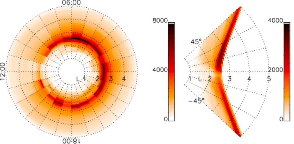
In the present study, we shall only use the measurements of the VLF sensor, which records plasma waves from a few Hz to 17.8 kHz [Kimura et al., 1990; Hashimoto et al., 1997]. The electric components of the plasma wave are taken from two sets of crossed dipole antennas with a total length of 60 m. The mag-netic field components of the wave are measured by three orthogonal loop antennas and three orthogonal search coils for frequencies above and below 800 Hz, respectively. The signals detected by the electric and magnetic sensors are processed on board by a subsystem in the VLF instruments. In this paper, we only considered the data obtained from the following subsystems: (1) the multichannel analyzer (MCA), which measures one component of E and B fields at 16 frequency points between 3.18 Hz and 17.8 kHz, and (2) the wide-band receiver, which is an analog receiver for one component of E or B field below 15 kHz. The cover-age of Akebono measurements is shown in Figure 1 for moderate geomagnetic activity conditions (Kp≤ 3). Such coverage is well adapted for measurements inside the plasmasphere at L ∼ 1.4–3, but only high latitudes are well covered outside of the plasmasphere at L> 3.5. This will probably lead to a relative over-estimation of average chorus amplitudes in the trough, since they are known to peak around𝜆 = 15◦–25◦ [Agapitov et al., 2013; Artemyev et al., 2013a]. The number of available wave measurements at L≤ 2 is about 3⋅ 106for K
p< 3 and 1.5 ⋅ 106for Kp> 3. 2.2. Wave Measurements Onboard Akebono
More specifically, our main goal is to study the distribution over L shells and latitudes of the root-mean-square (RMS) amplitudes of whistler mode waves corresponding to plasmaspheric hiss (0.1–1.5 kHz) [Thorne et al., 1973], lightning-generated (LG) waves (1.5–10 kHz) [Helliwell, 1969; Inan et al., 2007, 2010], and waves produced by terrestrial VLF transmitters (10–23 kHz) [Helliwell, 1969; Smith and
Angerami, 1968]. These three separate frequency ranges are only approximate ones, but they correspond to
Figure 1. The covering of the inner magnetosphere by AKEBONO measurements in 1989–1998 forKp= 0–3. The (left) MLT coverage and (right) latitudinal coverage are shown, respectively. Colors show the number of measurements.
et al., 2013b]. Moreover, our study will mostly focus on the inner region of the plasmasphere comprising the
inner electron belt and one part of the slot from L ∼ 1.4 to L ∼ 2, where detailed statistics of such waves are still lacking. The present section will provide a quick statistics of these waves as measured by Akebono over the range 2.7 to 20.5 kHz at L = 1.4–2.25, usefully supplementing already available databases [Agapitov et
al., 2013; Horne et al., 2013b].
One peculiar feature of the VLF detector onboard Akebono is its covering of the wide range of frequencies from about 3 Hz to ∼21 kHz by 16 separate channels with wide bandwidths ∼0.3 times the channel’s cen-tral frequency and an effective passband (for nominal gain) ∼0.3 times the cencen-tral frequency. However, this makes it sometimes impossible to discriminate between wave modes by their frequencies alone; there may be several wave modes in one channel, especially at high L > 2.5 where chorus, VLF waves from transmit-ters, magnetosonic, and LG waves might coexist. The frequencies𝜔 of all these waves are much smaller than the local electron gyrofrequency Ωce, which is itself smaller than the plasma frequency Ωpenear the equa-tor for L > 1.4. In general, however, all the aforementioned wave types have distinct frequency ranges or different regions (or conditions) of generation and thus can be distinguished in the statistical analysis. One such problem concerns the discrimination between similar-frequency very oblique fast magnetosonic waves [Kasahara et al., 1994; Nˇemec et al., 2005] and mostly parallel hiss waves. But Cluster observations show that (i) fast magnetosonic waves are mainly present at L > 2, with rapidly decreasing occurrences and average intensity as L decreases and (ii) they appear to be confined to latitudes𝜆 < 2.6◦at L < 2.5 [Mourenas et al., 2013]. Moreover, previous CRRES statistics at L ∼ 2 and Cluster statistics at L ∼ 2.25 have demonstrated that magnetosonic wave amplitudes are much smaller than hiss amplitudes during low geo-magnetic activity periods [Meredith et al., 2009; Mourenas et al., 2013]. Thus, we can simply assume in the following that all of the observed waves at low frequencies 200 Hz to 2 kHz over the range L = 1.4–2.2 when
Kp < 3 are really plasmaspheric hiss waves. Still, some waves at high latitudes will actually be lower hybrid
waves. We cannot readily discriminate between lower hybrid and VLF waves. In subsequent numerical calcu-lations of diffusion coefficients, however, it will be easy to stop integrating over latitude before the VLF wave frequency reaches the local lower hybrid frequency. To this aim, as well as to provide plots as a function of normalized frequencies, we make use of the local equatorial electron gyrofrequency Ωce0obtained from the
International Geomagnetic Reference Field and Tsyganenko models (from now on, subscripts “0” indicate equatorial values).
2.3. Measured Wave Amplitude Distributions: Overview
Let us give a brief overview of the general statistics of the waves measured by Akebono. The distribution of latitudinally averaged RMS wave amplitudes Bwis displayed in Figure 2 as a function of L for different
fre-quency channels of the MCA VLF detector of Akebono, separately in the night and day sectors, during low geomegnatic activity (Kp < 3). At L ∼ 1.3 to 2.25, one can notice the similar amplitudes of low-frequency
hiss waves (≤ 1 kHz) on the nightside and on the dayside, contrasting with the much higher amplitude of higher-frequency LG and VLF waves in the night sector than in the day sector. Higher LG wave amplitudes on the nightside are fully consistent with a lower attenuation of electromagnetic waves along their path
Figure 2. Distributions of RMS wave amplitudes averaged over latitude (0◦–30◦) forKp< 3as a function ofLin eight different frequency channels. Day and night sectors correspond to filled circles and empty circles, respectively.
through the ionosphere during the night, as the plasma density is then lower than during the day [Helliwell, 1965; Nˇemec et al., 2010]. Wave amplitudes decrease roughly like 1∕𝜔3∕4as frequency increases at L < 3,
except for the VLF waves. Thus, hiss waves are the most intense, with RMS amplitudes Bw∼10 pT. RMS
ampli-tudes of observed LG and VLF waves are small (∼0.2–1 pT) when Kp < 3, with 10% to 20% occurrence rates
on the nightside at L< 2. At L ∼3–5, measurements are mainly restricted to off-equatorial regions and lower band chorus waves with frequencies ∼1 to 4 kHz generated outside the plasmapause dominate at L> 3.5–4 with higher amplitudes (> 5 pT) at higher L shells, in agreement with Cluster statistics [Agapitov et al., 2013]. The full wave data obtained in these different frequency channels have been further averaged over MLT; then, mean-square-root polynomial fits of the wave amplitude as a function of latitude have been obtained in each frequency range and for L values ranging from 1.3 to 5 (with a step of 0.1), under the form log10(Bw) =
∑i=5
i=0ai𝜆iwith𝜆 in degrees and Bwin pT, for both Kp < 3 and Kp > 3. The
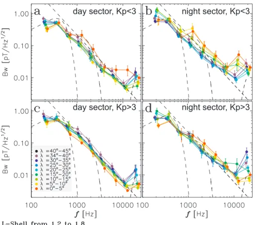
correspond-ing RMS wave spectral density has been plotted in Figure 3 after averagcorrespond-ing over L ∈ [1.2, 1.8] for the day and night sectors separately. Amplitudes are displayed as a function of frequency and latitude upward from the equator in two geomagnetic activity ranges (Kp < 3 and Kp > 3). The empirical fits provided by
Meredith et al. [2007] for L ∼ 2 for hiss and LG waves have been superimposed for comparison purposes.
The latter consist of two Gaussians: ∼ 0.7 exp(−0.5(f − 350)2∕2002) pT∕Hz1∕2from 100 Hz to 1 kHz and
∼ 0.2 exp(−0.5(f − 1000)2∕8002) pT∕Hz1∕2from 1 kHz to 3 kHz, with f the wave frequency in Hz [Meredith et
al., 2007]. We also superimposed two more rough fits for the remaining LG and VLF waves: ∼ 9.5 ⋅ 104⋅ f3∕2
pT∕Hz1∕2from 3 to 13 kHz and a Gaussian ∼ 0.01 exp(−0.5(f − 20, 000)2∕3, 0002) pT∕Hz1∕2from 13 kHz to
23kHz. Such dependences appear legitimate for Kp < 6 at L < 1.8 but only for low geomagnetic activity
Kp < 3 at L < 3 because an additional presence of chorus waves (due to a closer plasmapause) may
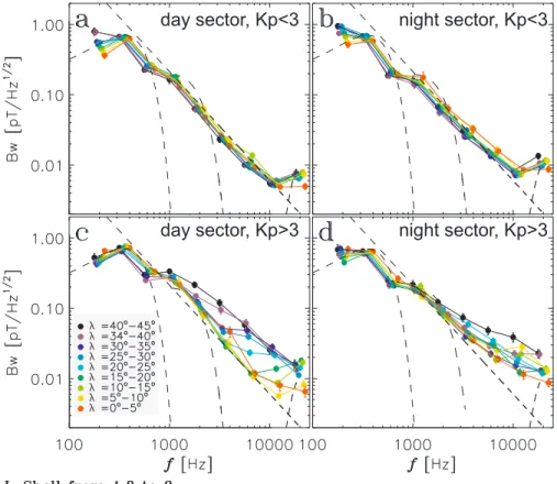
other-wise increase the wave power in the range from 1 kHz to 8–10 kHz, as it is indeed the case in Figure 4 (where spectral density has been averaged over L = 1.8–3). Akebono statistics of hiss and LG wave amplitudes at
L = 1.2–3 are therefore consistent with CRRES fits and results obtained in the narrower range L = 2–2.5
[Meredith et al., 2007] during periods of low geomagnetic activity.
2.4. Measured Wave Amplitude Distributions: Hiss and LG Waves
It is worth emphasizing that there is no indication of any significant dependence of hiss RMS amplitudes on latitude (for f < 1 kHz), consistent with Cluster and CRRES observations at L > 2 [Agapitov et al.,
Figure 3. RMS wave spectral density as a function of frequency forL = 1.2to1.8in the day and night sectors. Ampli-tudes are plotted as a function of latitude averaged over5◦with5◦steps upward from the equator (from red to black). Geomagnetic activity rangesKp< 3andKp> 3correspond to top and bottom, respectively. Dashed curves correspond to empirical fits of Meredith et al. [2007] forL ∼ 2for hiss and LG waves (see text).
2013; Artemyev et al., 2013b; Meredith et al., 2007]. We shall later build on this important fact to provide latitude-averaged hiss amplitudes. As shown in Figures 3 and 4, hiss amplitudes do not increase strongly with geomagnetic acitvity from the range Kp< 3 to the range Kp> 3, at least at low L < 2. Between 1 kHz
and 7.5 kHz, LG waves RMS amplitudes vary with latitude by about a factor of 2 (decreasing with latitude), with almost no variation for𝜆 > 10◦after averaging over MLT. Actually, Cluster observations have shown that waves with frequencies ∼200 Hz to 2 kHz near the equator may also consist of very oblique fast mag-netosonic waves (also called equatorial noise) [Nˇemec et al., 2005; Mourenas et al., 2013]. But magmag-netosonic wave intensity should be small (≤ 1 pT) in general at L < 2 when Kp< 3, with quickly dropping intensities
at frequencies𝜔 > 𝜔LH∕4 [e.g., see Meredith et al., 2009; Mourenas et al., 2013], i.e., for frequencies larger
than about 1 kHz for L ∈ [1.5, 2]. Cluster measurements have also shown that magnetosonic wave power decreases fast at𝜆 > 3◦for L < 2.5 [Mourenas et al., 2013]. In contrast, the increase near the equator of the RMS amplitude of waves in the LG frequency range measured by Akebono occurs from 1 kHz up to 5kHz. Moreover, this increase is present up to𝜆 ∼ 10◦on the nightside (see Figure 2). All these facts taken together suggest that the considered waves are mainly LG whistlers. The higher intensity of these waves at𝜆 < 10◦may be due to their more efficient ducting at lower latitudes in this region. At higher latitudes, whistler mode waves tend to propagate toward higher plasma density regions and then get reflected and further spread out over the whole L = 1.2–3 domain, which could indeed diminish their average intensity. Thus, it appears that one may use a constant RMS amplitude Bw(L) (averaged over both latitude and MLT) for
LG waves when calculating loss rates of energetic electrons at L< 2, but only at latitudes 𝜆 > 10◦. Between the equator and 10◦, the measured variation of wave power should also been taken into account, since it can have an important effect on the minima of diffusion rates at high-equatorial pitch angles𝛼0 > 60◦(which often determine electron lifetimes at low energy; see section 3.1 and the works by Albert and Shprits [2009] and Artemyev et al. [2013b]).
Figure 4. The same as in Figure 3 but forL = 1.8to3.
2.5. Measured Wave Amplitude Distributions: VLF Waves
RMS amplitudes of VLF waves (7.5–21.5 kHz) can be seen to vary with latitude in Figure 3 for L < 1.8. For Kp < 3, the higher-frequency part above 15 kHz remains almost constant (within error bars) as
lati-tude varies, while the portion around 10 kHz (which may partly consist of LG waves) decreases rapidly with latitude between𝜆 = 0 and 𝜆 = 10◦, remaining roughly constant afterward after averaging over MLT. Con-versely, for L > 1.8 and Kp < 3, Bw(𝜆) varies by less than 20% around the mean value (see Figure 4). Thus,
using the latitudinally averaged RMS amplitude of VLF waves seems to be a reasonable approximation for calculating electron scattering during geomagnetically quiet or moderately active periods such that Kp< 3, but again, only for𝜆 > 10◦at L< 2. At lower latitudes, the observed variation of wave power must also be taken into account.
For VLF (∼15 kHz) waves, the Gendrin and resonance cone angles𝜃g = arccos(2𝜔∕Ωce) and𝜃r = arccos(𝜔∕Ωce) are such that𝜃g ∼ 70◦–80◦near the equator for L = 1.5–2 and 𝜃g < 70◦at higher L > 2. Therefore, the moderate latitudinal dependence of VLF wave amplitude for L = 1.4–3 during low geomag-netic activity suggests that wave-normal angles do not increase strongly during wave propagation from low-altitude entry (i.e., high latitude) up to the equatorial plane. It corresponds to a mainly ducted propa-gation of VLF waves at L = 1.5–3 for Kp < 3, in agreement with many past studies [e.g., see Cerisier, 1974;
Burgess and Inan, 1993; Clilverd and Horne, 1996; Clilverd et al., 2008; Rodger et al., 2009, 2010, and
refer-ences therein]. Similarly, high-frequency LG waves (>5 kHz) are probably mostly ducted at L > 2.5, which agrees well with the reported absence of wave propagation above the electron half-gyrofrequency limit at such high frequencies [Nˇemec et al., 2010; Smith et al., 1960]. However, no definite inference can be drawn from the weak-latitude dependence of amplitudes for lower frequency waves, because their Gendrin and resonance cone angles are much closer to 90◦.
Conversely, during highly disturbed periods (Kp > 3), the RMS amplitude of VLF waves now increases with latitude by factors ∼2 (for L ∈ [1.8, 3]) to ∼3 (for L ∈ [1.2, 1.8]) between the equator and 𝜆 ∼ 30◦. Latitude-increasing VLF wave amplitudes have also been reported based on DE-1 measurements of 11.8 kHz waves at L ∈ [1.5, 2] [Green et al., 2006]. Such a behavior is consistent with ray-tracing simulations
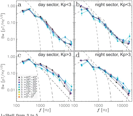
Figure 5. The same as in Figure 3 but forL = 3to5.
of unducted waves showing an increase of the wave-normal angle along propagation, from 30◦at (high-latitude) entry points into the lower magnetosphere up to 50–60◦at the equator [Abel and Thorne, 1998; Kulkarni et al., 2008]. Such an increase of the obliquity of whistler mode waves should indeed be accompanied by a corresponding decrease of their magnetic field component Bw[e.g., see Stix, 1962;
Verkhoglyadova et al., 2010]. Indirect but convincing experimental evidence of a similarly unducted
prop-agation of high-frequency whistlers during geomagnetically disturbed periods has been reported by Peter
and Inan [2004]. In such a case, using a constant latitudinally averaged VLF wave amplitude could lead to
sig-nificant errors in electron scattering rates. A general increase of unducted propagation of VLF waves during disturbed periods does not contradict the results of Thomson et al. [1997], which found a somewhat higher efficiency of ducted transmission of VLF signals for higher Kpat L ∈ [1.8, 2.6]: it simply means that more wave power should be partly (or temporarily) trapped inside ducts during low Kpperiods than it may seem when only studying the signals finally reaching the vicinity of the conjugate region. Moreover, the increase in transmission efficiency observed by Thomson et al. [1997] is much less apparent over the range Kp∈ [2, 5] which represents the major part of any real-time statistics [see Thomson et al., 1997, Figure 6].
Surprisingly, the fits to CRRES average wave spectra obtained at L ∼2 [Meredith et al., 2007] turn out to remain quite close to Akebono spectra measured in the domain L = 3–5 at medium to high latitudes
𝜆 > 10◦–15◦(see Figure 5). But this is true for low geomagnetic activity K
p < 3 only, when the average
plasmapause position is located at L> 4.2 [O’Brien and Moldwin, 2003]. For Kp> 3, the plasmapause comes
closer to the Earth. Then, intense chorus waves generated by strong injections of 30–50 keV electrons from the plasmasheet are seen to dominate the wave spectrum above 1 kHz.
2.6. Simplified Modeling of Observed Waves
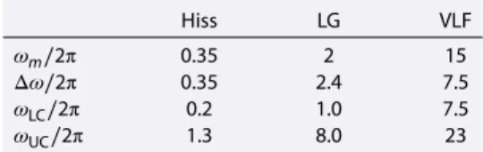
In the next section, we shall use the average wave amplitude statistics from Akebono presented above to calculate electron pitch angle and energy quasi-linear diffusion coefficients, as well as lifetimes. To this aim, the wave spectra have been further approximated by three Gaussians such that B2
w(L, 𝜔) = B2w(L) exp(−(𝜔 −
𝜔m)2∕Δ𝜔2) corresponding to hiss, LG, and VLF waves, with mean frequencies𝜔m, widths Δ𝜔, lower cutoffs
Table 1. Characteristic Frequency Parameters
(in kHz) of the Three Gaussian Fits to Spectra of Measured Hiss (∼0.2–1.3 kHz), Lightning-Generated Whistlers (∼1.3–7.5 kHz) and VLF Waves
(∼7.5–21 kHz) as a Function ofLforKp< 3 Hiss LG VLF 𝜔m∕2π 0.35 2 15 Δ𝜔∕2π 0.35 2.4 7.5 𝜔LC∕2π 0.2 1.0 7.5 𝜔UC∕2π 1.3 8.0 23
Latitudinally averaged RMS wave amplitudes Bw(L)
obtained from one-component measurements onboard Akebono from L = 1.4 to L = 2.25 in the inner belt and slot regions are provided in Table 2 for Kp< 3 and Kp> 3. Note that an additional running average over the closest neighboring L shells has been performed to obtain these values. Hiss wave amplitudes can be assumed as nearly constant as a function of latitude for L< 2. For LG waves at L< 2, however, a constant average amplitude can only be used for𝜆 > 10◦. Closer to the equator (for𝜆 < 10◦), a rough multiplying factor MLG≈ max((10 −𝜆)∕1.3)1∕3, 1)
(with𝜆 in degree) is therefore applied to the average amplitude for L ∼1.4–2 and Kp< 3, to account for the
observed latitudinal variation (at higher L> 2 or for Kp> 3, one may take MLG ∼ 1). For VLF waves at L< 2 and for Kp< 3, the amplitude multiplicative factor becomes MVLF,1≈ max((10 −𝜆)∕2.5)1∕2, 1) for 𝜆 < 10◦.
As concerns VLF waves when Kp > 3, their amplitude variation with latitude can be roughly approximated by a multiplicative factor MVLF,2 ∼ (𝜆∕𝜆max,Ne+ 0.75)𝛽with𝛽 ∼ 1 for L ∼ 1.4–1.9 and 𝛽 ∼ 0.7 for L ∈ [2, 3].
The latitude at which one reaches an altitude of 2000 km on a given field line L is𝜆max,Ne(L): it corresponds
roughly to the maximum latitude of our wave statistics at L< 3. Note that the trapping (or not) of whistler waves into field-aligned ducts of enhanced density is also believed to occur at altitudes ∼2000 km [Helliwell, 1965; Strangeways and Rycroft, 1980; Gorney and Thorne, 1980]. The RMS amplitudes corresponding to the 5% most intense waves recorded onboard Akebono have also been examined. It appears that mea-sured hiss, lightning, and VLF wave amplitudes can increase by factors ∼1.5–2 from their values during low geomagnetic activity periods, which agrees well with results from CRRES at L = 2–3 [Meredith et al., 2007]. The measured MLT-averaged hiss and LG waves RMS amplitudes are in rough agreement with correspond-ing values obtained from DE-1 and CRRES data at L = 2 and L ∼ 2.25, although hiss amplitudes measured by Akebono appear sensibly smaller than CRRES values. Similarly, VLF wave amplitudes from DE-1 compare well with Akebono results at L = 2 and L ∼ 2.25. Hiss waves have the largest amplitudes (around 10–15 pT), while LG and VLF waves have similar RMS amplitudes (Bw∼ 1.5–3 pT). A relative maximum of both LG and
VLF wave amplitude can be seen near L = 1.6, while hiss amplitudes smoothly decrease toward low L shells. The maximum of LG wave intensity at L ∼ 1.6 correlates well with the peak at 𝜆 ≈ 38◦of wave power in the range 3–6 kHz observed on DEMETER [Nˇemec et al., 2010]. In general, the averaged (over MLT and latitude) amplitudes of hiss and LG waves increase only slightly (10% to 30%) from Kp < 3 to Kp > 3 in the domain
L ∈ [1.4, 2], i.e., less than for L > 2 where hiss amplitudes rise 50% to 100% (see Figure 2). The increase of
Table 2. MLT-Averaged and Latitude-Averaged (From∼0◦up to
∼30◦–35◦) RMS Wave Amplitudes (in pT) of the Three Gaussian Fits for Hiss (∼0.2–1.3 kHz), Lightning-Generated Whistlers (∼1.3–7.5 kHz), and VLF Waves (7.5–21 kHz) One-Component Measurements Onboard Akebono, as a Function ofLforKp < 3
andKp> 3, Respectivelya Kp< 3 < 3 < 3 Kp> 3 > 3 > 3 L Hiss LG VLF Hiss LG VLF 1.4 9 1.7 2 8 2.4 2.5 1.5 9 1.9 2.5 11.5 2.2 3 1.6 10 2.2 2.5 11 2.5 3 1.7 12 2.2 2 12 2.5 2 1.8 12 2.5 2 13 2.5 2 2.0 16 2.5 1.5 17 3 2 2.25 15 2.7 1.1 17 3.5 1 2 (CRRES) ∼ 23 ∼ 3 – ∼ 30 ∼ 4 – 2.3 (CRRES) ∼ 29 ∼ 3.6 – ∼ 40 ∼ 4.5 – 2.3 (DE-1) ∼ 12 ∼ 2.5 ∼ 1 ∼ 15 ∼ 3 ∼ 1
aCorresponding values for quiet and active conditions
from CRRES and DE-1, when available, are also indicated [see Artemyev et al., 2013b; Meredith et al., 2007].
plasmaspheric hiss wave power dur-ing magnetically disturbed periods probably originates in the increase of the intensity of hiss-seeding chorus waves generated outside of a closer plasmapause [Bortnik et al., 2008]. The smaller increase at lower L < 2 may be related to a preferential focusing of incoming hiss-seeding chorus waves in more numerous high-density ducts at
L> 2 near the edge of the compressed
plasmasphere [e.g., see Hayakawa and
Tanaka, 1978; Chen et al., 2012], but it
could also be caused by a larger absorp-tion at low altitudes due to an increased electron density. The slight increase of LG wave power could be caused by the partial confinement of these waves into a smaller-volume plasmasphere during disturbed periods or to a small additional presence of 3–6 kHz chorus waves
2 (CRRES) ∼ 23 ∼ 3 – ∼ 30 ∼ 4 – 2.3 (CRRES) ∼ 29 ∼ 3.6 – ∼ 40 ∼ 4.5 –
aFull wave amplitude estimates have been obtained by
mul-tiplying the one-component-onlyBw value measured onboard Akebono by a factor√3to account for the roughly similar aver-age magnitudes of the two remaining orthogonal components, in the general case of oblique wave propagation with respect to the perpendicular to the measured component’s direction. Corresponding values for quiet and active conditions obtained from CRRES one-component electric field measurements are also indicated [see Artemyev et al., 2013b; Meredith et al., 2007].
The average (RMS) wave amplitudes of hiss, LG, and VLF waves measured in situ by Akebono are sensibly different from the estimates used in past studies of trapped electron lifetimes in the slot and inner belt at L ∼ 1.4 to 2 [Abel and
Thorne, 1998, 1999; Albert, 1999]. In this
region, the latter works assumed aver-age hiss amplitudes of ∼3.2 pT, around 3to 5 times smaller than measured val-ues. Average amplitudes of LG waves were also slightly underestimated at ∼2 pT. On the other hand, MLT-averaged VLF wave amplitudes were seemingly sensibly overestimated at Bw ∼ 3.2–4 pT for L = 1.4–2 [Abel and Thorne, 1998; Albert, 1999].
However, recent state-of-the-art simulations of the propagation and attenuation of VLF waves through the ionosphere and into the magnetosphere have shown that the older calculations [Abel and Thorne, 1998;
Albert, 1999] should at most overestimate VLF wave power by less than a few dB [Graf et al., 2013]. This
fact, together with the sensibly larger amplitudes of hiss waves obtained by CRRES from one-component electric field measurements, suggests that the wave amplitudes obtained onboard Akebono from MCA one-component magnetic field measurements may actually be lower than the full (three-component) wave amplitudes. The full magnetic component of parallel and oblique whistler mode waves is located in a plane perpendicular to their wave vector [Verkhoglyadova et al., 2010]. Thus, the full magnetic component of nearly parallel (or ducted) waves lies in a plane nearly perpendicular to the geomagnetic field line. In this case, one-component Bwmeasurements by Akebono are likely to underestimate the full wave amplitude
by a factor ∼√2on average, provided that the measured component is perpendicular to the wave vec-tor. But in the general case of oblique (unducted) whistler mode waves or when the component measured by MCA is not perpendicular to the wave vector, all three orthogonal components of the wave amplitude should have similar average magnitudes. In this more general case, the average full wave amplitude Bwis
expected to be roughly√3times larger than the single measured component provided by Akebono. The corresponding estimates of the full wave amplitudes are given in Table 3 for Kp< 3 and Kp> 3. The obtained
values are both closer to the previous estimates of VLF amplitudes [Abel and Thorne, 1998; Albert, 1999] and to CRRES-derived hiss amplitudes (from electric field measurements). Overall, the higher full wave ampli-tudes together with a more ducted propagation of VLF waves should lead to reduced energetic electron lifetimes as compared to the works by Abel and Thorne [1998, 1999] and Albert [1999]. Detailed calculations and comparisons with observed decay rates are provided in the next section.
Finally, a full model of wave-particle interaction in the inner belt must include upper latitude cutoffs for each wave, as well as a proper model of cold electron density inside the plasmasphere. As regard the cold electron density, we shall simply use the profile obtained by Ozhogin et al. [2012] based on recent Radio Plasma Imager (RPI) measurements inside the plasmasphere. We have further checked that this model gives density values within 10% of the model optimized by Selesnick et al. [2013] for L = 1.5–2. Thus, the plasma density is taken as Ne ∼ 3⋅ 104⋅ 10−L∕2cos−3∕4(1.9𝜆) cm−3as a function of
Table 4. Upper Bounds𝜆max,Ne,𝜆max,LG, and
𝜆max,VLFon the Latitude (in Degrees)
Correspond-ing Respectively to Altitudes Above2000km for the Density ModelNeto be Valid [Ozhogin et al., 2012], and for5kHz LG Waves and20kHz VLF Whistler Mode Waves to Remain Such That
𝜔 > 2√ΩceΩci(Assuming ThatHis the Dominant
Species), as a Function ofLforKp< 3
L 𝜆max,Ne 𝜆max,LG 𝜆max,VLF
1.4 15.5◦ – 16◦ 1.5 21.4◦ – 21◦ 1.6 25.7◦ – 24◦ 1.7 29◦ – 27◦ 1.8 31.8◦ – 28.5◦ 2.0 36.3◦ 4.5◦ 33◦
latter nominal value. The corresponding equatorial electron plasma frequency to gyrofrequency ratio varies between Ωpe0∕Ωce0 ∼ 2.25 and ∼ 4.6 as L
increases from 1.4 to 2. However, this density model is only valid for altitudes above 2000 km. The cor-responding upper bounds on latitude𝜆max,Ne(L) ∼ arccos(√1.3∕L) are provided in Table 4. It is worth emphasizing that this lower limit of altitude of 2000km also corresponds roughly to expected min-imum altitudes (or maxmin-imum latitudes) for wave trapping into ducts [Strangeways and Rycroft, 1980]. It is assumed here that the geomagnetic activity is not too high (i.e., Kp≤ 5) in order for the plasmapause to
stay far enough at L > 3. Based on CRRES measure-ments inside the plasmasphere at L ∈ [3, 5], Sheeley
et al. [2001] have also shown that there was little effect of geomagnetic activity on density. One expects that
it should be even more true at lower L shells.
In general, the latitude integration of quasi-linear diffusion coefficients will be limited in the following at
𝜆 < 𝜆max,Ne(L) for hiss, lightning-generated, and VLF whistler mode waves. But another limit must also be
considered when dealing with very oblique whistler waves (𝜃 > 60◦). Actually, a resonance cone exists only for whistler mode waves such that their frequency is higher than the local lower hybrid frequency
𝜔 > ΩLH∼
√
ΩceΩci, so that the refractive index surface N(𝜃) is open and N can reach large values [Stix, 1962;
Kulkarni et al., 2008; Mourenas et al., 2012b]. The corresponding limits on latitude𝜆max,LG(L) and𝜆max,VLF(L)
are provided in Table 4. One can see that LG wave frequencies are generally too small for having a resonance cone for L < 2. Similarly, hiss frequencies are always smaller than the lower hybrid frequency for L < 2.3. In ensuing scattering rate calculations, the maximum allowed latitude for very oblique VLF waves will be taken as the smaller between the two limits𝜆max,VLF(L) and𝜆max,Ne(L), since no effect of very oblique waves
is expected above such a latitude.
3. Quasi-Linear Scattering Rates and Electron Lifetimes in the Inner Belt (L
< 2)
3.1. Analytical Estimates of Dominant Wave Contributions to Electron Lifetimes
Based on the classic formulation of electron quasi-linear diffusion coefficients [Lyons et al., 1971, 1972;
Lyons, 1974; Glauert and Horne, 2005], approximate useful and insightful analytical expressions of the
bounce-averaged pitch angle and energy scattering rates have been derived under the assumption of quasi-parallel (𝜃 < 45◦) or very oblique (𝜃 > 60◦, 𝜃g) waves in a series of papers [see Mourenas and Ripoll,
2012; Mourenas et al., 2012a, 2012b; Artemyev et al., 2013b; Mourenas et al., 2013]. Moreover, it has been shown that trapped electron lifetimes can also be expressed analytically even in the simultaneous presence of different types of waves [Artemyev et al., 2013b; Mourenas et al., 2013]. Based on Akebono statistics pre-sented above, we consider in the inner belt a spectrum consisting of three Gaussians with the parameters presented in Table 1 for hiss, LG, and VLF whistler waves. Peak frequencies and upper cutoffs of each Gaussian are denoted as𝜔m,iand𝜔UC,i, respectively, where subscript i corresponds to a given wave type. For quasi-parallel waves, the electron lifetime𝜏Lcan be written as the integral over𝛼0of separate contributions
of the different minima in⟨D𝛼0𝛼0⟩
Btan𝛼0[see Albert and Shprits, 2009; Mourenas and Ripoll, 2012; Artemyev
et al., 2013b]. It takes a form
𝜏L≈𝜏Landau+ ln(0.75∕sin 𝛼LC ) 4⟨Dsmall𝛼0, i=j ⟩s B +∑ i=k,lΔ𝜏i (1)
The first term in equation (1) corresponds to electron diffusion via Landau (or Cherenkov) resonance. For this kind of scattering, the dominant wave type is the one with the largest value of B2
w,i(gs(𝜃M0,i) +
min(C3
i∕11, Ci−1)), where tan𝜃M0,i ≈ 1.84∕p𝜀m0,i,𝜀m0,i = (Ωpe∕Ωce0)
√
𝜔mi∕Ωce0, p = (𝛾2 − 1)1∕2is
the dimensionless momentum (with𝛾 the relativistic factor), and Ci = p𝜔
1∕2
m,iΩpe0∕Ω 3∕2
ce0tan Δ𝜃i[see
Artemyev et al., 2013b]. We assume a Gaussian wave-normal angle distribution gs ∼ exp(− tan2𝜃∕ tan2Δ𝜃i)
for quasi-parallel waves with Δ𝜃i ≈ 30◦. The position of the Landau peak near𝛼0 = 90◦is given by
cos𝛼M0,i ≈ |1 − 𝜔m,i∕Ωce0|1∕2𝛾𝜔
waves of higher frequency (but smaller than VLF) should become dominant. Finally, at low L≤ 1.5 and E ≤ 1 MeV, only VLF waves are cyclotron resonant. This second (cyclotron) term in equation (1) varies with L and
Emuch more slowly than the first (Landau) term in general and determines electron lifetimes only at high energies and high L≥ 2 [Mourenas and Ripoll, 2012; Mourenas et al., 2012b].
The third (last) term in equation (1) corresponds to the filling of the trough in pitch angle scattering rate between the Landau and first cyclotron peaks by means of cyclotron resonance scattering by waves other than j such that𝛼UC,i > 45◦(see details in Artemyev et al. [2013b]). Typically, this third term becomes larger
than the second term when tan Δ𝜃k(sin𝛼UC,k− sin𝛼UC,j)B2w,i=j∕(15B2w,k) > p5∕9Ω5∕9 pe0𝜔 7∕9 m,i=j∕(𝜔 1∕2 m,kΩ 5∕6 ce0), where
kcorresponds to the wave type with immediately higher frequency than the j wave. Based on Akebono statistics in Tables 1–3, such a configuration can exist at L≤ 2 for 0.5–2 MeV electrons, especially in the case of a mainly unducted wave-type k such that Δ𝜃k > 45◦. Then, this third term from LG or VLF waves may actually determine electron lifetimes when it is larger than𝜏Landau, for intermediate values of L and E. When quasi-parallel and very oblique waves (𝜃 > 60◦) coexist, as for Kp > 3 at L < 2 where both ducted
and unducted VLF waves have been observed onboard Akebono, the presence of higher-order cyclotron resonances with very oblique waves can strongly increase pitch angle scattering at small𝛼0as compared to
fundamental cyclotron resonance alone for parallel waves [Mourenas et al., 2012b; Artemyev et al., 2013b]. However, their effect on energy scattering rates is much weaker [Lyons, 1974; Mourenas et al., 2012a]. At small L shells, additional losses related to Coulomb collisions must also be taken into account. A corresponding approximate loss timescale𝜏colis [Walt, 1964]
𝜏col[days] ∼
104(L − 1.15)2.36(𝛾2− 1)3∕2
1.9𝛾 . (2)
The above formula for𝜏colhas been checked to yield values at L ∈ [1.4, 1.6] in good agreement with more
recent studies [Selesnick, 2012]. The full electron lifetime can be written as𝜏 ∼ 1∕(1∕𝜏L + 1∕𝜏col) from
equations (1) and (2). In general, collisional losses become important only at low L shells, for L < 1.5. For instance, one has𝜏col∼ 500 and 4500 days at L = 1.4 for E = 0.5 and 2 MeV, respectively, and 𝜏coldecreases
(respectively increases) very fast at lower (respectively higher) Ls.
3.2. Numerical Evaluation of Scattering Rates
Wave-normal angle distributions g(𝜃) consisting of two Gaussians are used to calculate diffusion rates, together with the Appleton-Hartree cold plasma whistler mode dispersion relation [Artemyev et al., 2013a, 2013b]. The numerical scheme is detailed in the works by Glauert and Horne [2005] and Artemyev et al. [2013b]. Realistic plasma density variations with L and𝜆, provided by Ozhogin et al. [2012], are taken into account. Deep inside the plasmasphere, the cold plasma temperature can be assumed as lower than 1 eV: in this case, thermal effects which essentially affect very oblique whistler mode waves near the resonance cone [e.g., see Hashimoto et al., 1977] should remain negligible and are not included in our calculations. It is worth noting that the Appleton-Hartree whistler mode dispersion relation that is used here does not contain any ion term. Therefore, it could become erroneous when the considered wave frequency decreases to values close to the lower hybrid frequency, near which wave reflection eventually occurs at high latitudes [Shklyar
et al., 2004]. Nevertheless, a careful examination of the full dispersion relation [e.g., see Shklyar et al., 2004; Mourenas et al., 2013; Irie and Ohsawa, 2003] shows that the Appleton-Hartree dispersion relation remains
Figure 6. Bounce-averaged pitch angle diffusion coefficients as a function of𝛼0forKp< 3and electron energyE = 0.5,1,2, and5MeV forL = 1.4to2. Black, blue, and red curves correspond respectively to hiss, LG, and VLF wave separate contributions (quasi-parallel propagation) with average one-component wave amplitudes given in Table 2. Dotted red curves show results for VLF as a sum of ducted and unducted waves withBw,2∕Bw,1= 0.1. Green curves correspond to VLF waves with a larger portion of very oblique (unducted) waves withBw,2∕Bw,1= 0.5.
a very good approximation for not-too-oblique whistler mode waves such that cos𝜃 ≫ 𝜔m∕Ωceas long as
the wave frequency𝜔mremains much larger than the ion gyrofrequency Ωci, i.e., for frequencies higher than
200Hz to 300 Hz for 1.4 < L < 2.
In this paper, the wave-normal angle distribution for each wave type is approximated by two Gaussians with mean values and variances: g(𝜃) = g1(𝜃) + g2(𝜃)(Bw,2∕Bw,1)2, where gi = exp(−(𝜃 − 𝜃mi)2∕Δ𝜃i2) and
i = 1, 2, 3. For hiss and LG waves, we use only one Gaussian with 𝜃mi = 15◦and Δ𝜃i ≈ 10◦appropriate for
not-too-oblique waves, while for VLF waves we use two Gaussians, one for quasi-parallel waves being sim-ilar to the one just described above and a second one with𝜃mi ∼ 75◦and Δ𝜃i = 10◦(as done previously
in the work by Artemyev et al. [2013a]). Note that the hiss and LG wave-normal distributions roughly corre-sponds to𝜃 distributions for hiss and LG waves at L ∼ 2.2 and 𝜆 < 20◦obtained from Cluster measurements [Artemyev et al., 2013b]. For VLF waves, to properly take into account the presence of ducted (quasi-parallel) waves likely accompanied by some population of unducted (oblique) waves [Clilverd et al., 2008; Kulkarni et
al., 2008; Rodger et al., 2010], the amplitude ratio Bw,2∕Bw,1is taken as 0 (i.e., quasi-parallel waves only), 0.1 [ see Artemyev et al., 2013a, 2013b], and finally, 0.5 (representing significantly unducted VLF waves). In the latter case, we shall also use slightly larger VLF Gaussians with Δ𝜃 ≈ 14◦to better model the wave-normal angle distribution of unducted VLF waves.
The g(𝜃) distribution used here represents a satellite-measured wave-normal angle distribution. It already contains one sin𝜃 term which appears inside the 𝜃 integrals of diffusion coefficients [Lyons et al., 1971]. When using our g(𝜃) distributions, one sin 𝜃 term must therefore be removed in each 𝜃 integral of the usual expressions of the diffusion coefficients to calculate scattering rates.
Figure 7. Total bounce-averaged pitch angle and energy diffusion coefficients as a function of𝛼0forKp < 3and electron energyE = 0.5,1,2, and5MeV for
L = 1.4to2. The measured (one-component) average wave amplitudes given in Table 2 are used. Black and grey dotted lines indicate the bounce loss cone and approximate drift loss cone positions, respectively.
Figure 4 shows the bounce-averaged quasi-linear pitch angle diffusion coefficients calculated for hiss, LG, and VLF waves separately, for different L shells and electron energies, one the basis of the modeled ampli-tudes (one-component only) provided in Table 2 for Kp < 3. As expected from analytical estimates in
section 3.1, one finds a dominance of hiss cyclotron scattering at high L and high-electron energy, followed successively by LG and VLF at lower and lower L and E. As predicted too, the minimum of diffusion at large pitch angles is generally dominated by LG or VLF cyclotron scattering at L ∼1.8–2. The maximum pitch angle
𝛼0 ∼𝛼UCfor cyclotron resonance with a given wave decreases as frequency, L, or E decrease, in agreement
with analytical estimates. At small L < 1.6 and E < 1 MeV, one can notice an important effect of the pos-sible presence of very oblique (unducted) VLF waves. Such waves may increase significantly the scattering rates, especially near their minima, which could entail reduced lifetimes at L < 1.6 for E < 1 MeV. Nev-ertheless, it occurs only for a large amount of oblique VLF waves (Bw,2∕Bw,1 ∼ 0.5) and only at L < 1.6 where the additional effect of Coulomb collisions already limits efficiently the maximum lifetimes at low energy to similar or even lower levels. Thus, we shall only consider in the following nearly parallel waves. The total bounce-averaged pitch angle and energy diffusion coefficients obtained by summing over all the wave contributions are displayed in Figure 7 as a function of L and E. However, the estimated full wave amplitudes (three-components) given in Table 3 should probably be used to get more realistic estimates of actual scattering rates. The latter can readily be obtained by simply multiplying the levels in Figures 4–7 by a factor 3.
The equilibrium structure of the inner electron radiation belt has been explained by slow inward radial diffu-sion from an outward source together with losses by Coulomb collidiffu-sion and wave-particle interaction [Lyons
and Thorne, 1973]. However, Kim and Shprits [2012], by examining radial profiles of the phase space density
(PSD) of 1–2 MeV electrons measured by three satellites, have shown that there is a clear local peak and a negative radial gradient in the outer portion of the inner zone. It means that either some local acceleration process is at work at L ∼ 1.5 or that the inner electron belt is formed by occasional injections during highly disturbed periods [Kim and Shprits, 2012]. Actually, Horne et al. [2005] have demonstrated that whistler mode chorus waves such that𝜔m∕Ωce0 ∼ 0.1–0.3 can efficiently accelerate high pitch angle electrons to
the MeV energy range outside of the plasmasphere. But what about the inner belt? Making use of Akebono wave statistics in this region, the calculated energy scattering rates at large pitch angles𝛼0∼ 50◦–80◦show
a small relative maximum at L ∼ 1.5 for E = 1 MeV in Figure 7. But no similar maximum can be seen at 2MeV. However, the effect of trapped electron losses on energization must also be taken into account before drawing any definitive conclusion. This point will be addressed in the next section.
3.3. Resulting Electron Lifetimes
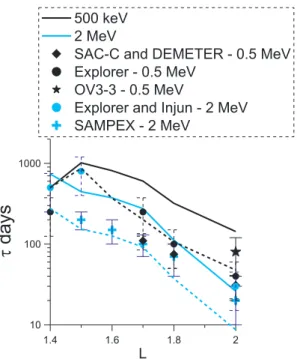
Electron lifetimes𝜏 calculated numerically with the modeled distributions of hiss, LG, and VLF wave ampli-tudes obtained from Akebono can be compared with measurements of trapped electron decay rates performed onboard SAMPEX [Baker et al., 2007], SAC-C and DEMETER [Benck et al., 2010], as well as Explorer
Figure 8. Electron lifetimes atE = 0.5MeV and2MeV forL = 1.4
to2during moderate geomagnetic activity periods (Kp < 3). Solid and dashed curves are calculated respectively with the mea-sured one-component average wave amplitudes given in Table 2 and with the estimates of the average full wave amplitudes pro-vided in Table 3. VLF waves are assumed to be mainly ducted near the equator. The corresponding decay rates measured by SAM-PEX, SAC-C and DEMETER, and Explorer, Injun and OV3-3 satellites are indicated by different symbols, together with corresponding errors bars.
and Injun satellites [Van Allen, 1964; Abel
and Thorne, 1998] and OV3-3 [Benck et al.,
2010]. Coulomb collisions are taken into account via equation (2), while the electron loss rate𝜏Linduced by whistler wave
scatter-ing is calculated numerically by integration of 1∕(4⟨D𝛼0𝛼0⟩Btan𝛼0) from the drift loss cone
up to 89◦.
Figure 8 shows a comparison between elec-tron lifetime calculations based on Akebono measurements of whistler waves at L ∈ [1.4, 2] and the lifetimes measured by vari-ous satellites during moderately disturbed periods (Kp < 3) for E = 0.5 MeV and 2 MeV.
There is a rough quantitative agreement between the calculated and measured val-ues when using the estimates of the (average) full wave amplitudes (i.e., three-component amplitudes) provided in Table 3. Taking into account the usual variation of lifetimes inferred from measurements by a factor ∼1.5–2 around their plotted mean values [Baker et al., 2007; Benck et al., 2010], it can be considered on the whole as a satisfac-tory agreement. As expected from analytical estimates in section 3.1, hiss wave cyclotron resonance scattering determines electron life-times at high L ∼ 2 and high E ∼ 5 MeV, VLF wave Landau resonance scattering dominates at low L ∼ 1.4–1.6 and low E ∼ 0.5 MeV together with collisional losses, while cyclotron diffusion by LG waves becomes important in the intermediate parameter range.
It is also worth noting the good qualitative agreement between the measured and calculated increases of lifetimes toward lower Ls, as well as the good agreement between the measured and calculated life-time decreases as E increases from 0.5 to 2 MeV at L > 1.6. It is plain to see that using only the measured one-component wave amplitudes given in Table 2 leads to a general overestimation of measured lifetimes by a factor 2 to 4. This fact is consistent with our assumption that full wave intensities should be on aver-age ≈ 3 times larger than the measured single components, especially as concerns VLF waves which are principally responsible of the lifetime levels at low energy (see Figures 4–7).
Note that the powerful North West Cape (NWC) transmitter at 22.3 kHz (during the considered Akebono measurements) was not yet in operation in the 1960s when Explorer and Injun satellite measurements were performed. It could be the reason that electron lifetimes at low energy and low L obtained by these satel-lites are higher than the values obtained more recently by SAMPEX, SAC-C, and DEMETER. Nevertheless, it should be noted that lifetimes at E = 500 keV from SAC-C and DEMETER agree well with lifetimes derived from Explorer measurements for L ∼ 1.8–2, although they are twice smaller at L ∼ 1.7. The spread of the measured lifetimes stems more probably from the natural variation of the wave∕plasma conditions in rela-tion with the actual geomagnetic activity at the time of the measurements. While the operating frequency of the NWC transmitter falls inside the bandwidth of the last frequency channel of Akebono (which goes up to 23 kHz), it lies outside its effective nominal-gain passband. Accordingly, the corresponding wave intensity should be underestimated here by a factor< 1∕3.
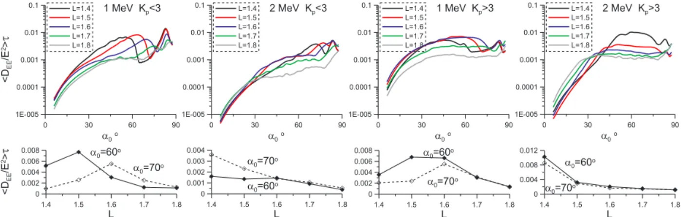
Figure 9 displays the important factor (𝜏 ⟨DEE⟩B∕E2) defining the regime of electron energization at L =
1.4–1.8 [Artemyev et al., 2013a]. It appears that (𝜏 ⟨DEE⟩B∕E2)≪ 1 for E = 1–2 MeV. It means that electron
acceleration by LG and VLF waves occurs in a loss-dominated regime. In such a case, energization increases with the increase of (𝜏 ⟨DEE⟩B∕E2). Therefore, Figure 9 shows that electron energization by diffusive resonant
Figure 9. The factor(𝜏 ⟨DEE⟩B∕E2)plotted for two geomagnetic activity ranges and two energiesE = 1and2MeV atL = 1.4to1.7. VLF waves are assumed to be
mainly ducted. (top) Display of𝜏L⟨DEE⟩B∕E2as a function of equatorial pitch angle andL, and (bottom) variation as a function ofLfor fixed𝛼0= 60◦and70◦.
interaction with whistler mode waves should peak at L ∼ 1.5–1.6 in the inner belt. This compares well with recent observations of a peak in electron PSD near L = 1.5 in this region [Kim and Shprits, 2012]. Thus, local electron acceleration by LG and VLF waves should not be neglected a priori when considering the dynamics of the inner belt. Nevertheless, the corresponding typical timescale for accelerating 100 keV electrons to 1–2 MeV is a fraction of tacc∼𝜏∕(2𝜏 ⟨DEE⟩B∕E2)1∕2[Artemyev et al., 2013a], i.e., at least a few hundred days. It
is therefore a rather weak and slow process, which may be easily disrupted or mitigated.
4. Discussion
In spite of the relatively good agreement between measured lifetimes and lifetimes calculated on the basis of Akebono wave measurements in the inner belt, a few points still need to be discussed. For E≤ 1 MeV in Figures 4–8 at L ∈ [1.4, 2], it can be seen that the VLF wave spectrum is principally determining lifetimes in this case. The actual spectrum in the VLF range is mainly composed of distinct narrow peaks correspond-ing to frequencies of ground transmitters (e.g., see the work by Nˇemec et al. [2010]). In contrast, we have considered in our calculations a broad-averaged spectrum (as provided by Akebono) with the same global frequency cutoffs and the same total wave intensity. But such a difference should not strongly affect life-times. In fact, a narrower bandwidth is mainly equivalent to a narrower-range Δ𝜆 of latitudes of resonance around the latitude𝜆 = 𝜆rof maximum scattering efficiency for a given𝛼0[Mourenas and Ripoll, 2012].
But the global bandwidth assumed in Table 1 for VLF waves still gives a quite small range of resonance Δ𝜆 ∼ 5◦around𝜆rfor both cyclotron and Landau resonances. Moreover,𝜆rvaries with𝛼0. Thus, consider-ing a broad VLF spectrum based on the correspondconsider-ing two wide-band channels of Akebono, instead of the actual multipeaked VLF spectrum, should not make a significant difference in lifetimes in general.
Besides, very oblique fast magnetosonic waves near the equator may also partially fill the minimum in dif-fusion rate at large𝛼0, thereby decreasing the total lifetime [Mourenas et al., 2013]. Nevertheless, the latter
effect is expected to occur mainly for L > 2 where magnetosonic waves are more intense. Assuming usual magnetosonic wave parameters𝜃m∼ 89◦and𝜔m∼ 8–14Ωci0, an analytical estimate yields a peak
scatter-ing rate⟨D𝛼0𝛼0⟩B≈ 4 10−12B2
w,MSat𝛼0∼ 53◦for L ∼ 1.5, when these waves are present at 𝜆 < 3◦(with Bw,MS
their MLT-averaged RMS amplitude in pT) [Mourenas et al., 2013]. The maximum possible intensity of mag-netosonic waves can be roughly estimated by substracting the measured wave intensity at𝜆 > 10◦from the total intensity at the equator in the corresponding range 1–2 kHz, which gives Bw,MS< 2.5 pT for L ∼ 1.5. Comparing with the minimum of VLF scattering rate at𝛼0 ∼ 60◦in Figure 7 for E = 500 keV, it appears that magnetosonic waves could increase⟨D𝛼0𝛼0⟩Bby a factor 1.3–2 in a very narrow range𝛼0∼ 53◦–60◦,
poten-tially reducing the lifetime by a factor ∼ 1.5. While the additional presence of magnetosonic waves near the equator could therefore account for the small measured lifetimes at low L and low-electron energy, it must be emphasized that this would require rather high magnetosonic wave RMS amplitudes Bw,MS∼ 2.5 pT for
L ∼ 1.5, sensibly larger than average amplitudes (∼1 pT) measured by CRRES and Cluster at L ≤ 2 at times
of moderate geomagnetic activity [Meredith et al., 2009; Mourenas et al., 2013]. Thus, magnetosonic waves should probably become important mainly during somewhat disturbed periods. In such conditions, they
may concur with slightly higher equatorial VLF wave intensities in producing the relatively small observed electron lifetimes at E = 500 keV.
Finally, the obtained peak of energization in the inner belt at L ∼ 1.5 should be taken with caution. It should indeed correspond to a weak maximum, since precipitation losses are then limiting electron acceleration. Full numerical simulations of the evolution of the trapped electron PSD taking into account mixed diffusion will be necessary in the future to assess the actual importance of this effect in the global dynamics of the inner belt [Subbotin et al., 2011].
5. Conclusions
Full statistics of the RMS amplitude distribution of hiss, lightning-generated, and VLF whistler mode waves as functions of L ∈ [1.4, 3], latitude, MLT, and geomagnetic activity range have been obtained from 10 years of measurements on board the spacecraft Akebono. Our analysis of these results focused on the still rela-tively lesser known inner zone L ∈ [1.4, 2], in order to assess quantitatively the role and relative importance of each wave in the dynamics of the inner electron belt, as well as the potential effect of oblique (unducted) or parallel (ducted) propagation of VLF waves on energetic electron loss rates.
While VLF waves probably propagate mainly in a ducted mode at L ∼ 1.6–3 for Kp < 3, they seem to become more unducted during disturbed periods (Kp > 3). Hiss waves are generally the most intense in the inner electron belt, and lightning-generated as well as hiss wave intensities increase with geomagnetic activity, albeit less than at L > 2. Based on such statistics, simplified models of each wave type have been presented. Quasi-linear pitch angle and energy diffusion rates of electrons have been calculated numeri-cally on the basis of this full wave model. Cyclotron resonance scattering by hiss waves is found to prevail only at large L ∼ 1.8–2 and∕or E, cyclotron, and Landau resonance scattering by VLF waves is dominant at low L < 1.6 and E < 1 MeV, while lightning-generated waves contribute significantly in between. The full three-component wave amplitudes have been estimated as roughly√3times larger on average than the one-component amplitudes provided by MCA onboard Akebono. The corresponding lifetimes of electrons of E = 0.5 to 2 MeV are in reasonable overall agreement with decay rates of trapped electron fluxes obtained from various satellites at L ∈ [1.4, 2]. Ducted (or simply nearly parallel-propagating) LG and VLF waves recorded during moderate geomagnetic activity can account for the observed lifetimes of energetic elec-trons, while adding an important portion of unducted VLF waves should generally increase them, except at low energy and low L. At low L < 1.5, the observed lifetimes of low-energy electrons could also be recov-ered by assuming either the additional presence of magnetosonic waves or slightly more intense VLF waves than the average levels at Kp< 3.
Besides, electron energization by LG and VLF waves seems to peak near L ∼ 1.5, which roughly coincides with the location of a maximum of PSD recently pointed out in the inner belt [Kim and Shprits, 2012]. It turns out that trapped electron acceleration by whistler mode waves could play a role in shaping the inner radiation belt together with pitch angle scattering of electrons toward the loss cone.
References
Abe, T., et al. (1991), Variations of thermal electron energy distribution associated with field-aligned currents, Geophys. Res. Lett., 18(2), 349–352.
Abe, T., et al. (1993), EXOS D (Akebono) suprathermal mass spectrometer observations of the polar wind, J. Geophys. Res., 98(A7), 11,191–11,203, doi:10.1029/92JA01971.
Abel, B., and R. M. Thorne (1998), Electron scattering loss in Earth’s inner magnetosphere: 1. Dominant physical processes, J. Geophys. Res., 103(A2), 2385–2396, doi:10.1029/97JA02919.
Abel, B., and R. M. Thorne (1999), Correction to “Electron scattering loss in Earth’s inner magnetosphere: 1. Dominant physical processes” and “Electron scattering loss in Earth’s inner magnetosphere: 2. Sensitivity to model parameters” by Bob Abel and Richard M. Thorne, J. Geophys. Res., 104, 4627–4628, doi:10.1029/1998JA900121.
Agapitov, O., A. Artemyev, V. Krasnoselskikh, Y. V. Khotyaintsev, D. Mourenas, H. Breuillard, M. Balikhin, and G. Rolland (2013), Statistics of whistler-mode waves in the outer radiation belt: Cluster STAFF-SA measurements, J. Geophys. Res. Space Physics, 118, 3407–3420, doi:10.1002/jgra.50312.
Albert, J. M. (1999), Analysis of quasi-linear diffusion coefficients, J. Geophys. Res., 104(A2), 2429–2441, doi:10.1029/1998JA900113. Albert, J. M., and Y. Y. Shprits (2009), Estimates of lifetimes against pitch angle diffusion, J. Atmos. Sol. Terr. Phys., 71, 1647–1652,
doi:10.1016/j.jastp.2008.07.004.
Artemyev, A., O. Agapitov, D. Mourenas, V. Krasnoselskikh, and L. Zelenyi (2013a), Storm-induced energization of radiation belt electrons: Effect of wave obliquity, Geophys. Res. Lett., 40, 4138–4143, doi:10.1002/grl.50837.
Artemyev, A., D. Mourenas, O. Agapitov, and V. Krasnoselskikh (2013b), Parametric validations of analytical lifetime estimates for radiation belt electron diffusion by whistler waves, Ann. Geophys., 31, 599–624, doi:10.5194/angeo-31-599-2013.
Acknowledgements
Work of A.V.A. was also partially supported by the grant MK-1781.2014.2.
M. Balikhin thanks the reviewers for their assistance in evaluating this paper.