HAL Id: halshs-01622334
https://halshs.archives-ouvertes.fr/halshs-01622334
Preprint submitted on 26 Oct 2017
HAL is a multi-disciplinary open access
archive for the deposit and dissemination of sci-entific research documents, whether they are pub-lished or not. The documents may come from teaching and research institutions in France or abroad, or from public or private research centers.
L’archive ouverte pluridisciplinaire HAL, est destinée au dépôt et à la diffusion de documents scientifiques de niveau recherche, publiés ou non, émanant des établissements d’enseignement et de recherche français ou étrangers, des laboratoires publics ou privés.
Childhood Circumstances and Young Adulthood
Outcomes: The Effects of Mothers’ Financial Problems
Marta Barazzetta, Andrew E. Clark, Conchita D’ambrosio
To cite this version:
Marta Barazzetta, Andrew E. Clark, Conchita D’ambrosio. Childhood Circumstances and Young Adulthood Outcomes: The Effects of Mothers’ Financial Problems. 2017. �halshs-01622334�
WORKING PAPER N° 2017 – 44
Childhood Circumstances and Young Adulthood Outcomes: The
Effects of Mothers’ Financial Problems
Marta Barazzetta Andrew E. Clark Conchita d’Ambrosio
JEL Codes: I31, I32, D60
Keywords: Income, Poverty, Subjective well-being, Behaviour, Education, ALSPAC
P
ARIS-
JOURDANS
CIENCESE
CONOMIQUES48, BD JOURDAN – E.N.S. – 75014 PARIS
TÉL. : 33(0) 1 43 13 63 00 – FAX : 33 (0) 1 43 13 63 10
www.pse.ens.fr
CENTRE NATIONAL DE LA RECHERCHE SCIENTIFIQUE – ECOLE DES HAUTES ETUDES EN SCIENCES SOCIALES
Childhood Circumstances and Young Adulthood Outcomes:
The Effects of Mothers’ Financial Problems
*
M
ARTAB
ARAZZETTAUniversité du Luxembourg
marta.barazzetta@uni.lu
A
NDREWE.
C
LARKParis School of Economics - CNRS
Andrew.Clark@ens.fr
C
ONCHITAD’A
MBROSIOUniversité du Luxembourg
conchita.dambrosio@uni.lu
This version: October 2017
Abstract
We here consider the cognitive and non-cognitive consequences on young adults of growing up with a mother who reported experiencing major financial problems. We use data from the Avon Longitudinal Study of Parents and Children to show that early childhood financial problems are associated with worse adolescent cognitive and non-cognitive outcomes, controlling for both income and a set of standard variables. The estimated effect of financial problems is almost always larger in size than that of income. Around one quarter to one half of the effect of financial problems on the non-cognitive outcomes seems to transit through mother’s mental health.
Keywords: Income, Poverty, Subjective well-being, Behaviour, Education, ALSPAC. JEL Classification Codes: I31, I32, D60.
* We are grateful to Martin Evans, Maya Gold, Anthony Heyes, David Johnson, Ariel Kalil, Richard Layard, Federico Perali, Mark Stabile, Michael Wolfson, Frances Woolley and all of the members of the well-being group at the LSE for useful comments and valuable suggestions. We also thank seminar participants at Aachen, Basel, the CEP Away Day, CERGE Prague, Duisburg-Essen, the EALE Conference (Ghent), East London, the ECINEQ Conference (Luxembourg), the HEIRS Conference (Lugano), the IARIW Conference (Dresden), the Inequality and Inclusive Growth conference (Chengdu), ISER, Kent Business School, Kings College London, Kingston, Korea Labor Institute, the LABEX OSE Rencontres d’Aussois, Leeds, LSE, LUMSA, the Luxembourg-Singapore Well-Being Workshop, Maastricht, National University of Luxembourg-Singapore, Orléans, Ottawa, Örebro, the Paris Seminar in Demographic Economics, the PEARL Workshop (Luxembourg), PSE, Regensburg, Salerno, the 23rd SIEP Conference (Lecce), Stockholm (SOFI), Trier, UCL, University of East Anglia, the World Bank and Xi'an Jiaotong University. We are extremely grateful to all the families who took part in this study, the midwives for their help in recruiting them, and the whole ALSPAC team, which includes interviewers, computer and laboratory technicians, clerical workers, research scientists, volunteers, managers, receptionists and nurses. The UK Medical Research Council and the Wellcome Trust (Grant ref: 102215/2/13/2) and the University of Bristol provide core support for ALSPAC. Andrew Clark is grateful for support from CEPREMAP, the US National Institute on Aging (Grant R01AG040640), the John Templeton Foundation and the What Works Centre for Wellbeing. Marta Barazzetta and Conchita D'Ambrosio also thank the Fonds National de la Recherche Luxembourg for financial support.
1. Introduction
One of the consequences of the Great Recession has been the increasing centrality of Economic terms in daily public debate. Lay discussion has come to include the 99%, the word
spread was introduced into the daily language of non-English natives, and quantitative easing a
common subject of conversation. In the context of the current paper, perhaps the same can be said about financial insecurity, with current debate over for example the Gig economy or the JAMs (the ‘Just About Managing’). One well-known contribution in this respect is found in the executive summary of the Shriver Report: A Woman’s Nation Pushes Back from the Brink (2014), written by Maria Shriver and the Center for American Progress. This report includes contributions from Beyoncé, Hillary Clinton and Eva Longoria, among others, and aims to convey the national crisis from women’s point of view, in an era in which women constitute half of the American labour force and two-thirds of the primary or co-breadwinners in families. The US is no exception in this respect: 45.9 percent of those in work in the EU in 2014 were women, nearly 60 percent of EU university graduates are women and a majority of women with children (61 percent) are also breadwinners or co-breadwinners.
The Shriver report’s executive summary opens with a statement claiming that the most common shared story in today’s America is family financial insecurity caused by financial problems. One in three women face financial difficulties: “Forty-two million women, and the 28
million children who depend on them, are living one single incident—a doctor’s bill, a late paycheck, or a broken-down car—away from economic ruin. Women make up nearly two-thirds of minimum-wage workers, the vast majority of whom receive no paid sick days. This is at a time when women earn most of the college and advanced degrees in this country, make most of the consumer spending decisions by far, and are more than half of the nation’s voters.” The report
describes these women facing financial insecurity, and proposes policies to improve their quality of life.
Such financial insecurity undoubtedly affects the adults concerned. But it may also have long-lasting effects on their children, as has been suggested in work on the Great Depression of the 1930s (Elder, 1999). For the Commission on the Measurement of Economic Performance and Social Progress (see Stiglitz et al., 2009, p.198) “This insecurity may generate stress and anxiety
in the people concerned, and make it harder for families to invest in education and housing.” The
cognitive and non-cognitive outcomes of children who grew up with a mother who experienced major financial problems. We are interested in these adolescent cognitive and non-cognitive outcomes both in their own right as measures of how well young people are doing, and because they predict outcomes throughout adult life.1
We are definitely not the first to consider the consequences of family economic resources on children’s achievements. A large literature from a variety of disciplines, briefly reviewed in Section 2, has asked how the family’s financial situation is reflected in children’s well-being and other outcomes later in life. The two main questions in this literature are first whether economic resources affect such child outcomes, and second whether they matter more in early or late childhood.
Our main contribution here is to expand economic resources from income (which is what most of the existing work considers) to include financial distress as well. We do so using large-scale birth cohort data following children over a period of more than two decades. For each of the child’s first 11 years we know whether the mother had a major financial problem the previous year. This self-reported variable may be a better indicator of financial insecurity, and thus parental stress, than income on its own: this has been shown in a number of contributions in the developmental psychology literature (see Kalil, 2013, among many others, for an excellent survey). Financial insecurity likely reflects both economic resources and the demands that are made on them. Income on its own may then only tell half of the story. Financial insecurity does not necessarily imply low income (and we indeed only find a quite small correlation between financial problems and income), but include “a doctor’s bill, a late paycheck, or a broken-down
car”, housing problems, the job loss of a family member, divorce, falling housing equity, and so
on. During the recent Great Recession, these financial problems have arguably become more widespread than low income, and have hit the middle-class as well (as highlighted, for example, by Gauthier and Furstenberg, 2010, in relation to families with children). If, as the Stiglitz Commission suggested above, insecurity affects not only parents but also their children, the current economic downturn will cast a long shadow over child outcomes for many decades.
1 Childhood emotional health is the most important predictor of life satisfaction at all adult ages in both the British
Cohort Study (BCS) and the National Child Development Study (NCDS): see Clark et al. (2018), Layard et al. (2014) and Flèche et al. (2017).
We here use data from the Avon Longitudinal Study of Parents and Children (ALSPAC) in the UK to show that mother’s major financial problems are associated with worse cognitive and non-cognitive outcomes of their children up to 18 years later. This correlation persists when controlling for average family income during childhood and a set of standard variables (and is larger than the correlation between the child outcomes and income). Major financial problems in early (ages 0 to 5) and later (ages 6 to 11) childhood have broadly similar correlations with most of the adolescent outcomes.
The remainder of the paper is organised as follows. Section 2 contains a short review of the relevant literature; the dataset, variables and empirical methods are then described in Section 3. The main results and a series of extensions appear in Section 4. Last, Section 5 concludes.
2.
Existing Literature
Research across a variety of disciplines has asked how income and family background influence child outcomes later in life. Two broad channels of influence have been identified. In the first resource or investment channel, income directly affects the family’s ability to obtain the resources and services required for child development; in the second family-process channel, the effect of economic resources works via family relationships and parents’ behaviour towards their children by reducing parental stress. Haveman and Wolfe (1995) provide an excellent summary of the research across the disciplines in this context.
In the (direct) resource channel the family is an economic unit deciding how best to allocate its resources (Becker, 1981, Becker and Tomes, 1986 and 1994). The amount, type and timing of the resources allocated to children directly influence their future achievements. This is a choice-based view of children’s attainments, which depend on the choices made by society (policy instruments), parents (the resource channel), and the children themselves (for example in terms of their own behaviour and effort).
Other disciplines, in particular developmental psychology, have emphasised the relevance of the indirect effect via the family-process channel (Conger et al., 2010, Voydanoff, 1990): economic problems may produce worse marital and parent-child relationships, increasing household conflict, and diminish the time and quality of time spent in activities with the child. In addition, parents are role models for their children, and parental behaviour, attitudes and
well-being affect the child’s cognitive and behavioural development. As such, stressful events during childhood can create emotional distress that undermines child development (McLoyd, 1990 and 1998).
The empirical literature can also be split into that regarding the direct effect of income on children’s achievements (see, for example, Blau, 1999, Shea, 2000, Maurin, 2002, Hardy, 2014), and that on the indirect effect (Guo and Harris, 2000, Yeung et al., 2002, Conger et al., 2010,Washbrook et al., 2014). The overall conclusion here is that income does matter for child outcomes. There is more evidence for cognitive outcomes than for non-cognitive outcomes, as the latter have rarely if at all been explored using large-scale cohort data (for reviews see Mayer, 1997, Duncan and Brooks-Gunn, 1997, Haveman and Wolfe, 1995, Conger et al., 2010). We discuss some of this relevant literature below.
2.1 Cognitive Outcomes
Blanden and Gregg (2004) analyse three British datasets, and conclude that a one-third reduction in family income leads to an average 3-4 percentage-point fall in the probability of achieving GSCE A-C grades or obtaining a degree. Ermisch and Francesconi (2001) consider various family characteristics in the first seven waves of the British Household Panel Survey (BHPS), and conclude that income is a strong predictor of educational attainment. Gregg and Machin (2000) estimate the effects of family background on children’s educational attainment and labour outcomes at ages 16, 23 and 33 using British NCDS data. The strongest negative family-related predictor of school attendance and staying on at school at age 16 is financial hardship (defined as whether the family experienced financial difficulties in the year prior to the survey date). Children in families experiencing financial difficulties were also more likely to have contact with the police and experience unemployment at age 23, and earn lower wages at age 33. Maurin (2002) uses French INSEE data to show that ten percent higher family income is associated with a 6.5 percentage point lower probability of being held back a year in elementary school. In Acemoglu and Pischke (2001), 10 percent higher family income leads to about 1.4 percentage point rise in the probability of child college attendance.
Other work, mainly on US data, has found smaller income effects. Blau (1999), for example, finds a small, and in some cases insignificant, effect of current income on children’s outcomes in National Longitudinal Survey of Youth (NLSY) data. The effect of permanent income is larger than that of transitory income, but still smaller than that of other family characteristics such as
mother’s ability or ethnicity. Hardy (2014) presents evidence from the Panel Study of Income Dynamics (PSID) that family-income volatility has a negative effect on post-secondary education but no effect on adult income.
Some work has used non-income measures of economic resources: wealth or financial assets reflect financial security that can reduce family stress and financial anxiety and promote child development. Yeung and Conley (2008) look at family wealth and Black-White test-score gaps in children aged 3 and 12 in PSID data. Wealth plays no role for the test-score gaps of pre-school children but does so for in-school children; wealth is also shown to be significantly correlated with mediating factors such as parental warmth, parental activities with the child, and the learning resources available at home. Kim and Sherraden (2011) analyse the effect of financial assets, non-financial assets, and home ownership on high-school completion and college-degree attainment. Assets significantly predict children’s educational outcomes, reduce the size of the income effect and, in some cases, even render it insignificant.
The indirect effect of family income on child development includes parental behaviour toward the child, family relationships, the home environment, stimulating material at home, and activities. Washbrook et al. (2014) use the same ALSPAC data as we do here and find both direct and indirect effects of family income on the cognitive outcomes of children aged between 7 and 9, but not on their non-cognitive outcomes. Yeung et al. (2002) uncover both direct and indirect income effects on child cognitive outcomes at ages 3 through 5 in PSID data, with the direct effect being reduced by the introduction of the indirect effects. Yeung et al. also look at economic instability, measured by a year-on-year fall in income of at least 30 percent. This has a direct effect on some test scores, a small effect on behavioural problems, but a larger effect on mediating factors such as mother’s mental well-being and parental behaviour, which in turn significantly affect child development. We will address the question of income falls in Section 4 below.
2.2 Non-cognitive Outcomes
Duncan and Brooks-Gunn (1997) suggest that non-cognitive outcomes are in general less sensitive to family income than are cognitive outcomes. Some work has found a positive correlation between income and children’s physical health (see, among others, Case and Paxson, 2002, for the US, and Currie and Stabile, 2002, for Canada). However, there is no link between low-income and health in ALSPAC data in Propper et al. (2007) once mother’s health, including mental health, has been controlled for.
Children from low-income families appear to have more psychological and behavioural problems (McLeod and Shanahan, 1993, and Bolger et al., 1995), with the effect working only indirectly via family stress and parental attitudes towards the child (see, among others, Yeung et
al., 2002, for the US, and Washbrook et al., 2014, for the UK), with no direct income effect.
Analogously, child emotional well-being and mental health seem to be affected by family income only indirectly via its effect on family stress (see, for example, Mistry et al., 2002). Income and child self-esteem do not seem to be correlated (Axinn et al., 1997, and Washbrook et al., 2014), although the importance of timing in children’s non-cognitive outcomes, and in particular children’s mental health in adulthood, remains to be established. Sobolewski and Amato (2005) report that economic hardship, such as family income, the value of equity in the family home and the value of other financial assets, has long-term consequences for adult psychological well-being, such as self-esteem, distress symptoms, and satisfaction in various life domains. Their findings are based on a small US sample of 589 observations from the Martial Instability Over the Life Course Study. As above, the effect runs indirectly via parents’ financial stress. Similarly, Wickrama et al. (2005) use data on 451 Iowa families to show that family income directly influences adolescent mental disorder and physical illness, and Evans and Cassells (2014) find that greater poverty exposure in the first nine years is associated with worse mental health outcomes in the later teens, using a sample of 196 families in upstate New York. However, there is no relationship between family income and child psychiatric disorder in the British Child and Adolescent Mental Health Survey (Ford et al., 2004).
We will here add to this existing literature by providing systematic evidence from a large-scale long-run birth cohort survey. We consider not only cognitive, but also health, behaviour and subjective well-being outcomes. These latter are reported not only by the carer, but also by the children themselves and sometimes by the child’s teacher (the cognitive outcomes are matched in from the national exam result database). We relate these to family income, as in most of the existing literature, and, more originally to household financial problems, as reported by the child’s mother over an eleven-year period. Our broad conclusion is that income on its own is an insufficient statistic for family economic resources and the demands that are made on them: conditional on income and home ownership, the incidence of financial problems is a significant predictor of almost all of our adolescent-outcome measures.
3.
Data and Methods
The ALSPAC survey, also known as “The Children of the 90s”, is a long-term health research project that recruited over 14,000 pregnant women who were due to give birth between April 1991 and December 1992 in Bristol and its surrounding areas, including some of Somerset and Gloucestershire. These women and their families have been followed ever since, even if they move out of the original catchment area (See http:// www.bristol.ac.uk/alspac/).
The initial sample was composed of 14,541 pregnant women who enrolled in the ALSPAC study, resulting in a total of 14,062 live births of whom 13,988 were alive at the age of one year. Although the ALSPAC sample in Avon is richer and Whiter than the UK on average, the children are very similar to the UK average in terms of height and weight at birth, and at ages one and two years (see http://ije.oxfordjournals.org/content/early/2012/04/14/ije.dys064.full.pdf+html for a full description of the cohort profile). The study website contain a fully searchable data dictionary of all of the data that is available (http://www.bris.ac.uk/alspac/researchers/data-access/data-dictionary/). Ethical approval for the study was obtained from the ALSPAC Ethics and Law Committee and the Local Research Ethics Committee.
3.1 Dependent Variables
We consider five types of child outcome during adolescence/early adulthood: subjective well-being (henceforth SWB), behaviour, emotional health, physical health and education.
Child SWB is measured via the Short Moods and Feelings Questionnaire (SMFQ), which is composed of a number of items reflecting how the child felt over the past two weeks, such as being miserable or unhappy, crying a lot, and feeling lonely: see Appendix B2 for the questionnaire. Each item is answered on a three-point scale (true (0), sometimes true (1), and not true (2)).The SMFQ is child-reported at ages 16 and 18, and carer-reported (most often the mother) at age 16. It consists of 17 items at age 16, and 13 at age 18. To make the results comparable over time, we use the 13 items that are common to both ages. The total SMFQ score, the sum of the answers to these 13 questions, ranges between 0 and 26, with higher numbers indicating better SWB.
Child antisocial behaviour at ages 11 and 16 is measured by the Troublesome Behaviours Score from the Development and Well-Being Assessment (DAWBA) questionnaire. The DAWBA is a long questionnaire assessing common emotional, behavioural and hyperactivity disorders among children aged 5 to 17 (it is not designed to assess severe disorders), and can be administrated
to children, teachers or the carer. It consists of several sections, each assessing a different type of child disorder (e.g. depression, hyperactivity, phobias, and self-harm). The troublesome behaviours section asks the carer and the teacher if over the last 12 months (over the past school year in the teacher’s version) the child had exhibited a number of different behaviours. The carer-and teacher-reported versions of the questionnaire are slightly different, with the carer-reported questionnaire consisting of a list of 15 behaviours,2 with possible answers of “No”, “Perhaps” and “Definitely” (coded 0, 1 and 2) for seven minor troublesome behaviours, and “Yes” or “No” (coded 1 or 0) for eight more serious behaviours), and the teacher-reported version of 12 behaviours, with possible answers of “Not true”, “Somewhat true”, “Certainly true” (coded 0, 1 and 2). These behaviours include bullying people, fighting with other siblings, stealing from shops, and hurting or being physically cruel with someone. Despite the different number of questions, the total antisocial behaviour score in both versions ranges from 0 to 22, with higher scores indicating worse behaviour (see Appendices B3 and B4). In ALSPAC the DAWBA questionnaire is administered to teachers when the child is aged 11 and to carers when the child is aged 16.
Both child emotional health and a second measure of behaviour come from the Strengths and Difficulties Questionnaire (henceforth SDQ). The SDQ is a behavioural-screening questionnaire for children about 3 to 16 years old and consists of 25 questions that are answered by an adult regarding the child’s concentration span, temper tantrums, happiness, worries and fears, whether the child is obedient, often lies or cheats, and so on: see Appendix B5. The answers to these questions can be used to produce five well-being sub-scales (each consisting of five items) referring to emotional health, behavioural problems, hyperactivity/inattention, peer-relationship problems, and pro-social behaviour. Following Goodman et al. (2010), we use two broader sub-scales, as in low-risk samples such as the ALSPAC respondents the five finer sub-scales may not be able to detect distinct aspects of child well-being. The “internalising behaviour” score is the sum of the emotional and peer subscales, and can be argued to measure emotional health, while “externalising behaviour” is made up of the behavioural problems and hyperactivity subscales and refers to behaviour. Both internalising and externalising SDQ are scored on a 0-20 scale; we reverse this scale so that higher values indicate better outcomes. We have both carer- and teacher-reported SDQ at age 11.
2 The original list includes also “forcing someone into sexual activity against their will” among the possible antisocial
Children’s physical health is measured by their BMI at ages 11, 13 and 16, compared to the distribution of BMI in other children of the same age by sex (calculated from within the ALSPAC survey). This measure is based on clinically-assessed height and weight. We construct a dummy variable for having “normal” BMI between the 5th and 85th percentiles.
Last, our cognitive outcomes refer to the results of the GCSE qualifications or equivalent exams (Key Stage 4, or KS4), taken in the UK at the end of compulsory schooling (at age 16), matched in from the National Pupil Database.3 The lowest GCSE exam grade of G is assigned 16
points, and the points for successive grades rise in steps of 6 up to the top grade of A* with 58 points.4 At the pupil-level, KS4 outcomes are given in five mutually-exclusive groups: level 2 (five or more A*-C GCSEs or equivalent); level 1 (five or more A*-G GCSEs or equivalent); one or more level-1 standard qualifications (1 or more A*-G GCSEs or equivalent, but not five or more); only entry-level qualifications (GCSEs with grades below G); and no passes. We consider a dummy for achieving the highest level (level 2), and average GCSE points (total exam points divided by the total number of entries).
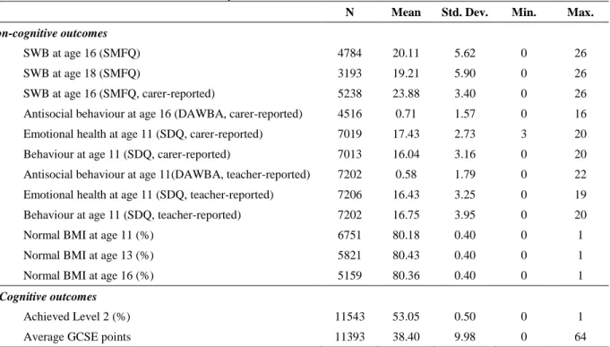
The summary statistics for all of the different child-outcome variables are presented in Appendix Table A1.
3.2 Explanatory Variables
We wish to relate the above dependent variables to the financial resources that were available to the household when the child was growing up. Household income is measured in ALSPAC when the child is aged 3, 4, 7, 8, and 11. The question “On average, about how much is the take
home family income each week (include social benefits etc.)?”is answered using a scale of five
income bands at ages 3, 4, 7 and 8, and ten income bands at age 11. We convert these ALSPAC band values at each wave to income figures using data from the Family Resources Survey (FRS) on the distribution of net household income in the South West region, deflated to 2008 prices. We are careful to match this distribution by year of birth (for 1991 births at age 3, we use the 1994
3 The National Pupil Database (NPD) contains information on pupils’ educational attainments in England, including
test and exam results at different key stages. To date, information on key-stage results is available for each ALSPAC study child at ages 7, 11, 14 and 16. The definition of the different key stages can be found at https://www.gov.uk/national-curriculum/overview.
4https://www.gov.uk/government/uploads/system/uploads/attachment_data/file/517106/Key_stage_4_average_grade
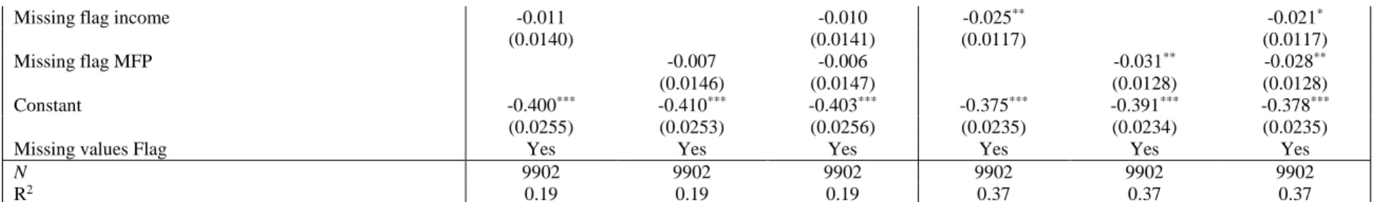
income distribution, but the 1995 income distribution for 1992 births, and so on). The original income bands and the resulting FRS net household income figures appear in Appendix Table A2. As in most survey data, we are confronted with missing values. When the dependent variable is missing, the case is dropped. For missing values on control variables we appeal to the missing indicator approach (as used in Layard et al., 2014). Family income is calculated as the household-level mean over all of the childhood waves in which income information is reported. When all income observations are missing for a given child, we replace the value with the overall sample mean and insert a missing-value flag. About 30% of mothers reported income information in all five waves, while 23% have missing information in all waves. Our final weekly take-home income figure has a mean of £424 and a standard deviation of £150. Family income will be entered in logs in the empirical analyses.
Our second (and more novel) financial variable relates to the major financial problems (MFPs) reported by the child’s mother. The MFP variable may capture financial insecurity over and above traditional income indicators, in the sense that experiencing financial problems is not limited to the poor. Almost every year parents are asked: “Listed below are a number of events
which may have brought changes in your life. Have any of these occurred since your study child’s XXX birthday?”. One of these events is “You had a major financial problem”: see Appendix B1
for further details. We count the number of years from birth to age 11 in which the mother reported a MFP; this question was not asked when the child was aged seven, so that the maximum number of MFPs is ten.
About 37% of mothers answer the MFP question in all ten waves. Another 30% have missing values for one to five waves, 21% have missing values for six to nine waves, while 12% of mothers never replied to this question. When information in some waves is missing, we replace it by the mother’s MFP count in the available waves, multiplied by the ratio of the total number of waves to the observed number of waves.5 When the information is not available in any wave, we replace
the missing value with the total sample mean and introduce a missing-value flag as a right-hand side variable.6
5 With ten potential waves of MFP information, someone who reports eight values (of 0 or 1), will then have their
count over these eight years multiplied by 10/8.
6 We use the same missing-value strategy for the other control variables that are measured similarly (i.e. counting the
number of times during childhood the events occurred), namely number of house moves and the number of years the mother worked.
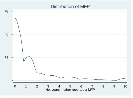
The distribution of MFP after imputation appears in Figure 1. Overall, just under one half of children grew up in households with at least one MFP over the child’s first 11 years, 17% at least two, and 12% at least three, up to a maximum figure of ten. The annual incidence of MFP is correlated with the South-West regional unemployment rate (with a correlation coefficient of 0.16). However, at the household level the correlation between number of MFPs and income is, as expected, negative but not particularly large at -0.16. In particular, financial problems seem to spread up into the middle class. While those in the bottom income quartile (from the average figure over the child’s first 11 years) report an average of 1.7 financial problems, the figures in the second and third income quartile are 1.0 and 0.9 (dropping to 0.5 for the top quartile).
The correlation matrix between all of the dependent and explanatory variables appears in Appendix C. The first column of this matrix reveals the expected correlations with MFPs: they fall with parental education, but rise with job loss, illness, parental separation and income drops. All of these bivariate correlations survive in multivariate regressions.
3.3 Specifications
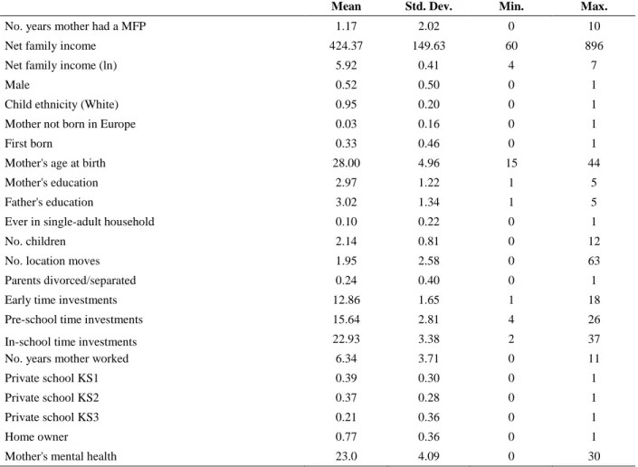
We have three specifications for each child outcome: the first with household income, the second with the number of MFP years, and the third with both together. All regressions include controls for gender, a first-born dummy, mother’s age at the child’s birth, the number of children in the household, single-adult household, parents divorced/separated, parents’ education, child ethnicity, mother born in a non-European country, private school, number of years in which the mother worked, number of house moves, home ownership, and parental time investments (divided into the early, pre-school and in-school periods).7 For all of these other control variables, we replace missing values by the overall sample mean for that variable, and add a missing indicator flag to the regression. The summary statistics of the control variables after imputation, as they appear in the regression analysis, are presented in Appendix Table A3.
Cohort data suffers from attrition, which increases with child age to reach about 40 percent after child age 16. Attrition is more concentrated in lower-income and less-educated families, producing an over-representation of the middle and upper class. This is taken into account in our estimations via inverse probability weighting. We use observable pre-birth information (child’s
7 These investments are measured as the sum of the frequency with which each parent carries out a certain list of
activities with the child, such as bathing her, making things with her; singing to her; reading, playing and active play and preparing food for her. We calculate the average score for the father and the mother.
gender, and mother’s education, age at birth, ethnicity, marital status, employment status, financial problems and mental health) to predict the attrition probability at each child outcome wave, and correct our final estimates using the inverse of the predicted probabilities (1/p) as weights.
To make the results easier to compare across equations, all variables, both dependent and explanatory, are standardised. We also balance the sample within each child-outcome table, so that the estimated coefficients in each column refer to the same children. All of the equations are estimated linearly.
4. Results
This section presents our main results: we broadly show that the correlation between child non-cognitive outcomes and financial problems is larger than that with income (which is mostly insignificant), while for cognitive outcomes the correlations with financial problems and income are of equal size. The full tables of regression coefficients appear in Appendix A (Tables A4 to A7).
4.1 Baseline Results
4.1.1 Child Outcomes, Financial Problems and Family Income
Our main results regarding MFP and income from the specifications that include both at the same time are summarised in Figure 2.
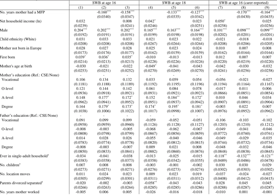
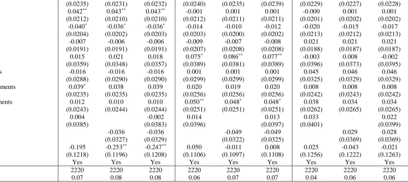
The number of mother’s MFP years is significantly correlated with child-reported SWB at both ages 16 and 18 (Appendix Table A4). The estimated coefficient is remarkably similar for the well-being reported by the child at ages 16 and 18 (columns 1 through 6) and by the carer at age 16 (columns 7 through 9). This similarity helps alleviate any common-method variance concerns regarding MFP and child well-being that are reported by the same person, the carer (although up to fifteen years apart), and thus might be subject to some common reporting style. A one standard-deviation rise in MFP reduces SWB by about 0.15 standard standard-deviations. On the contrary, household real income is only significantly correlated with adolescent SWB in the specification without MFP. Mothers’ financial problems during childhood then have persistent effects on the well-being of their children during adolescence and early adulthood, both as reported by carers and by the
adolescents themselves. This is important, both as a measure of adolescent well-being in itself, and because this well-being is the most important predictor of life satisfaction throughout adult life.
MFP also significantly predicts child antisocial behaviour (reported by the mother in the DAWBA questionnaire at child age 16) in Appendix Table A5.1, columns 1 to 3, with a standardised coefficient of 0.13 that does not change when we include income. The conclusions from the analysis of age 11 externalising SDQ child behaviour in the middle panel are almost identical. Family income is then never significantly correlated with child behaviour once we control for MFP. The right-hand panel of Appendix Table A5.1 turns to child emotional health at age 11 (internalising SDQ): here both MFP and income have separate significant effects.
Appendix Table A5.2 is the teacher-reported version of the child-behaviour analysis in Appendix Table A5.1 (with all outcome variables now being measured at child age 11). The results are qualitatively similar to those for the carer-reported outcomes, but with estimated coefficients on MFP and income that are now insignificant for DAWBA antisocial behaviour at age 11.
The results for our physical health measure, BMI, appear in Appendix Table A6. Only few variables are correlated with child BMI, one of which is mother’s MFP. The effect is negative and significant for BMI at all ages, reducing the probability of normal child BMI by about 0.05 standard deviations. Family income is not significantly correlated with child BMI except at age 11, when it is significant at the 10 percent level.
Last, Appendix Table A7 contains our education results. As in existing UK evidence, family income is positively correlated with child cognitive outcomes. A one standard-deviation rise in income is associated with 0.04 standard-deviation higher average GCSE points at age 16. This effect size is somewhat higher than that of MFP, which is however related in its own right to child GCSE points. At the upper tail of the GCSE distribution (the probability of achieving Level 2), MFP and income attract similar significant estimated coefficients. The MFP coefficients regarding education are in general smaller in size than those for the various non-cognitive outcomes discussed above. One reason why family income is less significant for achieving Level 2 is that one of our controls, home ownership, is the strongest predictor of both of the educational outcomes. Section 4.2.6 describes how all of our estimation results are affected by dropping home ownership as a control variable. Here excluding home ownership produces an estimated family-income coefficient of 0.04 for achieving Level 2, with the MFP coefficient being unaffected.
The principal conclusion from these regression tables, as summarised in Figure 2, is that children growing up in families where the mother reports having financial problems have significantly worse cognitive and non-cognitive outcomes, controlling for family income. MFP is a stronger predictor of children’s non-cognitive outcomes than is family income (the average standardised absolute-value MFP coefficient for the non-cognitive outcomes being 0.10), with family income being insignificant for most child non-cognitive outcomes. On the contrary, both family income and MFP are significantly correlated with the child’s cognitive outcomes at age 16.
4.1.2 The other correlates of child outcomes
Gender is the strongest correlate of children’s SWB: boys have higher SWB by between 0.10 and 0.20 standard-deviation points, in line with existing work on adolescent mental health (e.g. Duncan et al., 1985, and Nolen-Hoeksema and Girgus, 1994) where girls report more dissatisfaction and psychological problems than do boys (although adult women report both higher life satisfaction and higher stress scores than do men: Nolen-Hoeksema and Rusting, 1999). Only few other variables are significantly correlated with child SWB. While it is commonplace that parents’ education affects child cognitive development, we here find only mostly insignificant SWB effects of mother’s education and no effect of father’s education. Being first born attracts a positive coefficient for child-reported SWB, as does home ownership. Last, growing up in a single-parent household reduces carer-reported SWB at age 16, but not child-reported SWB.
There is no gender effect on antisocial behaviour at age 16, in contrast to some existing work suggesting that boys are worse offenders than girls (see Gregg and Machin, 2000, for contacts with the police), but evidence that boys are worse-behaved at age 11. This is consistent with work showing that the behavioural gender gap falls with age (Cohen et al., 1993). Parental separation is associated with more antisocial behaviour, while this latter falls with father’s (but not mother’s) education. Pre-school time investments and private school at KS3 (age 14) are associated with better child behaviour.
We find no gender effect on emotional health at age 11. Mother’s education has a positive effect on child emotional health at age 11. The presence of other children in the household improves both emotional health and behaviour, as do time investments and mother’s years of work. More variables are significant in the teacher-reported version of the behaviour and emotional health table (Table A5.2). Boys again behave worse and (to a lesser extent) have worse emotional health. White children also have lower emotional health. The first-born have better behaviour but
worse emotional health. Home ownership and parental education are associated with better teacher-reported outcomes for almost all measures, while parental separation produces worse outcomes. As for the carer-reported outcomes, mother’s employment is positively related to child emotional health but not behaviour.
Apart from MFP, only few variables are correlated with BMI and we in particular find no gender effect. We will consider some alternative physical health measures in Section 4.2.5 below. Home ownership is amongst the strongest predictors of cognitive outcomes, with an effect size of about 0.12 standard deviations. Girls, the first-born, and those with older mothers and better-educated parents record better educational performance; the number of siblings and parental separation are associated with lower test scores.
4.2 Extensions to the Baseline Results
4.2.1 Channels
The family-process channel in Section 2 emphasised the mediating role of parental stress. One aspect of this stress (but far from the only one) is mother’s mental health. In ALSPAC this latter is measured by the Edinburgh Post-natal Depression Scale, developed by Cox et al. (1987). This is composed of ten items referring to the feelings of the mother over the past week (see Appendix B6). The score ranges from 0 to 30, and is reversed so that higher values indicate better mental health. Although this measure was developed for use with puerperal women, none of the items is specifically related to the post-natal experience, and it has been validated for use during pregnancy, post-partum and early parenthood. Mother’s mental health is measured at child ages of 8, 21, 33, 61, 73, 97 and 134 months.
It is commonplace in the existing literature to find that low income, debt and financial insecurity among adults reduce their subjective well-being. Some examples are Clark et al. (2016) regarding poverty, Brown et al. (2005) and Gathergood (2012) for debt, Kopasker et al. (2016) with respect to insecurity, and Deaton (2012) and Wahlbeck and McDaid (2012) for financial crises. We do indeed find a correlation in ALSPAC data between mother’s mental health and both MFP and income.
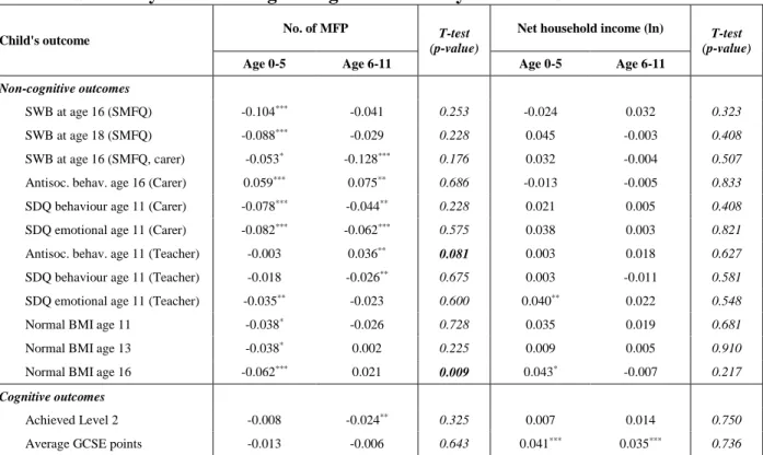
When we add mother’s mental health to the regressions described in Section 4.1.1 above, we find that this plays a significant mediating role for most non-cognitive outcomes, as summarised in Table 1. The first two columns show our baseline estimated coefficient (those in Figure 2) on
income and financial problems; columns 3 and 4 then present these same coefficients controlling for mother’s mental health, with the last two columns showing the percentage change in the two estimated coefficients.
Children whose mothers have better mental health have better outcomes on all measures bar BMI, with the correlation with the cognitive outcomes being the smallest. Controlling for mother’s mental health reduces the MFP coefficient by about one-quarter to one-half for well-being, behaviour and emotional health, although the estimated MFP coefficient mostly continues to be negative and significant in its own right. By way of contrast, mother’s mental health makes little difference to the estimated MFP coefficients for child BMI and education. Mediation via mother’s mental health is then more salient for non-cognitive outcomes.8
There is more than one interpretation here. Perhaps the most obvious is that of a mediator: income and financial problems affect mother’s mental health, which in turn affects child outcomes. In this light, one quarter to one half of the effect of MFP on well-being, behaviour and emotional health works via mother’s distress (from column 5 of Table 1). Alternatively, we could think that reported financial problems are themselves partly determined by mother’s mental health, in the sense that more “anxious” mothers are more likely to report problems. In this respect the emphasis is now more on the third column of the table, showing that MFP continues to have an effect conditional on mother’s mental health.
There are a number of other possible mediators via which MFP could affect child outcomes. Four of these are controlled for in our standard regressions: living in a single-adult household, parental separation, parental time investments and mother’s work. To evaluate mediation, we have re-run the regressions in column 3 of each panel of the regression tables in the Appendix excluding each of these variables in turn. This exercise produces only very marginal changes in the estimated MFP coefficients: separation, single parenthood, time investments and mother’s work are not behind the effect of MFP on child and adolescent outcomes.
Last, we can tackle this issue in the opposite direction, and add more control variables that may be behind MFP to the baseline regression. Following the significant bivariate correlations in Appendix C, we thus add controls for the experience of mother’s illness, mother’s job loss and
8 The mediating effect of mother’s mental health on the estimated income coefficients in the last column is perhaps of
less interest, because only few of the latter were significant to start with (see Figure 2). The inclusion of mother’s mental health has only little effect on the significant income coefficients.
partner’s job loss over the child’s first eleven years (calculated in the same way as our variable of experience of MFP). The addition of these three new variables reduced the coefficient on MFP as expected, but only by around 10% for most non-cognitive outcomes. The reduction in the estimated MFP coefficient for cognitive outcomes was somewhat larger: parental job loss and illness may play a more important role for adolescent exam results than they do for non-cognitive outcomes. In general, there is much more behind MFP (in terms of its consequences on adolescent outcomes) than is picked up by this array of early-life events.
4.2.2 Early versus late childhood
The existing literature on the importance of early vs. late childhood has produced ambiguous results: see, for example, Duncan and Brooks-Gunn (1997), Duncan et al. (1998), Guo (1998), Haveman et al. (1991), Heckman (2006) and Wagmiller et al. (2006). Early-childhood deprivation can be argued to affect the development of basic cognitive skills, feeding through to later achievements; alternatively, children may be more aware of economic disadvantage in later childhood, reducing their self-esteem and thus their outcomes (see, for example, Ogbu, 1978, and Mickelson, 1990).
We here separately estimate the effect of economic resources for early and late childhood (ages 0 to 5 and 6 to 11 respectively). Table 2 summarises the results, and shows the t-statistics from the tests of coefficient equality across childhood ages (the full table of results appears in Appendix Table A8). There are almost never different estimated MFP coefficients in early and late childhood in Table 2. The exception is child BMI, where early-childhood financial problems lead to worse BMI outcomes but those in later childhood do not (perhaps reflecting that children eat at home more often before the start of compulsory schooling). This overall pattern is repeated in regressions that condition on mother’s mental health (results available on request). The effect of income in the two childhood periods does not differ statistically for any outcome.9
9 We also experimented with decay functions, weighting MFPs at the different child ages by the ratio of child age at
MFP report to child age at outcome, which gives more weight to more recent MFPs, or by the complement of this expression, giving more weight to earlier MFPs. The fit of the regressions (as measured by the R-squared) barely changed.
4.2.3 Sub-group analyses
The pattern of our results is remarkably similar when we estimate boys’ and girls’ outcomes separately: the differences refer to income and cognitive outcomes, and MFPs and teacher-reported behaviour at age 11, both of which are only correlated for boys. This pattern of results chimes with the gender difference in cognitive outcomes and behaviour following family disadvantage in Autor
et al. (2016), but no sex differences in the way in which negative cognitive style, depression and
rumination are correlated with an index of negative or stressful life events that typically occur during adolescence in Hamilton et al. (2015). There are also no striking differences for children in above- and below-median income households (where income refers to the average household figure over the child’s first eleven years).10
4.2.4 Non-linearities
To see whether low values of MFP are unimportant, we cut the non-zero MFP distribution at its median and created two dummy variables. From Figure 1, this median is at a value of around 1.7. We would in general expect the estimated coefficient for below-median MFPs to be smaller than that on above-median MFPs. For a number of outcomes we find that the former is insignificant. This is in particular the case for child-reported well-being, and both cognitive outcomes. For these variables, a small number of MFPs does not matter: the overall negative MFP coefficient listed in Table 1 rather comes from those children whose mothers experienced repeated financial problems.
4.2.5 Alternative physical health measures
Physical health above was measured a dummy variable for child BMI being between the 5th
and 85th percentiles by age and sex. We also ran all of our analyses considering only the upper tail of the BMI distribution, i.e. a dummy for being above the 85th percentile of the specific gender-age distribution. This made no difference to the results.
We also have information on a number of child physical health symptoms at age 11 (such as stomach ache, arms/legs ache, cough at night, infection and asthma). We construct a dummy variable for the total number of symptoms being in the top 40% of the distribution (as in Propper
10 Four out of 28 estimated MFP and income coefficients are significantly different between above- and below-median
et al., 2007), and also look at the total number of symptoms. Last, we have information on the
general health of the child as assessed by the mother, and create a dummy for the child being anything other than very healthy. The results for both of the symptoms variables mirror those for BMI: the number of major financial problems attracts a positive estimated coefficient that is significant at the one per cent level while that on income is insignificant.11 Regarding child overall
health at age 11, both MFP and income attract significant estimated coefficients of roughly equal size.
4.2.6 Income and Wealth
All of our results above concerning income and MFP come from regressions which condition on a range of control variables, including home ownership. This latter is often considered as a measure of wealth. To check whether any correlation between wealth and income (or indeed between wealth and MFP) is affecting our conclusions, we have re-run our regressions dropping home ownership. This makes almost no difference to the estimated MFP coefficients that are summarised in Table 1. It also does not affect our conclusions regarding the correlation between income and child non-cognitive outcomes. Where it does make a difference is for income and cognitive outcomes. Home ownership is one of the strongest predictors of both of our educational outcomes (see Table 7A), and its exclusion from the child-education regressions leads to estimated income coefficients that almost double in size relative to those in Table 1.
4.2.7 Issues in Imputation
Both the income and financial-problems variables in the regressions contain some imputed values. The distribution of financial problems including imputed values in Figure 1 shows a slight uptick at the maximum value of 10. This almost never reflects a respondent reporting problems ten times, but rather someone who is interviewed four times (say), reports a financial problem each time, and then has an imputed value of 10 (as 4 x 10/4). All of our results are robust to dropping this maximum category in our adolescent-outcome regressions.
Along the same lines, it might be thought that imputing missing values produces an over-estimation of the incidence of financial problems. As an experiment, we instead replace all missing
11 Janssen and Sandner (2016) exploit information on a German welfare reform, and also find no effect of household
values by zero, including the financial-problems score of those who are missing at every wave with respect to this variable: this undoubtedly produces an under-estimate of incidence. The “missing as zero” estimation results reveal smaller estimated coefficients on financial problems, all of which remain significant and mostly larger than those on income (which hardly change).
Our approach to missing income information was to calculate the average of the five reported values over childhood. If fewer than five were reported, we took the average over the reported figures only (which amounts to replacing the missing information by the individual-level mean). If all five were missing, we replaced by the sample mean and created a missing income flag. Around 23% of observations were missing income at all waves. We first check that our results remain unchanged when we simply drop this 23% group. This produces estimated coefficients on income that are sometimes larger than those in our main results, but broadly does not change their pattern. Notably the income coefficients for cognitive outcomes are now considerably larger than those on financial problems (although all estimated coefficients remain significant at the five per cent level or better).
We have also changed the imputation approach for all variables from missing indicator to multiple imputation.12 The estimated results again remain similar (although, as above, the estimated income coefficients in the cognitive-outcome regressions are notably larger).
4.2.8 Falls in income and major financial problems
Our main results refer to financial problems and the level of household income, and we in general underline the importance of the former over the latter (at least for the non-cognitive outcomes). Although the level of income and MFP are only correlated at 0.16, we might imagine that falls in income are a key cause of MFP. Due to the banded (and infrequent) nature of the ALSPAC income variable, we cannot observe these income drops directly. However, we do have annual information on whether the mother reported a fall in income over the past year. We count the number of years with an income drop. This count is correlated with MFP at 0.5.
Regressions with income, MFP and income drops produce estimated coefficients on the first two variables that are very similar to those summarised in Figure 2. For the non-cognitive
12 Multiple imputation was performed using chained equations with ten imputations, assuming that missing
observations are missing at random (MAR) given the known characteristics of the individuals for which observations are missing. Estimates from the ten imputed datasets are then combined using Rubin’s rule. This approach has already been used in other papers based on ALSPAC (see e.g. Washbroook et al., 2014).
outcomes, income remains significant only for the two internalising SDQ variables at age 11, while MFP remains significant for almost all non-cognitive outcomes with estimated coefficients that are attenuated by only 10-20%. The results for the cognitive outcomes are not at all affected. The income-drop variable itself is significantly correlated with all three well-being variables, the carer and teacher-reported anti-social behaviour variables, and carer-reported child behaviour and emotional health. The estimated coefficient on the (standardised) income-drop variable is always smaller than that on standardised MFP.
5. Conclusion
Financial insecurity and stress are central determinants of well-being. We here use large-scale and long-run birth cohort data to make two central contributions in this context. We first extend the typical contemporaneous analysis by relating family financial insecurity experienced during childhood to a range of cognitive and non-cognitive outcomes experienced during the intermediate period of adolescence. Second, we do not limit ourselves to income as the single measure of financial stress, but also consider the incidence of financial problems as reported by the mother. Our broad premise is that income alone may be an insufficient indicator of the economic resources and demands placed on them that jointly determine financial stress.
This premise is borne out in the empirical results. All of our adolescent non-cognitive outcomes are significantly correlated with childhood financial problems, but few are correlated with childhood income. The adolescent cognitive outcomes are correlated with both financial problems and income. While we then agree with Duncan and Brooks-Gunn (1997) that non-cognitive outcomes are less sensitive to family income than are non-cognitive outcomes, we notably find exactly the opposite ordering with respect to family financial problems.
Our results underline that childhood financial problems are significantly correlated with most adolescent outcomes, even after controlling for family income. This correlation does not seem to be subject to contamination by mood, as the reports of financial problems and child outcomes are separated by a period of up to 17 years. In addition, we find correlations not only with mother’s reports of adolescent outcomes but also with those reported by the adolescent him/herself and by teachers.
In the recent Great Recession, the types of financial problems that we analyse here have arguably become more widespread than low income, and have extended to hit the middle-class as
well (as highlighted, for example, by Gauthier and Furstenberg, 2010, in relation to families with children). The Federal Reserve’s Report on the Economic Well-Being of U.S. Households in 2014 highlighted that 24% of individuals had experienced some form of financial hardship over the past year, and 47% could not cover an unexpected expense of $400. More recently, a December 2015 survey by Bankrate13 found that 63% of Americans have no emergency savings for a $1000
emergency-room visit or a $500 car repair, and a July 2016 UK survey by the housing charity Shelter14 that 37% of working families would be unable to cover their housing expenses were one
of the partners to lose their jobs. This widespread financial insecurity undoubtedly has sharp effects on the well-being of the individuals concerned; our work here also suggests that it may cast a long shadow over the outcomes of their children many years in the future.
13 Bankrate: http://www.bankrate.com/finance/consumer-index/money-pulse-1215.aspx. 14 Shelter: http://www.bbc.com/news/uk-england-37017254.
References
Acemoglu, D., Pischke, J.-S., 2001. Changes in the wage structure, family income, and children's education. European Economic Review 45, 890-904.
Autor, D., Figlio, D., Karbownik, K., Roth, J., Wasserman, M., 2016. Family Disadvantage and the Gender Gap in Behavioral and Educational Outcomes. MIT, Working Paper.
Axinn, W., Duncan, G.J., Thornton, A., 1997. The effects of parents’ income, wealth, and attitudes on children’s completed schooling and self-esteem.In G.J.Duncan, J.Brooks-Gunn (Eds.),
Consequences of growing up poor. New York: Russell Sage Foundation.
Becker, G.S., 1981. A Treatise on the Family. Cambridge: Harvard University Press.
Becker, G.S., Tomes, N., 1986. Human capital and the rise and fall of families. Journal of Labor
Economics 4, S1-S39.
Becker, G.S., Tomes, N., 1994. Human capital and the rise and fall of families. Human Capital: A Theoretical and Empirical Analysis with Special Reference to Education (3rd Edition). Chicago: University of Chicago Press, 257-298.
Black, S.E., Devereux, P.J., Salvanes, K.G., 2005. The more the merrier? The effect of family size and birth order on children's education. Quarterly Journal of Economics 120, 669-700. Blanden, J., Gregg, P., 2004. Family income and educational attainment: a review of approaches
and evidence for Britain. Oxford Review of Economic Policy 20, 245-263.
Blau, D.M., 1999. The effect of income on child development. Review of Economics and Statistics 81, 261-276.
Bolger, K.E., Patterson, C.J., Thompson, W.W., Kupersmidt, J.B., 1995. Psychosocial adjustment among children experiencing persistent and intermittent family economic hardship. Child
Development 66, 1107-1129.
Bossert, W., D'Ambrosio, C., 2013. Measuring Economic Insecurity. International Economic
Review 54, 1017-1030.
Brown, S., Taylor, K., Wheatley-Price, S., 2005. Debt and distress: Evaluating the psychological cost of credit. Journal of Economic Psychology 26, 642-663.
Case, A., Paxson, C., 2002. Parental behavior and child health. Health Affairs 21, 164-178. Clark, A.E., D'Ambrosio, C., Ghislandi, S., 2016. Adaptation to Poverty in Long-Run Panel Data.
Review of Economics and Statistics 98, 591-600.
Clark, A.E., Flèche, S., Layard, R., Powdthavee, N., Ward, G., 2018. The Origins of Happiness:
Conger, R.D., Conger, K.J., Martin, M.J., 2010. Socioeconomic Status, Family Processes,and Individual Development. Journal of Marriage and the Family 72, 685-704.
Cohen, P., Cohen, J., Kasen, S., Velez, C.N., Hartmark, C., Johnson, J., Rojas, M., Brook, J., Streuning, E., 1993. An Epidemiological Study of Disorders in Late Childhood and Adolescence I. Age- and Gender- Specific Prevalence. Journal of Child Psychology and
Psychiatry 34, 851-867.
Cox, J.L., Holden, J.M., Sagovsky, R., 1987. Detection of postnatal depression. Development of the 10-item Edinburgh Postnatal Depression Scale. British Journal of Psychiatry 150, 782-786.
Currie, J., Stabile, M., 2002. Socioeconomic status and health: why is the relationship stronger for older children? National Bureau of Economic Research.
Deaton, A., 2012. The financial crisis and the well-being of Americans. Oxford Economic Papers 64, 1-26.
Duncan, G.J., Brooks-Gunn, J., 1997. Consequences of growing up poor. New York: Russell Sage Foundation.
Duncan, P.D., Ritter, P.L., Dornbusch, S.M., Gross, R.T., Carlsmith, J.M., 1985. The effects of pubertal timing on body image, school behavior, and deviance. Journal of Youth and
Adolescence 14, 227-235.
Duncan, G.J., Yeung, W.J., Brooks-Gunn, J., Smith, J.R., 1998. How much does childhood poverty affect the life chances of children? American Sociological Review 63, 406-423.
Elder, J., 1997. Children of the Great Depression. 25th Anniversary Edition. Boulder, CO: Westview Press.
Ermisch, J., Francesconi, M., 2001. Family matters: Impacts of family background on educational attainments. Economica 68, 137-156.
Evans, G., Cassells, R., 2014. Childhood Poverty, Cumulative Risk Exposure, and Mental Health in Emerging Adults. Clinical Psychological Science, 2, 287-296.
Feinstein, L., 2000. The relative economic importance of academic, psychological and behavioural
attributes developed on childhood. Centre for Economic Performance, London School of
Economics and Political Science.
Flèche, S., Lekfuangfu, W., Clark, A.E., 2017. The long-lasting effects of childhood on adult wellbeing: Evidence from British cohort data. CEP Discussion Paper No. 1493.
Ford, T., Goodman, R., Meltzer, H., 2004. The relative importance of child, family, school and neighbourhood correlates of childhood psychiatric disorder. Social Psychiatry and Psychiatric
Gathergood, J., 2012. Debt and Depression: Causal Links and Social Norm Effects. Economic
Journal 122, 1094-1114.
Gauthier, A.H., Furstenberg, F.F., 2010. The experience of financial strain among families with children in the United States. National Center for Family & Marriage Research, Working Paper WP-10-17.
Goodman, R., Lamping, D. L., Ploubidis, G. B., 2010. When to use broader internalising and externalising subscales instead of the hypothesised five subscales on the Strengths and Difficulties Questionnaire (SDQ): data from British parents, teachers and children. Journal of
Abnormal Child Psychology 38, 1179-1191.
Gregg, P., Machin, S., 2000. Child development and success or failure in the youth labor market. NBER Comparative Labour Market Series. Chicago: University of Chicago Press, 247-288. Guo, G., 1998. The timing of the influences of cumulative poverty on children's cognitive ability
and achievement. Social Forces 77, 257-287.
Guo, G., Harris, K.M., 2000. The mechanisms mediating the effects of poverty on children’s intellectual development. Demography 37, 431-447.
Hamilton, J., Stange, J., Abramson, L., Alloy, L., 2015. Stress and the Development of Cognitive Vulnerabilities to Depression Explain Sex Differences in Depressive Symptoms During Adolescence. Clinical Psychological Science 3, 702-714.
Hardy, B.L., 2014. Childhood income volatility and adult outcomes. Demography 51, 1641-1665. Haveman, R., Wolfe, B., 1995. The determinants of children's attainments: A review of methods
and findings. Journal of Economic Literature 33, 1829-1878.
Haveman, R., Wolfe, B., Spaulding, J., 1991. Childhood events and circumstances influencing high school completion. Demography 28, 133-157.
Heckman, J.J., 2006. Skill formation and the economics of investing in disadvantaged children.
Science 312, 1900-1902.
Heckman, J.J., Stixrud, J., Urzua, S., 2006. The effects of cognitive and noncognitive abilities on labor market outcomes and social behavior. Journal of Labor Economics 24, 411-82.
Janssen, S. and Sandner, M., 2016. Household Income and Infant Health. Evidence from a Welfare Benefits Reform. IAB Nuremberg, mimeo.
Kalil, A., 2013. Effects of the Great Recession on Child Development. Annals AAPSS 650, 232-249.
Kim, Y., Sherraden, M., 2011. Do parental assets matter for children's educational attainment?: Evidence from mediation tests. Children and Youth Services Review 33, 969-979.