HAL Id: hal-00394171
https://hal.archives-ouvertes.fr/hal-00394171
Submitted on 10 Jun 2009
HAL is a multi-disciplinary open access
archive for the deposit and dissemination of
sci-entific research documents, whether they are
pub-lished or not. The documents may come from
teaching and research institutions in France or
L’archive ouverte pluridisciplinaire HAL, est
destinée au dépôt et à la diffusion de documents
scientifiques de niveau recherche, publiés ou non,
émanant des établissements d’enseignement et de
recherche français ou étrangers, des laboratoires
Regularization of inverse problems with adaptive
discrepancy terms: application to multispectral data
Sandrine Anthoine
To cite this version:
Sandrine Anthoine. Regularization of inverse problems with adaptive discrepancy terms:
applica-tion to multispectral data. SPIE Wavelets XII, Aug 2008, San Diego, United States. pp.670110,
�10.1117/12.733643�. �hal-00394171�
Regularization of inverse problems with adaptive discrepancy terms;
application to multispectral data
Sandrine Anthoine
I3S, Université de Nice Sophia-Antipolis, CNRS;
2000 route des Lucioles, 06903 Sophia-Antipolis Cedex, France
ABSTRACT
In this paper, a general framework for the inversion of a linear operator in the case where one seeks several components from several observations is presented. The estimation is done by minimizing a functional balancing discrepancy terms by regularization terms. The regularization terms are adapted norms that enforce the desired properties of each component.
The main focus of this paper is the definition of the discrepancy terms. Classically, these are quadratic. We present novel discrepancy terms adapt to the observations. They rely on adaptive projections that emphasize important information in the observations. Iterative algorithms to minimize the functionals with adaptive discrepancy terms are derived and their convergence and stability is studied.
The methods obtained are compared for the problem of reconstruction of astrophysical maps from multifrequency observations of the Cosmic Microwave Background. We show the added flexibility provided by the adaptive discrepancy terms.
Keywords: inverse problems, iterative algorithm, adaptive discrepancy terms, wavelets, multispectral astrophysical data.
1. INTRODUCTION
In a general inverse problem, the goal is to estimate an objectF from an observation G where G=T (F ) (for example looking for the original from a blurred picture). Here we assume that T , the linear operator modeling the observation process, is known. Even so, the problem is often ill-posed and therefore needs to be “regularized”. This amounts to finding an estimate eF which has the two following properties:
1. eF should generate observations close to the data (T ( eF ) ≈ G).
2. eF should have properties we expect from a priori knowledge. (In the example of the blurred picture, we expect eF to have sharp features.)
A number of classical methods for solving inverse problems try to balance the fitness to the data (T ( eF ) ≈ G), measured by a discrepancy termJdisc, with the regularity of the solution (i.e. the properties of eF ), measured a regularization term Jreg,
by minimizing a cost functional of the type:
J(F ) = Jdisc¡T (F ), G¢+ αJreg(F ) (1)
The main focus of this paper is the definition of the discrepancy term. Generally, this term is chosen to be theL2
norm of the residualG − T (F ) i.e. Jdisc(T (F ), G) = ||G − T (F )||2L2 =
R
|G(x) − T (F (x))|2dx or a similar quadratic
norm. Such a term treats uniformly all the elements inG (for example all the pixels in an image). However, it is clear that some part ofG carry more information than others and should therefore be treated differently. For example, in a blurred picture, one is usually more interested in recovering well the face of a person than the uniform part of the sky. A simple quadratic norm is not able to identify such important features and thus may be improved. J.-L. Starck and co-authors in1present an iterative algorithm that focuses on these important features in blurred astrophysical images by introducing
projections on the “multiresolution support”. These are projections on a subspace defined by the wavelet transform of the observations. They are adaptive and allow to consider only important features of the data and discard the noise in the case of deconvolution of astrophysical data presented in1. Following this idea, we propose the use of general projections to
define adaptive discrepancy measures. The idea is that the image space of the projection defines important features in the observation - these should be well predicted by the estimate ofF - while the kernel of the projection defines information that is less important or even not relevant (for example noise in the observation). Using the mathematical framework introduced in2, we study the mathematical properties of the resulting algorithms. We show that convergence is guaranteed and that stability holds in a certain sense. However we point out that the use of projections may result in a loss of information that prevents to recover some parts of the data. We show that this can be remedied by introducing the notion of “relaxed projection”, which consists in only down-weighting the importance of the non-feature space instead of cancelling it.
After the present introduction, this paper is organized as follows. In the second section we introduce the notations as well as the variational framework we use, i.e. the class of functionals we seek to minimize as well as an iterative algorithm to solve the minimization. The third section concerns the generalization of discrepancy terms via the use of projections and its mathematical study. The potential loss of information induced by the projections is remedied in section four by the introduction of relaxed projections. Finally, section five is devoted to the application of the resulting algorithms to the estimation of astrophysical maps from multifrequency observations.
2. A CLASS OF VARIATIONAL FUNCTIONAL TO REGULARIZE INVERSE PROBLEMS
2.1 Notations
2.1.1 Inverse problem with several objects and observations
The most general problem we will consider is the case where we seekM objects or components f1, .., fM fromL
observa-tionsg1, ..., gL. In the case of the estimation of astrophysical maps from multifrequency observations, each objectfiis the
map of an astrophysical phenomena (ex: the map of galaxy clusters) and eachglis an observation of the sky at wavelength
νl.
We make the following assumptions: • Each object belongs to a Hilbert space Hi
m:∀m = 1..M, fm∈ Him.
• Each observation belongs to a Hilbert space Ho
l:∀l = 1..L, gl∈ Hlo.
• We know the linear bounded operators Tm,l: Him→ Hol
such that the model for the observations is linear with additive noise: ∀l = 1..L, gl=
M
X
m=1
Tm,lfm+ nl (2)
wherenlare noise terms.
To estimate the objectsf1, .., fM fromg1, ..., gL, we will minimize functionals composed of a sum of discrepancy
terms (one per observation) and regularization terms (one per component) such as: J(f1, f2, . . . , fM) = L X l=1 ρl ° ° °( M X m=1 Tm,lfm− gl) ° ° ° 2 Ho l + M X m=1 γm|||fm|||Xm; (3)
where theγmandρlare strictly positive scalars and the “norms”|||.|||Xm are of the form:
|||f |||Xm = X λ∈Λ wλm| hf, ϕmλi |p m (4) where for allm, ϕm= {ϕm
λ}λ∈Λ is a generating family ofHim,wλm> 0 and 1 ≤ pm≤ 2.
The discrepancy terms (first sum in Eq.(3)) are classical quadratic terms. The particular form of the|||.|||Xm is chosen
so that one can adapt the regularization terms (second sum in Eq.(3)) to the properties of each object. Indeed, for eachm, one chooses the decomposition system ϕm= {ϕm
λ}λ∈Λ on which to measure the smoothness of the mth object, as well as
the type oflpmeasure and weights needed. This gives a large panel of available smoothness measures that can fit various
kind of data. For example, the Cosmic Microwave Background signal, which is the relic radiation of our Universe, is well modeled by a Gaussian process with known spectral powerP . The Gaussianity leads to a quadratic measure, while the power spectrum can be enforced in Fourier space. Therefore, an adapted measure isPkP (k)−1| hf, exp(−2πjk)i |2. As
for galaxy clusters, these being rare, small and intense objects, the wavelet transform of such a map is sparse (only a few coefficients of large amplitude). Therefore, an adapted term is thel1norm of its wavelet coefficients:Pj,k| hf, ψj,ki |.
2.1.2 Simplifying notations: case of one object and observation
One can simplify greatly the notations by ”vectorizing” the previous problem as follows:
find one objectF = (f1, f2, . . . , fM)T from one observationG = (g1, g2, . . . , gL)T, knowingT = {Tm,l}m,l, the linear
operator such that:
G = T F + N (5)
The functional in Eq.(3) is then:
J(F ) =°°T F − G°°2Ho+ γ|||F ||| ; (6)
where the norm in Hilbert spaceHois the weighted Euclidean norm: °°G°°2 Ho = PL l=1ρl ° °Gl ° °2 Ho l
and|||F ||| is the mixed norm|||F ||| =PMm=1γm|||fm|||Xm =
PM
m=1γmPλ∈Λwmλ| hf, ϕmλi |p
m
. Written this way, Eq.(6) is very close to Eq.(3) with M=L=1, which reads:.
J(f ) =°°T f − g°°2Ho+ γ|||f ||| = ° °T f − g°°2 Ho + γ X λ∈Λ wλ| hf, ϕλi |p (7)
It is true that the weighted norm induced onHomakes it a standard Hilbert space, hence the discrepancy terms do match
perfectly. But the regularization terms do not match: for M=1, we get in Eq. (7) a simplelpsum (with a single exponent
p), which is not true for M>1.
However, the minimization of Eq.(6) can be done by slightly modifying the iterative algorithm that we use for Eq.(7) and moreover, the proofs of convergence and stability carry to this more complicated case (see3 for details). Since in this
paper we are concerned with modifying the discrepancy term, we will only present the theory with a simple regularization term as in Eq.(7) to alleviate the notations, keeping in mind the mixed regularization terms for the application.
Note that we will use the following notations: • the sequence of weight is: w = {wλ}λ∈Λ.
• the functional in Eq.(7) is Jγ,w,p(f ) =
°
°T f − g°°2Ho + γ
P
λ∈Λwλ| hf, ϕλi |p.
• the scalar product is: fλ= hf, ϕλi.
• we call ||| · |||w,p–norm the quantity:Pλ∈Λwλ| h· , ϕλi |p.
2.2 A class of functionals and the study of their minimization
In this section, we summarize the findings in2, which concern the minimization of Eq.(7), i.e. of the functional J γ,w,p.
2.2.1 Iterative algorithm
The authors propose the following iterative algorithm to obtain a minimizer:
ALGORITHM2.1. ½
f0 arbitrary
fn = S
γw,p¡fn−1+ T∗(g − T fn−1)¢, n ≥ 1
At each iteration, one computes the Landweber iteratefn−1+ T∗(g − T fn−1) and modifies it with the S
γw,pfunction.
The Sγw,ptreats independently each coefficient of the argumenth on the decomposition system ϕ= {ϕλ}λ∈Λ:
Sw,p(h) =
X
λ
Swλ,p(hλ)ϕλ , (8)
with the functionsSw,pfrom R to itself given by
Sw,p(x) def = ³x + wp 2 sign(x) |x| p−1´−1 , for 1 ≤ p ≤ 2, (9) where(.)−1denotes the inverse so that∀x, S
w,p(x + wp2 sign(x) |x|p−1) = x.
In particular, forp = 1, Sw,1is the soft-thresholding operator: Sw,1(x) = sign(x)(|x| − w/2)+
2.2.2 Convergence and stability
The two following theorems summarize the findings presented in2. The first theorem states that the iterative algorithm 2.1
converges strongly in the norm associated in the Hilbert spaceHifor any initial guessf0.
THEOREM2.2 (CONVERGENCE). LetT be a bounded linear operator from HitoHo, with|||T ||| < 1. Take p ∈ [1, 2], and
let Sw,pbe the shrinkage operator defined by(8), where the sequence w = {wλ}λ∈Λ is such that there exists a constant
c > 0 such that ∀λ ∈ Λ : wλ≥ c. Then the sequence of iterates
fn= Sγw,p¡fn−1+ T∗(g − T fn−1)¢, n = 1, 2, . . . ,
withf0arbitrarily chosen inHi, converges strongly to a minimizer of the functional J γ,w,p.
If the minimizerf⋆of J
γ,w,pis unique, (which is guaranteed e.g. byp > 1 or ker(T ) = {0}), then every sequence of
iteratesfnconverges strongly tof⋆, regardless of the choice off0.
The second theorem is concerned with the stability of the method. It gives sufficient conditions to ensure that the estimate recovered from a perturbed observation,g = T f0+ e, will approximate the object f0as the amplitude of the
perturbationkekHogoes to0.
THEOREM2.3 (STABILITY). Assume thatT is a bounded operator from HitoHowith|||T ||| < 1, that γ > 0, 1 ≤ p ≤ 2
and that the entries in the sequence w= {wλ}λ∈Λare bounded below byc > 0.
Assume that eitherp > 1 or ker(T ) = {0}. For any g ∈ Hoand anyγ > 0, define fγ,w,p;g⋆ to be the minimizer of
Jγ,w,pwith observationg. If γ = γ(²) satisfies lim
²→0γ(²) = 0 and ²→0lim
²2
γ(²) = 0 , (10)
then we have, for anyfo∈ Hi,
lim ²→0 " sup kg−T fokHo≤² kfγ(²),w,p;g⋆ − f†kHi # = 0 , (11)
wheref†is the unique element of minimum||| · |||
w,p–norm in the setSfo = {f ; T f = T fo}.
Note that in particular whenT is invertible, f†= f which means that Algorithm 2.1 provides a stable inversion. So far, we have a convergent and regularizing iterative algorithm that converges to a minimizer of the functional Jγ,w,p.
Such a minimizer is an estimate of the objectf that compromises between generating an observation close to the data g in a quadratic sense and having the smallest||| · |||w,p–norm. Note the the design of the||| · |||w,p–norm is such that it will
preserve or enhance desirable properties off . The quadratic discrepancy term in Jγ,w,pis devoid of such considerations
and therefore does not enhance more important features that should be matched in the observations. In the rest of this paper, we will present adaptive discrepancy terms that aim at fixing this point.
3. ADAPTIVE DISCREPANCY TERMS (I): USING PROJECTIONS
3.1 An Algorithm using Adaptive Projections
3.1.1 Original idea
In1, the authors are concerned with the deconvolution of an astrophysical image. The observations of interest were blurred and noisy pictures of galaxies. For these, denoising by wavelet-shrinkage was already known to improve the quality of noisy observations. The wavelet shrinkage procedure ong is nothing more than applying to g an adaptive projection: the projection on the “multiresolution support” ofg, i.e. on the subspace defined by the largest wavelet coefficients of g. The fact that wavelet shrinkage improves the observation shows that the “multiresolution support” ofg naturally defines a subspace that describes the important features ofg.
The authors of1proposed to use this multiresolution support not only ong itself but also in the context of deblurring
by using it to evaluate how well an estimatef fits the data g. They proposed an iterative algorithm very close to Algorithm 2.1, forp = wλ = 1 except that the residual (g − T fn−1) is projected on the multiresolution support of g: (g − T fn−1)
becomesMg(g − T fn−1) where Mgis the projection.
We propose to extend this idea to any kind of adaptive projections and study the mathematical properties of the resulting algorithm.
3.1.2 Iterative algorithm with adaptive projection
We first define the notion of adaptive projection: an adaptive projection defined by the datag is the orthogonal projection on a subspace defined by the fact that the coefficients ofg on an orthonormal basis are greater than predefined thresholds. Mathematically:
DEFINITION3.1. Given an orthonormal basis{βλ}λ∈ΛofHo, an elementg in Hoand a sequence of nonnegative
thresh-oldsτ= {τλ}λ∈Λ, the adaptive projectionMg,τ is the map fromHointo itself defined by:
∀h ∈ Ho, M
g,τ(h) =
X
λ s.t. |gλ|>τλ
hλβλ
(where, as usual,hλdenotes the scalar producthh, βλi)
We propose the following algorithm:
ALGORITHM3.2. ½
f0 arbitrary
fn = S
γw,p¡fn−1+ T∗Mg,τ(g − T fn−1)¢, n ≥ 1
Note that ifT is a convolution, {βλ}λ∈Λis a wavelet basis,p = 1 and ∀λ ∈ Λ, wλ = 1, this is what was proposed in1.
From what we saw before, it is straightforward to infer that Algorithm 3.2 should converge to a minimizer of Jγ,w,p,τ(f ) =°°Mg,τ(T f − g)°°2
Ho+ γ|||f |||w,p (12)
which is a functional with an adaptive discrepancy term.
3.2 Mathematical Properties
3.2.1 A convergent iterative algorithm
The strong convergence of Algorithm 3.2 to a minimizer of Eq. (12) is guaranteed by Theorem 2.2 (under the same conditions as in Theorem 2.2): apply this theroem tog′ = M
g,τg and T′= Mg,τT to get the solution (this works because
Mg,τ is a self-adjoint projection).
3.2.2 Diagonal case: a new kind of thresholding
To gain insight on this algorithm, we first study the case of a diagonal operatorT . We assume that T (h) =X
λ∈Λ
tλhλϕλ
where thetλare scalars. As a reminder, for Algorithm 2.1, the minimizer is
argmin (Jγ,w,p) = Sγw/t2,p(T−1g) =
X
λ∈Λ/tλ6=0
Sγwλ/t2λ,p(gλ/tλ)ϕλ.
Whenp = 1, this reduces to the soft-thresholded version of T−1g on the basis ϕ= {ϕ
λ}λ∈Λwith the thresholdsγwλ/t2λ.
When the adaptive discrepancy term is introduced, we get: Jγ,w,p,τ(f ) = °°Mg,τ(T f − g)°°2 Ho+ γ|||f |||w,p = X λ s.t. |gλ|>τλ |(T f − g)λ|2+ γ X λ∈Λ wλ|fλ|p = X λ s.t. |gλ|>τλ ³ |tλfλ− gλ|2+ γwλ|fλ|p ´ + γ X λ s.t. |gλ|≤τλ wλ|fλ|p (13)
The equations for eachfλare now decoupled so that the minimizerf⋆is defined by:
½ f⋆ λ = Sγwλ/t2λ,p(gλ/tλ) if |gλ| > τλ and tλ6= 0 f⋆ λ = 0 if|gλ| ≤ τλ or tλ= 0 (14)
Introducing the hard-thresholding operator with thresholdm: Hτ(x) =
½
x if |x| > m
0 otherwise, (15)
one can rewrite the preceding equation: ½ f⋆ λ = Sγwλ/t2λ,p(Hτλ/tλ(gλ)) iftλ6= 0 f⋆ λ = 0 iftλ= 0. (16) Thus we obtain the previous shrinkage operatorSγwλ/t2λ,pcomposed with a hard-thresholding operatorHτ /tthat we call
“adaptive thresholding operator”. The hard-thresholding operation is known to be a way to enhance the solution after application of the pseudo inverse. On the other hand the shrinkage operatorSγwλ/t2λ,pregularizes the same solution with
respect to a smoothness defined by the||| · |||w,p–norm. We find here that the introduction of the discrepancy term with
adaptive projections is simply an intermediate solution between both of these regularizations.
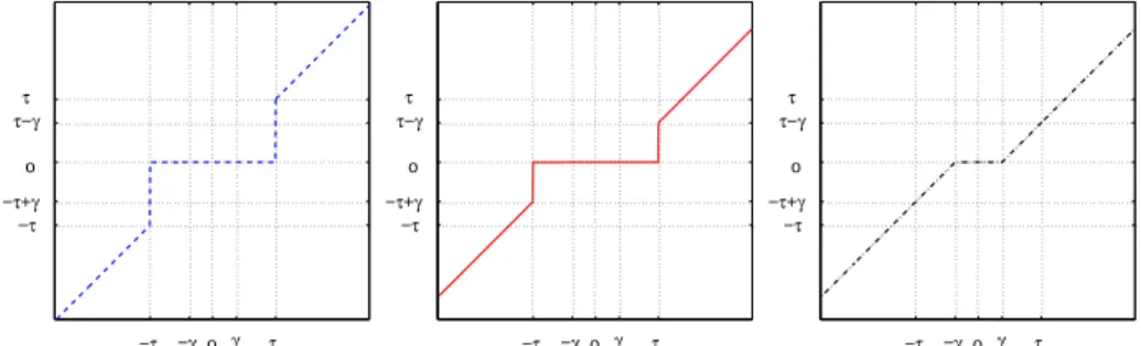
Whenp = 1 and tλ= 1, we obtain a compromise between hard and soft-thresholding if τλ > γwλ. To illustrate this,
we graph in Fig.1 the hard-thresholding function with thresholdτ (left), the soft-thresholding function with threshold γ (right) and the function obtained in Eq.(16) (middle) in the caseτ > γ (here w = 1). We give a further illstration of the diagonal case in Fig. 3, section 5.
−τ τ −τ τ −γ γ τ−γ −τ+γ o o −τ τ −τ τ −γ γ τ−γ −τ+γ o o −τ τ −τ τ −γ γ τ−γ −τ+γ o o
Figure 1. Left: hard-thresholding operator Hτ; middle: adaptive thresholding operator; right: soft-thresholding operator Sγ,1.
3.2.3 Stability is an issue
The study on diagonal operators suggests that introducing adaptive projections gives flexibility by defining a new shrinkage operator. In this section, we see that this flexibility comes to a price: the resulting algorithm is not stable in the sense of Theorem 2.3. There is stability in the sense that if the parameter (τ , w,..) are chosen properly as the noise level decreases - i.e. when the observationg gets closer to the true observation T fo- then the solutions converge to a well-defined limit.
However this limit is not necessarilyfo, even ifT is invertible.
In a nutshell, what happens is that stability requires that the thresholds τ= {τλ}λ∈Λ are large enough compared to
||g − Tfo||. This implies that the subspace defined by the indexes λ such that {Tfo}λ= 0 will necessarily be in the kernel
of the adaptive projectionsMg,τ as soon asg is close enough to Tfo. Therefore the information in this subspace will lost.
The result is then that as the observation becomes ideal (i.e. close toTfo) the solution of Algorithm 3.2 will approach the
element of minimal||| · |||w,p–norm in the setMT,fo of elements ofH
ithat have the same image underT as f
oexcept
maybe on the coordinatesλ such that (Tfo)λ= 0.
Note that even isT is one-to-one, this set is not necessarily reduced to fo:
EXAMPLE1. IfT is the identity, f1= (1, 0) ∈ R2, thenMf1 = {(1, x), x ∈ R} on the canonical basis.
In this case however the minimizer of the||| · |||w,p–norm isf1 itself whatever the choices of the parametersγ, τ , w =
{wλ}λ∈Λ,... are. Algorithm 3.2 will therefore provide the desired result. This is not the case in the following example,
whereT is also an invertible operator in R2:
EXAMPLE2. ConsiderT : R2→ R2, the bounded and linear operator defined by:
T : µ f1 f2 ¶ 7→ 14 µ 2 f1+ f2 f1− f2 ¶ and fa= µ a a ¶ for somea 6= 0.
• T has a bounded inverse: T−1: µ f1 f2 ¶ 7→ 43 µ f1+ f2 f1− 2f2 ¶ and|||T ||| =12< 1. • T fa= µ 3a 4 0 ¶ andMfa = {f : (T f )1= (T fa)1} = {f : 2f1+ f2= 3a}.
The element inMfawith minimall
1norm is:f† a = µ 3a 2 0 ¶
, and notfaitself. Thus the minimizers of Eq.(12) do not
converge tofaas the observations converge toT fa. In other words, information on the second coordinate in image plane
has been lost that prevents the algorithm to invertT even with arbitrary accurate data. We now formalize this result. We first defineMT,fo and the setH
i
T,w,p of elements for whichMT,fo has a unique
minimizer of the||| · |||w,p–norm.
DEFINITION 3.3 (MT,fo). Given two Hilbert spacesH
i and Ho, an operatorT : Hi → Ho, an orthonormal basis
{βλ}λ∈ΛofHoand an elementfoofHi. The setMT,fois the subset of elements ofH
ithat verify:
f ∈ MT,fo ⇐⇒ MTfo,0(Tf ) = Tfo ⇐⇒
h
{Tfo}λ6= 0 ⇒ {Tf }λ= {Tfo}λ
i
DEFINITION3.4 (HiT,w,p). Given a Hilbert spaceHi,Hi
T,w,pis the subset of elements ofHithat verify:fois inHiT,w,p
if and only if the setMT,fo = {f : MTfo,0Tf = Tfo} has a unique element of minimum |||.|||w,p-norm.
Whenp > 1, then Hi
T,w,p = Hi, regardless ofT . This is not true if p = 1, even if ker T = {0}. It turns out that
Algorithm 3.2 is regularizing for elementsf in Hi
T,w,p, and that the minimizer obtained in the limitkTfo− gkHogoes to
zero is exactly the minimizer of the|||.|||w,p-norm inMT,fo. This is the object of the following theorem:
THEOREM 3.5. Assume thatT is a bounded operator from HitoHowith|||T ||| < 1, that γ > 0, p ∈ [1, 2] and that the
entries in the sequence w= {wλ}λ∈Λare bounded below uniformly by a strictly positive numberc.
For anyg ∈ Hoand anyγ > 0 and any nonnegative sequence τ = {τ
λ}λ∈Λ, definefγ,w,p,τ ;g⋆ to be a minimizer of
Jγ,w,p,τ(f ) with observation g. If γ = γ(²) and τ = τ (²) satisfy:
1. lim ²→0γ(²) = 0 and ²→0lim ²2 γ(²) = 0 2. ∀λ ∈ Λ, lim ²→0τλ(²) = 0 and ∃ δ > 0, s.t: [ ² < δ ⇒ ∀λ ∈ Λ, τλ(²) > ² ]
then we have, for anyfo∈ HiT,w,p:
lim ²→0 " sup kg−TfokHo≤² kfγ(²),w,p,τ (²); g⋆ − fo†kHi # = 0 , wheref†
o is the unique element of minimum||| |||w,p–norm in the setMT,fo.
The detailed proof of this theorem is given in3, p.18-24 and is not reproduced here. It is based on two ingredients: • The two lemmas provided in Appendix. A. show that condition 2 in Theorem 3.5 is needed to obtain the weak
convergence of the adaptive projection operatorsMg,τ when||g − Tfo|| → 0.
• Using this weak convergence, one can then adapt the proof of Theorem 2.3 provided in2
.
4. ADAPTIVE DISCREPANCY TERMS (II): RELAXED PROJECTIONS
In the previous section, we showed that introducing adaptive projections in the discrepancy term allows to take into account features that are more important in the data but results in a loss of information that may be harmful to the estimation of the object sought. The reason is that the projections used cancel some information. To fix this instability problem still keeping the spirit of the previous method, one can imagine to only dampen the non-feature space defined by the adaptive projections instead of cancelling it. As we see in the next section, the resulting “relaxed projections” still emphasize the same features but without losing any information; therefore the stability as defined in Theorem 2.3 is restored.
4.1 Relaxed Adaptive Projections
The “relaxed projection” Mg,τ,µ with dampening parameterµ and corresponding to the orthogonal adaptive projection
Mg,τ is
Mg,τ,µ= Mg,τ+µ(Id − Mg,τ) (17)
or more formally:
DEFINITION 4.1. Given an orthonormal basis if Ho, β= {β
λ}λ∈Λ, an element g in Ho, a sequence of nonnegative
thresholdsτ= {τλ}λ∈Λand a scalarµ > 0, Mg,τ,µis the map fromHointo itself defined by:
∀h ∈ Ho, Mg,τ,µ(h) = X λ s.t. |gλ|>τλ hλβλ+ µ X λ s.t. |gλ|≤τλ hλβλ
This operator is introduced in the discrepancy term so that we now seek to minimize the functional Jγ,w,p,τ,µ(f ) =°°Mg,τ,µ(T f − g)°°2
Ho+ γ|||f |||w,p, (18)
via the following iterative algorithm:
ALGORITHM4.2. ½
f0 arbitrary
fn = S
γw,p¡fn−1+ T∗Mg,τ,µ2(g − T fn−1)¢, n ≥ 1
Note that in this case, one needs to square the relaxed projection operator in the iterative algorithm. This is because unlike Mg,τ, Mg,τ,µis not a self-adjoint projection. This equation can be easily checked by replacingT by Mg,τ,µT
andg by Mg,τ,µg in the original functional Jγ,w,p of Eq.(7) and in Algorithm 2.1. In practice, we use the fact that
Mg,τ,µ2= Mg,τ,µ2; so the operator is still easy to compute.
The previous change of variable used in Theorem 2.2 also proves the strong convergence of Algorithm 4.2 to a minimizer of Eq. (18) (under the same conditions as in Theorem 2.2).
4.2 Stability is recovered
The introduction of the dampening factor ensures that all the information in the data will be taken into account and we recover the stability in the usual sense: if the data become ideal (g → Tfo) and the parametersγ, τ = {τλ}λ∈Λandµ are
chosen accordingly, then the solution converges tofowhenfois the unique antecedent ofTfo.
The conditions on the parameters are given in the following theorem:
THEOREM4.3. Assume thatT is a bounded operator from HitoHowith|||T ||| < 1 and that the entries in the sequence
w= {wλ}λ∈Λare bounded below uniformly by a strictly positive numberc.
For anyg ∈ Ho and anyγ > 0, 0 < µ ≤ 1 and nonnegative sequence τ = {τ
λ}λ∈Λ, definefγ,w,p,τ,µ; g⋆ to be a
minimizer of Jγ,w,p,τ,µ(f ) with observation g. If γ = γ(²), τ = τ (²) and µ = µ(²) satisfy:
1. lim ²→0γ(²) = 0 and ²→0lim ²2 γ(²) = 0 2. ∀λ ∈ Λ, lim ²→0τλ(²) = 0 and ∀λ ∈ Λ, ∃ δ(λ) > 0, s.t: [ ² < δ(λ) ⇒ τλ(²) > ² ] 3. lim ²→0µ(²) = µo, with0 < µo≤ 1
then for anyfosuch that there is a unique minimizer of the||| |||w,p–norm in the setSfo= {f : Tf = Tfo}:
lim ²→0 " sup kg−TfokHo≤² kfγ(²),w,p,τ (²),µ(²); g⋆ − fo†kHi # = 0 , wheref†
The proof of this theorem is detailed in3, p.28-31 and is similar to that of Theorem 3.5. The weak convergence of the
adaptive operators is ensured by conditions 2 and 3 of Theorem 4.3 and the corresponding lemma is provided in Appendix B.
It is clear that in practice, by choosingµ small, the properties of g enhanced by both Algorithm 3.2 and 4.2 are similar. The second algorithm is however more stable as it is guaranteed to make a correct guess when the data is sufficiently close to the image of an objectf .
5. APPLICATION
5.1 Multispectral Data
In this section we apply the algorithms described previously to the problem of reconstructing maps of astrophysical phe-nomena from multispectral observations. We consider simulated multispectral observations of the Cosmic Microwave Background (CMB) radiation with the observation conditions relative to the Atacama Cosmology Telescope (ACT). In this case, we observe the same portion of sky at different wavelengthsνl. The observations are blurred mixtures of the physical
phenomena we seekf1,..,fM that can be modeled by:
∀l = 1..L, g(νl) = gl= bl∗ M
X
m=1
am,lfm+ nl. (19)
The blurring bl changes with the wavelength νl and is Gaussian. The mixture coefficientsam,l are called frequency
dependencies and give the contribution of phenomenam to observation l. The noise terms nlhave a known varianceσl
that also depend on the wavelengthνl. Note that here, the operatorTm,lfrom Eq.(2) is a mixture followed by a convolution
Tm,l(·) = bl∗PMm=1am,l(·)m. For ACT, the observation wavelength are low:ν =145, 217 or 265GHz. (Details about
the noise and blur level can be found in3, p.88.) Here, we seek to reconstruct two components:
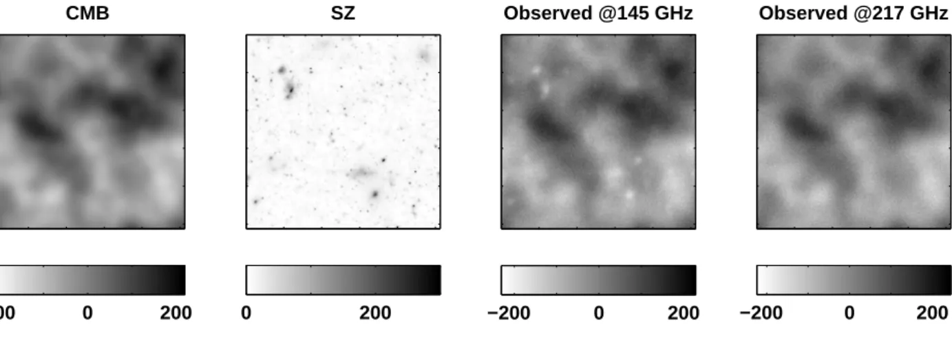
• the CMB (= f1): this is an electromagnetic radiation that fills the whole of the Universe (see Figure 2, left panel).
Its existence and properties are considered one of the major confirmations of the Big Bang theory.
• the galaxy clusters, noted SZ (= f2): the clusters can be seen through their Sunyaev-Zeldovich effect (SZ effect in
short) which is due to high energy electrons in the galaxy clusters that interact with Cosmic Microwave Background photons.
In fact, we focus on the detection and estimation of the galaxy clusters in observations such as can be done with ACT. A complete model of the observations would have to include other astrophysical phenomena such as infrared point sources or our Galaxy dust. We will not consider them here, since their contribution at low wavelengths, such as the ones considered here, are negligible.
Figure 2 illustrates the simulated data we use. The two left panels show the astrophysical map we seek to reconstruct from the observations shown on the two right panels. (The units of the maps is the micro-Kelvin).
General parameters of the functional algorithms
In this multispectral case, the reconstruction methods proposed earlier have one regularization term for each component and one regularization term per observation (see Eq.(3)).
As can be seen from the observations, the contribution of the galaxy clusters (SZ) is negligible compared to this of the CMB. We rely on the fact that these maps have very different spatial properties to disentangle them. These properties are reflected by the regularization terms. The CMB component is regularized by a weightedl2-norm in Fourier space,
the weights being proportional to its spectral power. The SZ component is regularized by anl1-norm on its wavelets
coefficients. The wavelet transform used for regularization is the dual tree complex wavelet transform.4, 5
We compare the results obtained with the classical discrepancy terms of Eq.(3) to these obtained with various adaptive projections, relaxed (Eq.(18)) and not (Eq.(12)). In any case, the adaptive/relaxed projection is done on an orthonormal wavelet transform (Symmlet, 2 vanishing moments) and the threshold parameterτ are set to the noise standard deviation.
SZ 0 200 CMB −200 0 200 Observed @145 GHz −200 0 200 Observed @217 GHz −200 0 200
Figure 2. Multispectral data (units:µK); left to right: CMB map, galaxy clusters map, observation at 145GHz, observation at 217GHz
5.2 Denoising galaxy cluster maps
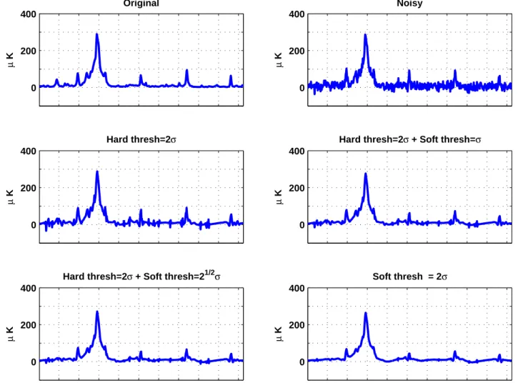
To illustrate the effect of introducing adaptive projections, we took a one-dimensional slice of the galaxy cluster map in Fig. 2 and added noise to it (top panels of Fig. 3) with a standard deviation ofσ.
We show in the four bottom panels of this figure the results of the denoising using • hard-thresholding (Fig. 3, middle left panel) with threshold τ = σ;
• soft-thresholding (Fig. 3, bottom right panel) with threshold γ = σ; This is obtained with the initial iterative algo-rithm (Algo. 2.1).
• the adaptive thresholding (Fig. 3, middle right and bottom left panels) seen in subsection 3.2.2. This is obtained with the adaptive algorithm (Algo. 3.2) Note that there is no stability issue in this example.
One can see that increasing the introduction of the soft-thresholding on top of the hard-thresholding smoothes the solution. The pure soft-thresholding however suffers from that fact that it dampens peaks compared to the pure hard-thresholding. In the case of galaxy clusters, these peak of intensity correspond to the central part of the cluster and indicate its age. Therefore, the dampening obtained by soft-thresholding is detrimental. On the other hand, the lack of smoothness of the hard-thresholded solution will induces false positive in the detection of clusters. The introduction of the adaptive thresh-olding via the use of projections in the discrepancy term allows to tune both effects. It gives an interesting compromise keeping a bit of the advantages of the pure hard or soft-thresholded solutions (see Fig. 3, middle right and bottom left panels).
5.3 Reconstruction of CMB and galaxy clusters maps from multispectral observations
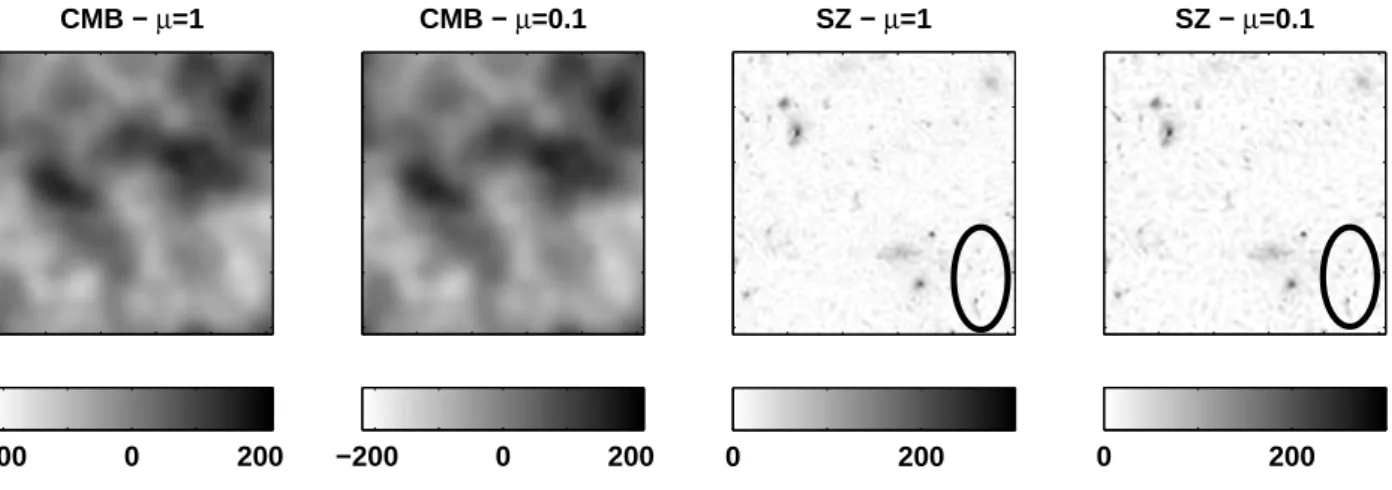
The simultaneous reconstuction of both the CMB and galaxy cluster maps from the multispectral observations as seen in subsection 5.1 has been performed with the different iterative algorithms proposed in section 2, 3 and 4. All parameters were described in 5.1 except for the relaxed projection dampening parameterµ (see Eq.(17)) which is fixed here to µ = 0.1 when using Algorithm 4.2.
Fig. 4 displays the results obtained for
• the initial algorithm (Algo. 2.1) with classical l2discrepancy terms. The results are labelled “µ = 1”.
• the relaxed projection algorithm (Algo. 4.2) with stable adaptive discrepancy terms. The results are labelled “µ = 0.1”.
0 200 400 µ K Original 0 200 400 µ K Noisy 0 200 400 µ K Hard thresh=2σ 0 200 400 µ K
Hard thresh=2σ + Soft thresh=σ
0 200 400
µ
K
Hard thresh=2σ + Soft thresh=21/2σ
0 200 400 µ K Soft thresh = 2σ
Figure 3. Denoising galaxy clusters map. Top left: 1D profile of a cluster map. Top right: noisy 1D profile of a cluster map (noise variance σ2). Middle left: noisy data hard-thresholded (τ = 2σ). Middle right: noisy data soft/hard-thresholded (τ = 2σ, γ = σ). Bottom left: noisy data soft/hard-thresholded (τ = 2σ, γ =√2σ). Bottom right: noisy data soft-thresholded (γ = 2σ).
The observed maps and the CMB and galaxy clusters maps that we seek to recover are in shwon on the left panels of Fig. 2. The reconstructed CMB maps are in the two left panels of Fig. 4. The reconstructed galaxy maps are in the two right panels of Fig. 4.
The following analysis is illustrated by the results shown in 4 but is valid in a more general study with 24 similar simulations.
5.3.1 Analysis of CMB reconstruction
All the reconstructed CMB maps are accurate to the microKelvin precision. The Root Mean Square Error of the different reconstructions to the original (true) CMB map is not affected by the introduction of the adaptive discrepancy term.
The precision obtained for this component is highly satisfactory and allows to proceed to further treatment for astro-physical purposes.
5.3.2 Analysis of the galaxy clusters reconstruction
All the reconstructed galaxy cluster maps have a low accuracy (worst case 100 microKelvin). The Root Mean Square Error of the different reconstructions to the original (true) clusters map is not affected by the introduction of the adaptive discrepancy term. Hence as far as global measures are concerned, all the presented algorithms perform in the same manner
CMB − µ=1 −200 0 200 SZ − µ=1 0 200 CMB − µ=0.1 −200 0 200 SZ − µ=0.1 0 200
Figure 4. Reconstructed maps; without projections: first and third images (µ = 1); with adaptive projections: second and fourth images (µ = 0.1); far/middle left: CMB; far/middle right: galaxy clusters
for galaxy clusters. These poor results are expected by the fact that the contribution of the galaxy clusters to the observation is well below the CMB contribution and the noise level.
However, as explained in,3 global measures are not satisfactory to evaluate the quality of a reconstructed cluster map.
Indeed, the goal is to locate the presence of clusters and quantify some of their statisical characteristics like size, intensity or age... Detailed study of the reliability of these quantities has be done for Algorithm 2.13and show that it actually gives
good results in this prospective. Here, we do not reproduce the all study for Algorithm 3.2 and 4.2 but simply compare them to Algorithm 2.1.
As can be inferred from Fig. 4, the results are very similar. The ontroduction of adaptive discrepancy terms yield a slight improvement in the estimation of the central intensity of a cluster (see the three clusters in the upper part of the circle in Fig. 4). This improvement is not statistically significant however it illustrates how adaptive discrepancy terms provide a novel way of tuning the algorithm to the data.
APPENDIX A. ELEMENTS OF THE PROOF OF THE STABILITY OF (I)
To prove Theorem 3.5, we need to examine the behavior of the projectionsMg(²),τ (²)as² goes to zero. This is done in the
next two lemmas. The first lemma (Lemma A.1) gives necessary and sufficient conditions on the sequence τ= {τλ}λ∈Λto
that these projections converge in a weak sense as² goes to zero. We will be interested in the case where the weak limit operator isMTfo,0. The second lemma (Lemma A.1) refines these conditions, so that in addition, the sequenceMg(²),τ (²)
converges strongly toMTfo,0on the set:T (Mf0).
LEMMA A.1. Forf ∈ Hi, let{g(², f )}
²>0be an arbitrary family of elements inHothat satisfykg(², f ) − Tf kHo < ²,
∀² > 0.
1. ∀h ∈ Ho, M
g(²,f ),τ (²)h converges weakly as ² goes to 0 if and only if ∀λ : ∃ δ(λ) such that either (a) or (b)
holds, with
(a) ∀² ∈ (0, δ(λ)), ¯¯[g(², f)]λ
¯ ¯ > τλ,
(b) ∀² ∈ (0, δ(λ)), ¯¯[g(², f)]λ¯¯ ≤ τλ.
2. Mg(²,f ),τ (²)converges weakly, independently of the choice off and of the family g(², f ), as ² goes to 0 if and only
if ∀λ : both (a) and (b) hold, with
(a) ∃ δ(λ) such that ∀² ∈ (0, δ(λ)), τλ(²) > ²
(b) lim
In that case, the weak-limit operator is necessarilyMTf,0.
3. When conditions 2.(a) and 2.(b) above hold, ifh(²) converges weakly to h, then Mg(²,f ),τ (²)h(²) converges weakly
toMTf,0h as ² goes to 0.
Proof. [Proof of Lemma A.1] Let us examine the behavior of Mg(²,f ),τ (²) coordinate by coordinate. Since
£
Mg(²,f ),τ (²)h¤λequals eitherhλ or0, depending on whether or not
¯
¯[g(², f)]λ
¯
¯ > τλ(²), it follows that Mg(²,f ),τ (²)(h)
will converge weakly as² goes to 0 if and only if for all coordinates λ, one of the following holds: Either there exists someδ(λ) > 0 such that¯¯[g(², f)]λ
¯
¯ > τλ(²) for ² < δ(λ). In this case,£Mg(²,f ),τ (²)h¤λ = hλ for
² < δ(λ).
Or there exists someδ(λ) > 0 such that¯¯[g(², f)]λ
¯
¯ ≤ τλ(²) for ² < δ(λ). In this case,
£
Mg(²,f ),τ (²)h
¤
λ= 0 for ² < δ(λ).
This proves the first assertion.
Let us now consider how uniform this behavior is in the choice of the family g(², f ). Since ¯¯[g(², f) − Tf]λ
¯ ¯ ≤ kg(², f ) − Tf kHo ≤ ², the set of values that can be assumed by |g(², f )λ| is exactly £ Tf − ², Tf + ²¤ (takeg =
Tf + rβλ, r ∈ [−², ²] to reach all the values in this set). Therefore, for a fixed f , the weak convergence of the
op-eratorsMg(²,f ),τ (²), regardless of which sequenceg(², f ) is chosen, is equivalent to putting constraints on the sequence
{τ (²)λ}λ∈Λthat depend of the coordinates(Tf )λ. These constraints depends on whether(Tf )λ6= 0 or (Tf )λ= 0:
• If Tfλ6= 0 then©|g(², f )λ|ª=£|Tfλ|−², |Tfλ|+²¤. Therefore, one needs either:£² < δ(λ) ⇒ τλ(²) > |Tfλ|+²¤
or£² < δ(λ) ⇒ τλ(²) ≤ |Tfλ| − ²¤. In the first case,βλwill always be in the kernel ofMg(²,f ),τ (²)once² < δ(λ).
In the second caseβλwill always in the range ofMg(²,f ),τ (²)once² < δ(λ).
• If Tfλ = 0 then {|g(², f )λ|} = [0, ²]. Therefore one needs [² < δ(λ) ⇒ τλ(²) > ²]. In this case, βλwill always be
in the kernel ofMg(²,f ),τ (²)once² < δ(λ).
Note that we do not know beforehand the value ofTf . To be useful, we must derive requirements on the parameters τλ(²)
that do not depend onf . The minimum requirements on τ (²) ensuring the operators Mg(²,f ),τ (²)converge weakly as²
goes to0 are:
• ∀λ, lim²→0τλ(²) = 0: this ensures that if Tfλ6= 0, we will have τλ(²) < |Tfλ| − ² for sufficiently small ².
• ∀λ, ∃δ(λ) such that ² < δ(λ) ⇒ τλ(²) < ²: this ensures that if Tfλ = 0, we will have τλ(²) < |Tfλ| + ² = ² for
sufficiently small².
If these conditions are satisfied, theMg(²,f ),τ (²)converge weakly as² goes to 0 and one can determine the weak limit:
• for λ s.t. Tfλ6= 0: lim²→0τλ(²) = 0 hence there exists δ(λ, f ) such that ² < δ(λ, f ) implies τλ(²) < |Tfλ| − ². It
follows that:|g(², f )λ| > τλ(²) so that Mg(²,f ),τ (²)(βλ) = βλfor anyg(², f ) and any ² < δ(λ, f )
• for λ s.t. Tfλ = 0: ² < δ(λ) implies τλ(²) > ². It follows that if ² < δ(λ), then |g(², f )λ| > τλ(²) so that
Mg(²,f ),τ (²)(βλ) = 0 for any g(², f ) and any ² < δ(λ) .
This proves that the weak limit ofMg(²,f ),τ (²)for any fixedf is MTf,0and finishes the proof of the second part of Lemma
A.1.
Finally, assumingh(²) converges weakly to h, we have ∀λ: ¯ ¯ ¯£Mg(²,f ),τ (²)h(²) − MTf,0h ¤ λ ¯ ¯ ¯ (20) = ¯¯¯£Mg(²,f ),τ (²)(h(²) − h) + (Mg(²,f ),τ (²)− MTf,0)h¤λ ¯ ¯ ¯ (21) = ¯¯¯£Mg(²,f ),τ (²)(h(²) − h) ¤ λ ¯ ¯ ¯ + ¯ ¯ ¯£Mg(²,f ),τ (²)h − MTf,0h¤λ ¯ ¯ ¯ (22)
The second term vanishes as² goes to 0 because Mg(²,f ),τ (²)converges weakly toMTf,0 when the conditions 2.(a) and
• either there exists a δ(λ) such that Mg(²,f ),τ (²)(βλ) = 0 for any ² < δ(λ) . In that case, ¯ ¯ ¯£Mg(²,f ),τ (²)(h(²) − h) ¤ λ ¯ ¯ ¯ = 0, for ² < δ(λ).
• or there exists a δ(λ) such that Mg(²,f ),τ (²)(βλ) = βλfor any² < δ(λ) .
In that case, ¯ ¯ ¯£Mg(²,f ),τ (²)(h(²) − h) ¤ λ ¯ ¯ ¯ = ¯ ¯
¯£h(²) − h¤λ¯¯¯, for ² < δ(λ); and the weak convergence of h(²) to h allows to conclude that
¯ ¯ ¯£Mg(²,f ),τ (²)(h(²) − h)¤λ ¯ ¯ ¯ → 0
This proves thatMg(²,f ),τ (²)h(²) converges weakly to MTf,0h and finishes the proof of Lemma A.1.
We shall now see how to ensure strong convergence of theMg(²,f ),τ (²)(h) when h is in Mf.
LEMMA A.2. If there exists a value ofδ independent of λ such that ∀² < δ and ∀λ, τλ(²) > ², then the two following
properties hold:
1. For any choice off and of the family g(², f ):
∀² < δ, Mg(²,f ),τ (²)= MTf,0Mg(²,f ),τ (²)= Mg(²,f ),τ (²)MTf,0=
X
λs.t.Tfλ6=0
and|gλ|≥τλ
h ., βλi βλ.
2. In particular, for any choice off ∈ Hi
T,w,pand of the familyg(², f ), (i.e. whenever Mfhas a unique minimizerf†
of the|||.|||w,p-norm):
∀² < δ, Mg(²,f ),τ (²)(Tf†) = Mg(²,f ),τ (²)(Tf ).
Proof. [Proof of Lemma A.2:] The first part of Lemma A.2 results from properties of orthogonal projections. IfP1and
P2are two orthogonal projections, then:
P1P2 = P2P1
ker(P2) ⊂ ker(P1) ⇔ P1P2= P1.
Hence, we already provedMg(²,f ),τ (²)MTf,0= MTf,0Mg(²,f ),τ (²)and
Mg(²,f ),τ (²)MTf,0 = Mg(²,f ),τ (²)⇔
£
(Tf )λ= 0 ⇒ |g(²,f )λ| ≤ τλ(²)
¤ . Whenf and ² are fixed, the right hand side holds for any g(², f ) if and only if£(Tf )λ= 0 ⇒ ² < τλ(²)
¤
which proves the first part of Lemma A.2.
Forf in Hi
T,w,p,f†is well defined and verifiesMTf,0Tf† = Tf . Applying Mg(²,τ (²))to this equality and using the
previous result finishes the proof of Lemma A.2.
APPENDIX B. ELEMENTS OF THE PROOF OF THE STABILITY OF (II)
LEMMA B.1. Suppose thatτ = τ (²) and µ = µ(²) verify conditions 2 and 3 of Theorem 4.3. Then the two following
properties hold:
1. For anyh in Ho,M2
g(²,f ),τ (²),µ(²)h converges weakly to M 2
Tf,0,µoh as ² goes to 0.
2. Ifh(²) converges weakly to h as ² goes to 0, then M2
g(²,f ),τ (²),µ(²)h(²) converges weakly to M 2
Tf,0,µoh as ² goes to
0.
Proof. [ Proof of Lemma B.1:] In the proof of Lemma A.1, we have seen that under conditions imposed onτ (²) (conditions 3 and 4 of Theorem 4.3), the following happens:
• for λ s.t. Tfλ6= 0: lim²→0τλ(²) = 0 hence there exists δ(λ, f ) such that ² < δ(λ, f ) implies τλ(²) < |Tfλ| − ². It
• for λ s.t. Tfλ= 0: ² < δ(λ) implies τλ(²) > ². It follows that if ² < δ(λ), then |g(², f )λ| > τλ(²).
So that in the first case: M2
g(²,f ),τ (²),µ(²)(βλ) = βλ for any g(², f ) and any ² < δ(λ, f ); and in the second case:
M2
g(²,f ),τ (²),µ(²)(βλ) = µ(²) 2β
λ for anyg(², f ) and any ² < δ(λ). Since µ(²) converges to some µo by assumption
(condition 5 of Theorem 4.3), it follows thatMg(²,f ),τ (²),µ(²)2 h converges to MTf2o,0,µoh as (²) goes to 0. This proves the
first part of Lemma B.1.
To prove the second part of Lemma B.1, we use again the splitting trick we used in A.1.(3): ¯ ¯ ¯£Mg(²,f ),τ (²),µ(²)2 h(²) − M2Tf,0,µoh ¤ λ ¯ ¯ ¯ (23) = ¯¯¯£Mg(²,f ),τ (²),µ(²)2 (h(²) − h) + (Mg(²,f ),τ (²),µ(²)2 − M 2 Tf,0,µo)h ¤ λ ¯ ¯ ¯ (24) = ¯¯¯£M2 g(²,f ),τ (²),µ(²)(h(²) − h) ¤ λ ¯ ¯ ¯ + ¯ ¯ ¯£(M2 g(²,f ),τ (²),µ(²)− M 2 Tf,0,µo)h ¤ λ ¯ ¯ ¯ (25)
And the same argument as we used in Lemma A.1.(3) allows to conclude.
ACKNOWLEDGMENTS
Most of this work was done in Princeton University, during the Ph.D of S.A supported by the BWF training program. The author would like to thank her collaborator Elena Pierpaoli for providing the astrophysical problem and data at the basis of this work, and her Ph.D. advisor Ingrid Daubechies.
REFERENCES
1. J.-L. Starck, F. Murtagh, and A. Bijaoui, “Multiresolution support applied to image filtering and restoration,” Graphical
Models and Image Processing 57, pp. 20–431, 1995.
2. I. Daubechies, M. Defrise, and C. De Mol, “An iterative thresholding algorithm for linear inverse problems with a sparsity constraint,” Comm. Pure Appl. Math. 57, pp. 1413–1541, 2004.
3. S. Anthoine, Different Wavelet-based Approaches for the Separation of Noisy and Blurred Mixtures of Components.
Application to Astrophysical Data. Ph.d. dissertation, Princeton University, 2005.
4. N. G. Kingsbury, “Complex wavelets for shift invariant analysis and filtering of signals,” Journal of Applied and
Computational Harmonic Analysis 10(3), pp. 234–253, 2001.
5. I. W. Selesnick, “The design of approximate hilbert transform pairs of wavelet bases,” IEEE Transactions on Signal