HAL Id: hal-00859363
https://hal.archives-ouvertes.fr/hal-00859363
Submitted on 11 Sep 2013
HAL is a multi-disciplinary open access
archive for the deposit and dissemination of
sci-entific research documents, whether they are
pub-lished or not. The documents may come from
teaching and research institutions in France or
abroad, or from public or private research centers.
L’archive ouverte pluridisciplinaire HAL, est
destinée au dépôt et à la diffusion de documents
scientifiques de niveau recherche, publiés ou non,
émanant des établissements d’enseignement et de
recherche français ou étrangers, des laboratoires
publics ou privés.
search
Djamal Belazzougui, Adeline Pierrot, Mathieu Raffinot, Stéphane Vialette
To cite this version:
Djamal Belazzougui, Adeline Pierrot, Mathieu Raffinot, Stéphane Vialette. Single and multiple
con-secutive permutation motif search. ISAAC 2013, Dec 2013, Hong-Kong, Hong Kong SAR China.
pp.66-77, �10.1007/978-3-642-45030-3_7�. �hal-00859363�
motif search
Djamal Belazzougui?, Adeline Pierrot??,
Mathieu Raffinot⇤⇤, and St´ephane Vialette? ? ?
Abstract:Let t be a permutation (that shall play the role of the text) on [n] and a pattern p be a sequence of m distinct integer(s) of [n], m ≤ n. The pattern p occurs in t in position i if and only if p1. . . pmis order-isomorphic to ti. . . ti+m−1, that is, for
all 1 ≤ k < ` ≤ m, pk > p` if and only if ti+k−1> ti+`−1. Searching for a pattern p
in a text t consists in identifying all occurrences of p in t. We first present a forward automaton which allows us to search for p in t in O(m2log log m + n) time. We then
introduce a Morris-Pratt automaton representation of the forward automaton which allows us to reduce this complexity to O(m log log m + n) at the price of an additional amortized constant term by integer of the text. Both automata occupy O(m) space. We then extend the problem to search for a set of patterns and exhibit a specific Aho-Corasick like algorithm. Next we present a sub-linear average case search algorithm running in O⇣m log m
log log m+ n log m m log log m
⌘
time, that we eventually prove to be optimal on average.
1
Introduction
Two sequences are order-isomorphic if the permutations required to sort them are the same. A sequence p is said to be a pattern (or occurs) within a sequence t if t has a subsequence that is order-isomorphic to p. Pattern involvement per-mutations and sequences has now become a very active area of research [10]. However, only few results on the complexity of finding patterns in permutations and sequences are known. It appears to be a difficult problem to decide of two given permutations ⇡ and σ whether σ occurs in ⇡, and in this generality the problem is NP-complete [7]. For σ2 Smand ⇡2 Sn, the O(nm) time brute-force
algorithm was improved to O(n0.47m+o(m)) time in [2]. There are several ways
in which this notion of permutation patterns may be generalized, and we focus here on consecutive patterns (i.e. the match is required to consist of contiguous elements) [10]. A sequence p is said to be a consecutive pattern or consecutively occurs within a sequence t if t has a substring that is order-isomorphic to p. Searching for a pattern p in a text t consists in identifying all occurrences of p in t. Recently, using a modification of the classical Knuth-Morris-Pratt string matching algorithm, a O(n + m log m) time algorithm has been proposed for checking if a given sequence t of length n contains a substring which is order-isomorphic to a given pattern p of length m [11]. The time complexity reduces to O(n + m) time under the assumption that the symbols of the pattern can be sorted in O(m) time.
The set of all integers from 1 to n is written [n]. Let t be a permutation of length n and p be a sequence of m n distinct integers in [n]. First we present
?
Department of Computer Science, FI-00014 University of Helsinki, Finland
??
LIAFA, Univ. Paris Diderot - Paris 7, 75205 Paris Cedex 13, France
? ? ?
a forward automaton which allows us to search for p in t in O(m2log log m + n)
time. Next, we introduce a Morris-Pratt automaton representation [9] of the for-ward automaton which allows us to reduce this complexity to O(m log log m + n) at the price of an additional amortized constant term by integer of the text. Both automata occupy O(m) space. We then extend the problem to search for a set of patterns and exhibit a specific Aho-Corasick like algorithm. Finally we present a sub-linear average case search algorithm running in O(n log m/ log log m) time that we eventually prove to be optimal on average. Both lower and upper bounds assume all text permutations to be equiprobable and all integer values in a pat-tern to be distinct.
Let us define some notations. The set of all permutations on [n] is denoted by Sn. Let ⌃n = [n]. Abusing notations, we consider in this paper permutations
of Sn as strings without symbol repetition, and we denote by ⌃n⇤ the set of
all strings without symbol repetition (including the empty string), where each symbol is an integer in [n]. A prefix (resp. suffix, factor) u of p is a string such that p = uw, w 2 ⌃⇤
n. (resp. p = wu, w 2 ⌃⇤n, p = wuz, w, z2 ⌃n⇤. We also denote
|w| the number of integer(s) in a string w, w 2 ⌃⇤
n. We eventually denote prthe
reverse of p, that is, the string formed by the symbols of p read in the reverse order. We denote by p⌘ the set of words of ⌃⇤
n which are order-isomorphic to p.
The following property is useful for designing automaton transitions. Property 1. Let p = p1. . . pm2 ⌃n⇤and w = w1. . . w`2 ⌃n⇤, ` < m, such that w
is order-isomorphic to p1. . . p`, and let ↵2 ⌃. Testing if w↵ is order-isomorphic
to p1. . . p`p`+1can be performed in constant time storing only a pair of integers.
Proof. The pair of integers (x1, x2) is determined as follows: x1 ` is the
position of the largest number px1 in p1..p` which is smaller than p`+1, if any.
Otherwise, we fix x1arbitrarily to−1. Let x2 ` be the position of the smallest
integer px2 in p1..p` which is larger than p`+1, if any. Otherwise, we fix x2 to
+1. Now, it suffices to test if wx1< ↵ < wx2 to verify if w↵ is order-isomorphic
to p1. . . p`+1 ut
We define a function rep(p = p1. . . pm, j) which returns a pair of integers
(x1, x2) that represents the pair defined in property 1 for the prefix of length j
of a motif p.
2
Tools
Before proceeding, we first describe some useful data structures we shall use as basic subroutines of our algorithms. The problem called predecessor search problem is defined as follows: given a set S ={x1, x2, . . . xn} ⇢ [u] (u is called the
size of the universe), we support the following query: given an integer y return its predecessor in the set S, namely the only element xi such that xi y xi+1 1.
In addition, in the dynamic case, we also support updates: add or remove an
1 By convention, if all the elements of S are smaller than y, then return −∞ and if
element from the set S. The standard data structures to solve the predecessor search are the balanced binary search trees [1,5]. They use linear space and support queries and updates in worst-case O(log n) time. However, there exists better data structures that take advantage of the structure of the integers to get better query and update time. Specifically, the Van-Emde-Boas tree [14] supports queries and updates in (worst-case) time O(log log u) using O(u) space. Using randomization, the y-fast trie achieves linear space with queries supported in time O(log log u) and updates supported in randomized O(log log u) time. The problem has received series of improvements which culminated with Andersson and Thorup’s result [4]. They achieve linear space with queries and updates supported in O(min(log log u,qlog log nlog n )) (the update time is still randomized). A special case occurs when space n is available and the set of keys S is known to be smaller than logcn for some constant c. In this case all operations are supported in worst-case constant time using the atomic-heap [15].
3
Forward search automaton
The problem we consider is to search for a motif p in a permutation t without preprocessing the text itself. By analogy to the simpler case of the direct search of a word p in text t, we build an automaton that recognizes (⌃⇤
n) ˙p⌘. We then
prove its size to be linear in the length of the pattern.
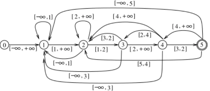
We formally define our forward search automatonFD(p) built on p = p1. . . pm
as follows: (i) m + 1 states corresponding to each prefix (including the empty prefix) of p, state 0 is initial, state m is terminal; (ii) m forward transitions from state j to j + 1 labeled by rep(p, j + 1); (iii) bt backward transitions δ(x, [i, j]), where x numbers a state, 0 x m, i 2 1, . . . , x [ −1, j 2 1, . . . , x [ +1, defined the following way: δ(x, [i, j]) = q if and only if for all pi< ↵ < pj (resp.
k = ↵ < pj if i = −1, pi < ↵ if j = +1), the longest prefix of p that is
order-isomorphic to a suffix of p1. . . px↵ is p1. . . pq. We also impose some
con-straints on outgoing transitions. Let x be a given state corresponding to the prefix p1. . . px. +∞] ∞ − [ , [1,2 ] [2,+∞] +∞] , 2 [ , 2 [ 4 ] ∞ − [ ,1] ∞ − [ ,1] ∞ − [ , 3] ∞ − [ , 3] , 5 [ 4 ] +∞] , 4 [ +∞] , 4 [ ∞ − [ , 5] , 3 [ 2 ] , 3 [ 2 ] 0 1 2 3 4 5 , 1 [ +∞]
Fig. 1. Forward automaton built on p = 4 12 6 16 10. State 0 is initial and state 5 is terminal.
Let us sort all pi, 1
i x and consider the resulting order pi0 =
−1 < pi1 < . . . <
pik < +1 = pik+1.
We build one outgoing transition for each inter-val [pij, pij+1], excepted if
pij+1 = pij + 1. Also we
merge transitions from the same state to the same state that are la-beled by consecutive in-tervals.
It is obvious that the resulting automaton recognizes a given pattern in a permutation by reading one by one each integer and choose the appropriate transition. Figure 1 shows such an automaton. The main result on the structure of the forward automaton is the following.
Lemma 1. The number of transitions of the forward automaton built on p1. . . pm
is linear in m.
Lemma 1 combined with the fact that the outgoing transitions from each state q are sorted accordingly to the closest proximity to q of their arrival state leads to the following lemma.
Lemma 2. Searching for a consecutive motif p = p1. . . pm in a permutation
t = t1. . . tn using a forward automaton built on p takes O(n) time.
We can build the forward automation in O(m2log log m) time. However, we
defer the proof of this construction for the following reason. This O(m2log log m)
complexity might be too large for long patterns. Nevertheless, we show below that we can compute in a first step a type of Morris-Pratt coding of this au-tomaton which can either (a) be directly used for the search for the pattern in the text and will preserve the linear time complexity at the cost of an amortized constant term by text symbol, or (b) be developed to build the whole forward automaton structure.
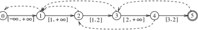
Therefore we present and build a new automatonMP that is a Morris-Pratt representation of the forward automaton. The idea is to avoid building all back-ward transitions by only considering a special backback-ward single transition from each state x, x > 0 named failure transition. We formally define our automaton MP (p) built on p = p1. . . pmthe following way: (i) m + 1 states corresponding
to each prefix (including the empty prefix) of p, state 0 is initial, state m is terminal; (ii) m forward transitions from state j to j + 1 labeled by rep(p, j + 1); (iii) m failure transitions (non labeled) defined by: a failure transition connects a state j > 0 to a state k < j if and only if p1. . . pk is the largest order-isomorphic
border of p1. . . pj. Figure 2 shows such an MP automaton.
+∞] ∞ − [ , [1,2 ] [2,+∞] [3,2 ] 0 1 2 3 4 5 , 1 [ +∞]
Fig. 2. MP automaton built on p = (4, 12, 6, 16, 10). State 0 is initial and state 5 is terminal. Backward transitions are failure transitions.
Reading a text t through the MP representation of the forward automaton is performed the following way. Let us assume we reached state x < m and we read a symbol ti at position i of the text. Let [k, `] = rep(p, x + 1). If ti 2
[ti−m+k, ti−m+l] we follow the forward transition and the new current state is x + 1. Otherwise, we fail reading ti from x and we retry from state q = fail(x)
and so-on until (a) either q is undefined, in which case we start again from state 0, either (b) a forward transition from q to q + 1 works, in which case the next current state is q + 1.
Lemma 3. Searching for a pattern p in a text t1. . . tm using the Morris-Pratt
representation of the forward automaton built on p is O(n) time.
In order to prove lemma 3 we need to focus on the classical notion of border that we extend to our framework.
Definition 1. Let p 2 ⌃⇤
n. A border of p is a word w⌃n⇤,|w| < |p| that is
order-isomorphic to a suffix of p but also order-isomorphic to a prefix of p. The construction of the forward automation relies of the maximal border of each prefix that is followed by an appropriate integer in the pattern. The Morris-Pratt approach is based on the following property:
Property 2. A border of a border is a border.
This property allows us to replace the direct transition of the forward algo-rithm by a search along the borders, from the longest to the smallest, to identify the longest one that is followed by the appropriate integer. We prove now that we can build the Morris-Pratt representation of the forward automaton efficiently. Lemma 4. Building an Morris-Pratt representation of the forward automa-ton on a consecutive motif p = p1. . . pm can be performed in (worst-case)
O(m log log m) time.
Lemma 3 and 4 allow us to state the main theorem of this section.
Theorem 1. Searching for a consecutive motif p = p1. . . pm in a permutation
t = t1. . . tn can be done in O(m log log m + n) time.
The Morris-Pratt representation of the forward automaton permits to search directly in the text at the price of larger amortized complexity (considering the constant hidden by the O notation) than that required by searching with the forward automaton directly. If the real time cost of the search phase is an issue, the forward automaton can be built form its Morris-Pratt representation as follows.
Property 3. Building the forward automaton of a consecutive motif p = p1. . . pm
can be performed in O(m2log log m) time.
An interesting point is that the construction of the forward automaton from its Morris-Pratt representation can also be performed in a lazy way, that is, when reading the text. The missing transitions are then built on the fly when needed.
4
Multiple worst case linear motif searching
We can extend the previous problem defined for a single pattern to a set of patterns S. We note by d the number of patterns, by m the total length of the patterns and by r the length of the longest pattern. For this problem we adapt the Aho-Corasick automaton [3] (orAC automaton for short). The AC automaton
is a generalization of theMP automaton to a set of multiple patterns. We note by P the set of prefixes of strings in S. In order to simplify the description we will assume that the set of patterns S is prefix-free. That is, we will assume that no pattern is prefix of another. Extending the algorithm to the case where S is non-prefix free, should not pose any particular issue. The states of theAC automaton are defined in the same way as in the MP automaton. Each state t in the AC automaton corresponds uniquely to a string p2 P . The forward transitions are defined as follows: there exists a forward transition connecting state s to each state corresponding to an element pc 2 P (where c is a single symbol). Thus this definition of the forward transitions matches essentially the definition of the forward transitions in the MP automaton. The failure transitions are defined as follows: a failure transition a state s corresponding a string p to the state s0
corresponding to the longest string q such that q2 P and q 6= p. The matching using the AC automaton is done in the same way as in the MP automaton using the forward and failure transitions.
Our extension of the AC automaton. We could use exactly the same algorithm as the one used previously for our variant of theMP automaton with few differences. We describe our modification to AC automaton to adapt it to the case of consecutive permutation matching. An important observation is that we could have two or more elements of P that are both of the same length and order-isomorphic. Those two elements should have a single corresponding state in theAC automaton. Thus, if two or more elements of P are order-isomorphic then we keep only one of them. For the forward transitions, we can a associate a pair of positions (x1, x2) to each forward transition. Then we can check which
transition is the right one by checking the condition ti−m+x1 < ti < ti−m+x2
for every pair (x1, x2) and take the corresponding transition. The main problem
with this approach is that the time taken would grow to O(d) time to determine which transition to take which can lead to a large complexity if d is very large. Our approach will instead be based on using a binary search tree (or more sophisticated predecessor data structure). With the use of a binary search tree, we can achieve O(log r) time to decide which transition to take. More precisely, each time we read ti we insert the pair (ti, i) into the binary search tree. The
insertion uses the number ti as a key. Now suppose that we only pass through
forward transitions. Then a transition at step i is uniquely determined by: (1) the current state s corresponding to an element p2 P ; (2) the position of the predecessor of ti among ti−|p|. . . ti−1.
To determine the predecessor of ti among ti−|p|. . . ti−1, the binary search
tree should contain precisely the|p| pairs corresponding to ti−|p|]. . . ti−1. If the
predecessor of tiin the binary search tree is a pair (tj, j), we then conclude that
the element p[|p| − j + 1] is the predecessor of ti in p.
In order to maintain the binary search tree we must do the following actions during passing through a failure or a forward transition: (1) whenever we pass through a forward transition at a step i we insert the pair (ti, i); (2) whenever
to a state corresponding to a prefix p2, then we should remove from the binary
tree all the pairs corresponding to the symbols ti−|p1|. . . ti−|p2|.
It should be noted that each removal or insertion of a pair into the binary search tree takes O(log r) time. The upper bound O(log r) comes from the fact that we never insert more than r elements in the binary search tree. Since in overall we are doing O(n) insertions or removals, the amortized time should simplify to O(n log r). Finally if we replace binary search tree with a more ef-ficient predecessor data structure, we will be able to achieve randomized time O(n· t) where t = min(log log n,qlog log rlog r , d) is the time needed to do an op-eration on the predecessor data structure (see section 2 for details). We use the linear space version of the predecessor data structure which guarantees only randomized performance but uses O(r) additional space only. We thus have the following theorem :
Theorem 2. Searching for set of d consecutive motifs of maximal length r and whoseAC automaton has been built and where the longest pattern is of length r can be done in randomized O(nt) time, where t = min(log log n,qlog log rlog r , d).
Preprocessing. We now show that the preprocessing phase can be done in worst-case O(m log log r) time. As before our starting point will be to sort all the patterns and reduce the range of symbols of each pattern of length ` from range [n] to the range [1..`]. This takes worst-case time O(m log log r).
Recall that two or more elements of P of the same length and order-isomorphic should be associated with the same state in the AC automaton. In order to identify the order-isomorphic elements of P , we will carry a first step called nor-malization. It consists in normalizing each pattern. A pattern p is normalized by replacing each symbol pj by the pair rep(p = p1. . . pj−1, j) (consisting in
the positions of the predecessor and successor among symbols p1. . . pj−1). This
can be done for all patterns in total O(m log log r) time. In the next step, we build a trie on the set of normalized patterns. This takes linear time. The trie naturally determines the forward transitions. More precisely any node in the trie will represent a state of the automaton and the the labeled trie transitions will represent follow transitions.
Note that unlike the forward automaton (or theMP automaton) there could be more than one outgoing forward transition from each node. In order to en-code the outgoing transition from each node, we will make use of a hash table that stores all the transitions outgoing from that node. More precisely for each transition labeled by the pair rep(p = p1. . . pj−1, j) and directed to a state q,
the hash table will associate the key p1 associated with the value q. Now that
the next transitions have been successfully built, the final step will be to build the failure transitions and this takes more effort. The construction of the failure transitions can also be done in worst-case O(m log log r) time, but for lack of space we defer the details to the appendix.
Theorem 3. Building the AC automaton for a set of d consecutive motifs of total length m and where the longest motif is of length r can be done in worst-case O(m log log r) time.
5
Single sublinear average-case motif searching
Algorithm forward takes O(n + m log log m) time in the worst case time but also on average. We present now a very simple and efficient average case-algorithm which takes O(log log mm log m + nm log log mlog m ) time.
In order to search for a pattern p in t, we first build a tree T of all isomorphic-order factors of prof length 3.5 log m
log log m. T is built by inserting each such factor one
after the other in a tree and building the corresponding path if it does not already exist. The construction of this tree requires O(log log mm log m) time (details are given below). The search phase is performed through a window of size m that is shifted along the text. For each position of this window, b = 3.5 log mlog log m symbols are read backward from the end of the window in the tree T . Two cases may occurs: (i) either the factor is not recognized as a factor of pr. This means that no occurrence
of p might overlap this factor and we can surely shift the search window after the last symbol of this factor; (ii) either the factor is recognized, in which case we simply check if the motif is present using a naive O(m) algorithm, and we repeat this test for the next O(m/2) symbols. This might require O(m2/2) steps
in the worst case.
Let us analyze the average complexity of our algorithm, in the following model: all text permutations are considered to be equiprobable, all integer values in a pattern are distinct.
We count the average number of symbol comparisons required to shift the search window of m/2 symbols to the right. As there are 2n/m such segments of length m/2 symbols in n, we will simply multiply the resulting complexity by 2n/m to gain the whole average complexity of our algorithm.
There might be O(b!) distinct motifs that could appear in the text while this number is bounded by m− b + 1 in the pattern (one by position). Thus, with a probability bounded by m−b+1b! we will recognize the segment of the text as a factor of p and enter case 2. In which case, moving the search window of m/2 symbols to the right using the naive algorithm will require O(m2/2) worst case time.
In the other case which occurs with probability at least 1−m−b+1
b! , shifting
the search window by m/2 symbols to the right only requires reading b numbers. The average complexity (in terms of number of symbol reading and compar-isons) for shifting by m/2 symbols is thus (upper) bounded by A = O((m2/2)m−b+1
b! +
b(1−m−b+1b! )) and the whole complexity by O((2n/m)A). By expanding and sim-plifying A we get that A = O(b + O(m3/2b!)). Now using the famous Stirling
approximation ln(m!) = m ln m− m + O(ln m), it is not difficult to prove that b! = 2b log b−b log e+O(log b) = ⌦(m3) and thus A = O(b) and the whole average
time complexity (in terms of number of symbol reading and comparisons) turns out to be O(m log log mn log m ).
Implementation details. The tree T can actually be built in O(log log mm log m) time by using appropriate data structures. Recall that the tree T recognizes all the factors of pr of length 3.5 log m
log log m. To implement T , we use the same AC
automaton presented in previous section to build the tree T , but with two differ-ences: we only need forward transitions and the length of any pattern is bounded by log log mlog m . Thus the cost is upper bounded by O(log log mm log m · t), where t is the time needed to do an operation on the predecessor data structure (maximum of the times needed for inserts/deletes and searches) We now turn our attention to the cost of the matching phase. From the previous section, we know that the total complexity in terms of number of symbol reading and comparisons is O(m log log mn log m ). The total cost of the matching phase is dominated by the multi-plication of the total number of text symbols read multiplied by the cost of a transition in the AC automaton which itself is dominated by the time to do an operation on a predecessor data structure. The total cost of the matching phase is thus O(m log log mn log m · t), where t is the time needed to do an operation on the predecessor data structure.
Now the performance of both matching and building phases crucially depend on the used predecessor data structure. If a binary search tree is used then t = O⇣loglog log mlog m ⌘ = O(log log m) and the total matching time becomes O(nt) = O(n log log m), and the total building time becomes O(m log m). However, we can do better if we work in the word-RAM model. Namely, we can use the atomic-heap (see section 2) which would add additional o(m) words of space and support all operations (queries, inserts and deletes) in constant time on sets of size logO(1)m. In our case, we have a set of size O(log log mlog m ) and thus the operations can be supported in constant time. We thus have the following theorem:
Theorem 4. Searching for a consecutive motif p = p1. . . pm in a permutation
t = t1. . . tn can be done in average O(log log mm log m +m log log mn log m ) time.
6
Average optimality
We prove in this section a lower bound on the average complexity of any consec-utive motif matching algorithm. The proof of this bound is inspired by that of Yao [16] which proved an average lower bound for matching a pattern of length m in a text of length n. We prove in our case of interest an average lower bound of ⌦(m log log mn log m ) considering all permutations over [n] to be equiprobable. As this average complexity is reached by the algorithm we designed in the previous section, this bound is tight.
We begin to circumscribe our problem on small segments of length 2m− 1 of the text into which we search for. Precisely, following [16,12], we divide our text inbn/(2m − 1)c contiguous and no-overlapping segments si, 1 bn/(2m − 1)c,
such that si(t) = t(2m−1)(i−1)+1. . . t(2m−1)i. When searching for a pattern in t,
there might be occurrences overlapping two blocks. But as we are interested on a lower bound, the following lemma allows us to focus on all segments.
Lemma 5. A lower bound for finding a pattern p inside all segments si(t) is
also a lower bound to the problem of searching for all occurrences of p in t. We now prove that instead of focusing on all segments si(t), we can focus on
obtaining a lower bound to search p in any single segment and then extend the lover bound on searching for p inside this segment to searching for p inside all segments, and thus, using the previous lemma, to the whole text.
Lemma 6. The average time for searching for p inside all segments si(t) is
bn/(2m−1)c times the average time for searching for p inside any such segment. Let E(t) be the average complexity for searching p in any segments. Using the previous lemma, the whole average complexity isPbn/(2m−1)c
i=1 E(t) =bn/(2m −
1)cE(t) = ⌦(n/m)E(t).
We now prove a lower bound for E(t), which, using the two previous lemma, gives us a lower bound for the whole problem. LetPm(`) the number of
permu-tations of size m that can be discarded using a sliding window of size m over a text of size 2m− 1 and checking only 0 < ` m positions in this window. Lemma 7 (Counting lemma). Let 0 < ` m. Then |Pm(`)| m!%1 − `!1&d
m−1 `2 e.
Let us consider now the whole set Sm of permutations of length m which
contains m! such permutations. Given 1 < l(m) m, this set is the union of two distinct setPm(`) and Sm\ Pm(`), that is the set of motifs discarded by a
certificate of length l (or by l accesses) and the others. For all pattern inPm(`),
the average complexity to be discarded is counted 1. For any other motif in Sm\ Pm(`), the average complexity is at least l + 1.
The average complexity for discarding all patterns in Sm is thus C(m) = |Pm(`)|+(m!−|Pm(`)|)(l+1)
m! . We aim to find l(m) that maximizes this expression
when m grows, which will provide us a lower bound for the whole average com-plexity. Now let us consider a fixed l(m). We need to lower bound C(m). As C(m) decreases whenPm(`) increases, this lower bound is minimal whenPm(`)
is as large as possible. Then, as the counting lemma states that |Pm(`)|
m!%1 − 1 `!
&dm−1`2 e , C(m) is minimal when |P
m(`)| = m!%1 − `!1&d
m−1 `2 e . We
now arbitrarily impose 98/100 |Pm(`)|
m! 99/100. With the left constraint,
C(m)≥ l − 98/100l + 1 = ⌦(l). We want to compute l(m) such that 98/100
|Pm(`)|
m! =%1 −
1 `!
&dm−1`2 e 99/100. Let us impose ⌃m−1
`2 ⌥ ⇥
1
l! 1/10 (ineq.1).
This allows us to approximate our equation using the classical formula (1+x)a=
1 + ax +a(a−1)2! x2+ . . . + a!
n!(a−n)!xn = 1 + ax + γ where a =
⌃m−1
`2 ⌥, x = −1l!
and γ =Pn
i=2 i!(a−i)!a! xi. It is easy to see that inequality (1) implies that γ
con-verges and is dominated by its first term which is bounded a(a−1)2! x2 1/200. We thus deduce that (1 + x)a
2 [1 + ax, 1 + ax + 1/200] which implies that (1 + x)a− 1/200 1 + ax (1 + x)a. From (1 + x)a = |Pm(`)| m! 2 [ 98 100, 99 100], we obtain 10098 − 1 200 1 + ax 99
100. By replacing a and x in 1 + ax we get
: 10098 − 1 200 = 195/200 1 − ⌃m−1 `2 ⌥ ⇥ 1 l! 99/100. We prove in appendix
that l = log log mb log m with b = 1 + o(1) verify these two inequalities and inequality (1). Thus ⌦(m log log mn log m ) is a lower bound of the whole average complexity for searching for a consecutive motif in a permutation.
References
1. M. AdelsonVelskii and E.M. Landis. An algorithm for the organization of infor-mation. Defense Technical Information Center, 1963.
2. S. Ahal and Y. Rabinovich. On Complexity of the Subpattern Problem. SJDM, 22(2):629–649, 2008.
3. A. V. Aho and M. J. Corasick. Efficient string matching: An aid to bibliographic search. Commun. ACM, 18(6):333–340, 1975.
4. A. Andersson and M. Thorup. Dynamic ordered sets with exponential search trees. J. ACM, 54(3):13, 2007.
5. R. Bayer. Symmetric binary b-trees: Data structure and maintenance algorithms. Acta informatica, 1(4):290–306, 1972.
6. D. Belazzougui, A. Pierrot, M. Raffinot, and S. Vialette. Single and multiple consecutive permutation motif search. CoRR, abs/1301.4952, January 21 2013. 7. P. Bose, J.F.Buss, and A. Lubiw. Pattern matching for permutations. Information
Processing Letters, 65(5):277–283, 1998.
8. Y. Han. Deterministic sorting in o(nlog log n) time and linear space. In STOC, pages 602–608, 2002.
9. JR. J.H. Morris and Vaughan R. Pratt. A linear pattern-matching algorithm. Technical report, Univ. of California, Berkeley, 1970.
10. S. Kitaev. Patterns in Permutations and Words. EATCS. Springer, 2011. 11. M. Kubica, Kulczy´nski, J. Radoszewski, W. Rytter, and T. Wale´n. A linear time
algorithm for consecutive permutation pattern matching. Information Processing Letters, 2013. To appear.
12. G. Navarro and K. Fredriksson. Average complexity of exact and approximate multiple string matching. TCS, 321(2-3):283–290, 2004.
13. I. Simon. String matching algorithms and automata. In J. Karhum¨aki, H. Maurer, and Rozenberg G, editors, Results and Trends in Theoretical Computer Science, number 814 in LNCS, pages 386–395, 1994.
14. P. van Emde Boas. Preserving order in a forest in less than logarithmic time and linear space. Inf. Process. Lett., 6(3):80–82, 1977.
15. D. E. Willard. Examining computational geometry, van emde boas trees, and hashing from the perspective of the fusion tree. SIAM J. Comput., 29(3):1030– 1049, December 1999.
16. A. C. Yao. The complexity of pattern matching for a random string. SIAM Journal on Computing, 8(3):368–387, 1979.
Appendix
.
Proof (Of Lemma 1).
Point 1. We adapt the technique of [13] to our framework. Let q = δ(x, [i, j]) a backward transition from x to q such that q ≥ 2. Then p1. . . pq−1 is
order-isomorphic to the suffix of p1. . . px of length q− 1. But either (a) p1. . . pq is
not order-isomorphic with p1. . . px, or (b) x = m (x is the last state of the
automaton. Let ` = x− q. We prove now a contrario that no other backward transition q0 = δ(x0, [i0, j0]) such that q0 ≥ 2 can accept the same difference
`0 = x0− q0= `. Let q0= δ(x0, [i0, j0]) be such a transition and consider without
lost of generality that 2 q0< q. Then p1. . . pq0
−1would be order-isomorphic to
the suffix of p1. . . px0 of length q−01, and p1. . . pq0 must not be order-isomorphic
to p1. . . px0px0+1. However, as 2 q0< q, p1. . . pq0 is a prefix of p1. . . pq−1, and
as l0 = l0, p1. . . p
q−1 is order-isomorphic to the prefix of p1. . . px of length q0,
which is exactly p1. . . px0px0+1. This leads to a contradiction and for a given
1 ` < m, there exists at most one backward transition q = δ(x, [i, j]), q ≥ 2 such that x− q = `. This bounds the number of such backward transition to m− 2. Let N(x) be the number of backward transitions q = δ(x, [i, j]) from x such that q≥ 2.
Point 2. We consider now all backward transitions 1 = δ(x, [i, j]) reaching state 1. We denote such a transition a 1-transition. Note that state 0 is never reached by any transition because any two integers are always order-isomorphic. The key observation is that from each state x source of the transition, the number of such 1-transitions from x is bounded by N (x) + 2. This is true since 1-transitions and other transitions must be interleaved to cover [−1, +1]. Therefore, as the total number of N (x) is bounded by m− 2, the number of 1-transitions is bounded by 2m− 4.
Point 3. The number of forward transitions is m + 1, thus the whole number of transitions is bounded by 4m− 5. ut
.
Proof (Of Lemma 2). Searching for p in t using the forward automaton of p can be easily done reading all symbols of the text one after the other. But at each state one must identify the right outgoing transition, which normally requires to search in a list or an AVL tree. This would add a polylog factor to all integer reading and thus the complexity would be of the form O(n.polylog(m)).
However, the structure of the forward automaton combined with the fact that we imposed all outgoing transitions of each node to be sorted increasingly to the length of the transition allow us to amortize the search complexity of the searching phase along the permutation. The resulting search phase complexity is O(n) time. Indeed, let us search t through the automaton, reading one symbol at a time reaching a current state x. Let us assume we read the text until position i and we want to match ti+1. We test if ti+1 belongs to the interval [i, j] labeling
x + 1 = δ(x, [i, j]) if x < m. If yes, we follow this forward transition. If not, we test each backward transition from x in increasing length order.
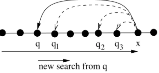
q x
new search from q q1 q2 q3
Fig. 3.Amortized complexity of the forward search. The search starts again from q. On this instance l = 3 and q + 3 < x.
The important point to notice is that after having identified the right back-ward transition from x for ti+1 reaching state q (there must be one), the search
for ti+2starts from q < x. Moreover, we associate all l transitions qk= δk(x, [i, j])
touched before finding the right one to its ending state which verifies q < qk< x.
Thus q + ` < x. This point is illustrated in Figure 3. As the search starts again from q and that at most one forward transition is passed through by text sym-bol, the total number of forward and backward transitions touched or passed through when reading the whole text t = t1. . . tn is thus bounded by 2n. ut
.
Proof (Proof of lemma 3). . Exactly as in the case of a classical text, we amortize the complexity of the search over the number of transitions we pass through and the number of reinitialisations of the search we do if no more failure transition is available. Each time we pass through a failure transition, we decrease the state from where we will go on the search if the state is validated. Thus, there can be at most as many failure transitions passed through during the whole reading of the text as the number of forward transitions that has been passed through. Since this number is at most the size of the text, the total number of transitions touched is at most 2n. Then, if after a descent from failure transition to failure transition no more outgoing transition exists, we reinitialise the search to state
1. Thus there are at most n such reinitialisations and the total complexity of transitions and states touched is bounded by 3n. ut
.
Proof (Of Lemma 4). Before processing, the pattern we first reduce the range of the keys from [n] to [m]. This is done in deterministic O(m log log m) times by first sorting the keys using the fastest integer sorting algorithm due to Han [8], and then replacing each key by its rank obtained from the sorting.
We then process the pattern in left-to-right in m steps and at each step j determine the failure and forward transitions outgoing of state j. We use two predecessor data structures that require O(m) words of space and support insert, delete and query operations (a query operation returns both the predecessor and the successor) in (worst-case) time O(log log m). As we move forward in the pattern, we insert each symbol in both predecessor data structures (except for the first symbol which is only inserted in the first predecessor data structure). The difference between the two predecessor data structures is that the first one will only get insertions while the second one can also get deletions. The first is used to determine forward transitions while the second one is used to determine failure transitions.
We now show how we determine the transitions at each step j. The forward transitions connecting state j to state j + 1 is labeled by rep(p, j + 1). The latter is determined by doing a predecessor search for pj+1 on the first predecessor
data structure. This gives us both the predecessor and successor of pj+1 among
p1. . . pj which is exactly rep(p, j + 1).
The failure transition is determined in the following way. If the target state of the failure transitions of state j− 1 is state i. Then we do a predecessor query on the the second predecessor data structure. If the pair of returned prefixes is precisely rep(p, i + 1), then we can make i + 1 as a target for state j. Otherwise we take the failure transition of state j− 1. If that transitions leads to a state k, then we remove the symbols pj−i..pj−k from the second predecessor data
structure. ut
.
Proof (Of Property 3). We first build the Morris-Pratt representation in O(m log log m) time. We then consider each state x > 0 corresponding to the p1. . . px from left
to right and for each such state we expand its backward transitions. Let us sort all pi, 1 i x and consider the resulting order pi0 = −1 < pi1 < . . . <
excepted if pij+1 = pij + 1. This transition is computed as follows. Let q be
the image state of the failure transition from x. We pick a value z in [pij, pij+1]
an search for z from q. Let q0 be the new state reached. We create a backward
transition form x to q0 labeled [pi
j, pij+1]. After this process we created at most
m2 edges in at most O(m2log log m) time.
We now merge backward transitions from the same state to the same state that are labeled by consecutive intervals. This required at most O(m2) time.
The whole algorithm thus requires O(m2log log m) time. ut
.
Proof (Of Theorem 3). We now give the details of the construction of the failure transitions in the AC automaton. The construction of the forward transitions has already been explained in section 4.
In order to build the failure transitions we decompose the trie into r layers. The first layer consists in the nodes of the trie that represent prefixes of length 1. The second layer consist in all the nodes that represent prefixes of length 2, etc.
Next, we will reuse the same algorithm that was used in 4 to build theMP automaton but adapted to work on the AC automaton. However, instead of using a single predecessor data structure we will use multiple predecessor data structures and attach a pointer to a predecessor data structure at each trie node. A node of the original non compacted trie will share the same predecessor with its parent, iff it is the only child of its parent. The following building phases will no longer reuse the normalized patterns, but instead reuse the original patterns. To each node, we attach a pointer to one of the original patterns. More precisely if a node has a single child, then his pattern pointer will be the same as its (only) child pattern pointer. If a node has more than one child (in which case it is called a branching node), then it will point to the shortest pattern in its subtree. If a node is a leaf then it will directly point to the corresponding pattern. A predecessor data structure of a node whose pattern pointer points to a pattern of length u will have capacity to hold u keys from universe u and thus will use O(u) space. This is justified by the fact that the predecessor data structure will only hold at most u elements of the patterns and each element value is at most u (recall that the pattern is a permutation of length u).
In order to bound the total number of predecessor data structures and their total size, we consider a compacted version of the trie (Patricia trie), where each node with a single child is merged with that single child. A node in the original (non-compacted) trie with two of more children is called branching node. It is clear that the set of nodes of a patricia (compacted) trie are precisely the branching nodes and the leaves of the original trie.
It is a well known fact that a Patricia trie with r leaves has at most 2r− 1 nodes in total. Thus the total number of predecessor data structures will be upper
bounded by 2r− 1. During the building if a node at layer t has a single child, then that single child at level t + 1 will inherit the predecessor data structure of its parent. Otherwise if the node v at level t has two or more children at level t + 1, then a predecessor data structure is created for each child u. Then if the predecessor data structure of v contains exactly k elements, those elements are precisely xt+1−k. . . xt, where x is string pointed by v. We will insert the k
elements yt+1−k. . . ytinto the predecessor data structure of u, where y the string
pointed by u.
In order to bound the total space used by the predecessor data structures, we notice that the total capacities of all predecessor data structures is O(m). This can easily be proved. Because we know that the total length of all patterns is bounded by m, we will also know that the total cumulative length of all strings pointed by branching node is also upper bounded by m. This is because precisely the pointed strings are precisely the shortest strings in the subtrees rooted by the branching node. The same holds for the leaves as the capacities of their respective predecessor data structures will be no more than the total length of the patterns that correspond to the leaves which is O(m).
We finally need to bound the total construction time which is dominated by the operations on the predecessor data structures. The time is clearly bounded by O(m log log r). This is by a straightforward argument: as the total sum of the pointed strings is O(m), and we know that each element of a pointed string can only be inserted or deleted once, and furthermore each insert/delete cost precisely O(log log r) worst-case time, we conclude that the total time spent in the predecessor data structure is worst case O(m log log r). ut
.
Proof (Of Lemma 5). Let A be an algorithm to search for p in t running in O(l) time. It can be converted in an algorithm to search for p inside all si(t)
also running in O(t) since: (a) it suffices to remove all occurrences overlapping two segments and occurrences in the last few remaining symbols of t out of a segment; and (b) in O(l) time, only at most O(l) such occurrences can be reported, so only O(l) occurrences might have to be discarded; and (c) testing if an occurrence is overlapping two segments can be done in constant O(l) time. The extra work required to remove all overlapping occurrences is therefore also O(l), and thus A can be converted in an O(l) algorithm to search for p inside all segments si(t). This implies that a lower bound for this last problem is also
a lower bound for A.
Proof (Of Lemma 6). All segments si(t) are identically distributed,
indepen-dently of each other. Thus the average time for searching for p in any segment is the same. As the expected time is the sum of the expected time to search for p in all segments, the sum commutes and the expected time becomesbn/(2m−1)c times the average expected time to search for p in any segment. ut
.
Proof (Of Lemma 7). Let 1 i1 < i2. . . < i` m be the position of the
accesses. For 0 j d, we define
Bj ={b | b 2 {1, 2, . . . , m} and j + b = itfor some 1 t `} .
Note that|Bj| ` for 1 j d. Also, for any p 2 Pm(`), since it is canceled by
the ` accesses considering isomorphic orders, for all shift j there is a mismatch, i.e. there exists two positions k, ` 2 Bj such that p[k] > p[`] and t[j + k] <
t[j + `]. We then show that we can find J ⇢ {0, 1, . . . , d}, |J| =⌃d/`2⌥, such that
Bj1\ Bj2 =; for j16= j2in J.
We use a greedy procedure to find J. Let j1 = 0. Inductively, suppose that
we have found j1. . . jk−1. Then jk is obtained by finding the smallest j such
that Bj is disjoint from the unions of the previous positions we have already
chosen, namely B = Bj1[ Bj2[ . . . Bjk1. We claim that this procedure allows us
to find at least⌃d/`2⌥ such sets. We prove in fact that j
k `2(k− 1) as long as
`2(k− 1) d. Observe that B contains at most `(s − 1) positions. We thus claim
that at least one of the sets inF = {B0, B1, . . . , B`2(s−1)} is disjoint from B. If
not, for each r, 0 r `2(s
− 1) there exists a pair (b, it) such that b2 Br\ B
and r + b = itfor some 1 t `. So there must exists at least `2(s− 1) + 1 such
pairs, one for each set Br. But the total number of such pair is no more than
|B| · ` `2(s
− 1), a contradiction.
Now take J⇢ {0, 1, . . . , d}, |J| =⌃d/`2⌥, such that B
j1\ Bj2 =; for j16= j2
in J. To prove the lemma, consider a random pattern p from Sm (the set of
permutations of size m). Then for all shift j2 {0 . . . d}, there is a mismatch. So P (p2 Pm( )) = P (8j 2 {1 . . . d}, there is a mismatch)
P (8j 2 J, there is a mismatch).
Notice that for each j2 {1 . . . d}, the probability that there is no mismatch with p at shift j is 1
|Bj|! which is the probability that the permutation formed by the
non-? symbol is the good one. Since all the sets Bj for j 2 J are disjoints, we
have
P (p2 Pm(`))
Y
j2J
P (there is a mismatch at shift j)
Y j2J (1− 1 |Bj|! ) ✓ 1− 1 `! ◆d`2de
concluding the proof since|Sm| = m! . ut
.
Here we prove that ` = log log mb log m with some b = 1 + o(1) verify the following inequalities for m large enough:⌃m−1
`2 ⌥ ⇥ 1 `! 1/10 (ineq.1) and 195 200 1 − ⇠ m − 1 `2 ⇡ ⇥`!1 10099 .
Let’s recall that the Gamma function of Euler Γ is an increasing bijection from R≥2 to R≥1 verifying that Γ (n + 1) = n! for all n2 N.
Thus the function s7! s2Γ (s + 1) is an increasing bijection from R
≥1 to R≥1.
For all m≥ 1, this allows to define s 2 R≥1 such that s2Γ (s + 1) = 50m.
Thus s! 1 when m ! 1. Then we set b = s⇥log log mlog m .
Taking ` = s, then we have ` =log log mb log m .
Let us prove that ` satisfied the desired inequalities.
We have `2⇥ `! = s2Γ (s + 1) = 50m. Thus ⌃m−1 `2 ⌥ ⇥ 1 `! m 50m 1 50 and ⌃m−1 `2 ⌥ ⇥ 1 `! ≥ m−150m ≥ 1 100 for m large
enough. This proves the desired inequalities since 1/50 1/40 = 1 − 195/200 1/10.
Let us prove now that b = 1 + o(1).
By the Stirling inequality, we have that F (s) < Γ (s + 1) < 2F (s) with F (s) =%s
e
&sp 2⇡s.
Thusp2⇡ exp(G(s)) < s2Γ (s + 1) < 2p2⇡ exp(G(s))
with G(s) =−s +%s +5 2& log(s). We deduce that p25m 2⇡ < exp(G(s)) < 50m p 2⇡. Therefore log⇣p25 2⇡ ⌘ + log m < G(s) < log⇣p50 2⇡ ⌘ + log m.
Recall that f (m)⇠ g(m) means that f(m) = g(m) + o(g(m)) when m ! 1. Thus we have G(s)⇠ log m.
It is then enough to prove that G(s)⇠ b log m. Indeed this imply b ⇠ 1, i.e., b = 1 + o(1).
But G(s) =−s +%s +5
2& log(s) = s log s + o(s log s).
Thus s = o(G(s)), i.e., s = o(log m).
Since s =log log mb log m , this means that b = o(log log m)
Moreover log s = log b + log log m− log log log m = log log m + o(log log m). As G(s) =−s +%s +5
2& log(s) we then have:
G(s) =−log log mb log m +
⇣ b log m
log log m+ 5 2
⌘ ⇣
log log m + o(log log m)⌘. Thus G(s)⇠ b log m, concluding the proof.