HAL Id: hal-01829241
https://hal.archives-ouvertes.fr/hal-01829241
Submitted on 3 Jul 2018
HAL is a multi-disciplinary open access
archive for the deposit and dissemination of
sci-entific research documents, whether they are
pub-lished or not. The documents may come from
teaching and research institutions in France or
abroad, or from public or private research centers.
L’archive ouverte pluridisciplinaire HAL, est
destinée au dépôt et à la diffusion de documents
scientifiques de niveau recherche, publiés ou non,
émanant des établissements d’enseignement et de
recherche français ou étrangers, des laboratoires
publics ou privés.
gravity and light sensing
Laurent Duchemin, Christophe Eloy, Eric Badel, Bruno Moulia
To cite this version:
Laurent Duchemin, Christophe Eloy, Eric Badel, Bruno Moulia. Tree crowns grow into self-similar
shapes controlled by gravity and light sensing. Journal of the Royal Society Interface, the Royal
Society, 2018, 15 (142), 10 p. �10.1098/rsif.2017.0976�. �hal-01829241�
Version postprint
Laurent Duchemin and Christophe Eloy
Aix Marseille Univ, CNRS, Centrale Marseille, IRPHE, Marseille, France
Eric Badel and Bruno Moulia
UCA, INRA, UMR PIAF, F-63000 Clermont-Ferrand, France (Dated: April 27, 2018)
Plants have developed different tropisms: in particular, they re-orient the growth of their branches towards light (phototropism) or upwards (gravitropism). How these tropisms affect the shape of a tree crown remains unanswered. We address this question by developing a propagating front model of tree growth. This model being length-free, it leads to self-similar solutions, independent of the initial conditions, at long time. Varying the intensities of each tropism, different self-similar shapes emerge, including singular ones. Interestingly, these shapes bear similarities with existing tree species. It is concluded that the core of specific crown shapes in trees relies on the balance between tropisms.
I. INTRODUCTION
In many tree species the outer shape of the crown is a cri-terion for species identification, especially when trees have grown in isolation. The Mediterranean cypress has a dis-tinctive elongated shape, while birch and oaks show more spherical shapes, and the Norway spruce has a conical pro-file. The growth process that leads to these different silhou-ettes is not well understood. It is associated with genetically fixed species-dependent factors like the branching angles, the phyllotaxy, and more generally the developmental character-istics of the branching architecture known as the “architec-tural model” of the species [1]. But crown shapes are also af-fected by the environmental growth conditions (in a genetic-dependent manner): trees grow differently if they are isolated or in a forest [2], if subject to climatic stresses like wind or snow cover [3]. So far, the few studies about crown shaping have investigated the hypothesis that it may result from an interplay between a genetically-defined architectural devel-opment and branch growth or shedding linked to light com-petition [4].
However tropisms in the outer growing branches can be viewed as another possible candidate for the control of crown shape. Tropisms are defined as the re-orientation of a grow-ing branch followgrow-ing a vectorial cue from the environment. Two tropisms are shared by most plants: phototropism is the process that leads to growth in the direction of light, while gravitropism is driven by the direction of earth gravity. Ge-netic differences in tropic sensitivities have been reported [5, 6]. The study of these tropisms is still an active field today, ranging from shoot scale [6–9], to the molecular networks that regulate them [10]. Yet, a question remains largely open: how do these tropisms and their balance influence the shape of a tree crown?
In this work we investigate the simple hypothesis that the two tropisms of the peripheral primary shoots at the tip of the branches can be major players in driving the shaping of the crown, accounting for the interplay between genetic con-trol and responses to the local environment. To do so we developed a simple model of the crown growth. In the lit-erature, popular growth models generally consider branches
and leaves as the elementary bricks of a numerical simula-tion [11–15]. However these models usually involve a large number of empirical parameters, and thus remain too com-plex to study the specific roles of phototropism and gravit-ropism in selecting the tree shapes. Recently, Beyer[16] pro-posed a simpler and more parsimonious model that consid-ers the whole tree as a continuous medium. This approach seems very promising, but has not yet been fully exploited to address the combined role of phototropism and gravit-ropism. In this Letter, we propose a new idea: considering the growth of a tree crown as a continuous front propagation process. Despite some similarities with other front propaga-tion processes, such as crystal growth [17], premixed com-bustion [18], or Saffman–Taylor fingering [19], tree growth has some distinctive features.
In particular, since growth involves photosynthesis and is controlled through light sensing (photomorphogenesis), our model includes both photosensitivity (the foliage receiving more light will grow faster), phototropism (growth is pref-erentially oriented in the direction of light), and also gravit-ropism (growth is preferentially oriented against gravity). As we shall see below, the proposed model requires only two pa-rameters to describe the shape of the crown (irrespective of its size): the intensities of phototropic and gravitropic grow-ing responses. With this model, we intend to address the following questions: What is the family of shapes generated when these two parameters vary? Do these shapes converge towards steady solutions? How these steady solutions can be described analytically? And finally do these solutions fit the major classes of crown shapes observed in undisturbed isolated trees in nature?
II. CROWN GROWTH MODEL
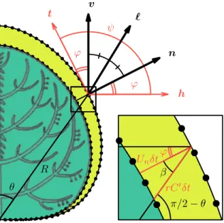
We first assume that the average sunlight is uniformly dis-tributed in the upper hemisphere, but we shall come back to this strong assumption in the discussion section. When the crown envelope is convex and axisymmetric, the amount of light received daily at each point of the front is thus assumed to be proportional to ψ , the angle between the local tangent and the horizontal (Fig. 1). At each point on the front, n
Version postprint
resents the outward normal unit vector, ` is the unit vector that represents the average direction of light, v is the upward vertical unit vector, and κ is the in-plane curvature, positive when the surface is locally concave (Fig. 1). According to this nomenclature, the velocity of the front is written as
U = ψ n+ αдv+ αp` n+ αдv+ αp`
+ γκn, (1) where αдand αpare the intensities of the crown gravitropic
and phototropic responses respectively, and γ is similar to a “surface tension”, but acting on the growth velocity.
n ` v ϕ ϕ ψ h t θ R Unδt rC0δt π/2− θ ϕ β
Figure 1. Sketch of a growing tree crown. h and v are unit hori-zontal and vertical vectors respectively, n and t are the unit vectors respectively normal and tangent to the front and the unit vector ` points towards the mean direction of light, which is the first bisec-tor of (h, t). The angle ψ = φ + π/2 represents the local amount of sunlight intercepted for this axisymmetric shape. The inset shows a zoom around the front to highlight the conditions for self-similarity of the growing shape.
Our model is based on two basic assumptions: [A1] the crown foliage is dense enough all across the crown so that it may be described as a continuous medium with a continu-ous boundary line (i.e., a growth front); [A2] all the growing apices sitting on the front have similar dependency on light and gravity. Assumption [A1] requires that the development of the tree crown is sufficient and the crown displays a steady characteristic shape, a condition that is usually observed in most species as soon as they have reached the “architectural unit” (AU) stage, i.e. that they have differentiated all their branch types [20]. [A2] requires that “rogue branches” do not occur. It is well known that traumatic reiteration result-ing from branch accidental breakage or from large herbivory damages produces re-juvenilised branches that behave dif-ferently than regular branches (e.g., suckers). These trau-matic reiterations should be distinguished from regular re-iterations involved in the process of crown morphogenesis (a
process known as branch metamorphosis [1, 20]), as these re-iterated branches still complie with a regular behaviour and the crown remains dense.
The first term on the right-hand-side of Eq. (1) includes two important biological mechanisms. First, the front velocity is assumed to be proportional to ψ , the light intercepted, to ac-count for photosensitive growth. Second, the gravitropism and the phototropism are modelled through a re-orientation of the growth in a direction computed as the weighted aver-age of the three unit vectors n, v, and `. This modelling of tropisms is in accordance with the experimental observations made at the level of a single shoot, and with the ArC model of shoot gravi-photo-tropism, that was assessed against exper-iments [21]. Additionally, it has been demonstrated experi-mentally that the sensitivity to the gravity is not dependent on the angle made by the shoot versus gravity. The mech-anism subtending this behaviour lies in the functioning of specialized cells called statocytes (see [6, 7, 22, 23] for more explanations on the physics and biology behind this mecha-nism). For phototropism, the equation and the definition of phototropic sensitivity are mainly similar (see [21] and ref-erences therein).
The last term in Eq. (1) stabilises the front dynamics and smoothes out the front shape by damping the velocity fluc-tuations, and hence has a similar role as surface tension in Saffman–Taylor dynamics for example. There is obvi-ously no surface tension acting at the boundary of the tree crown. However recent ecophysiological investigations have revealed that two biological mechanisms are acting as to re-duce the differences in growth velocities of neighbouring shoots, and hence resulting in a flattening tendency of the canopy boundary, which is qualitatively similar to a surface tension. The first mechanism is due to lateral sensing of the spectral signature of the light reflected by neighbouring plants, through the phytochrome pigment [24]. This sens-ing results in a photomorphogenetic synchronisation of the growth in length of the neighbouring stems, keeping the top of the canopy flat. The second mechanism involves the sens-ing of wind-induced strains [25]. Whenever a shoot over-reach its neighbours, it is not sheltered by the canopy any-more and its growth speed is reduced until the front is flat again. It has been shown nicely in herbaceous populations of shoots that these two mechanisms are responsible for the flat-tening tendency of canopy tops, as dramatically illustrated by the flatness of the top surface of crops such as wheat or corn [26]. On a practical point of view, when simulating the growth of a crown, we rescale its shape at each time-step to keep its axi-symmetric volume V constant. As explained in the next section, this is equivalent to a coefficient γ grow-ing in time in Eq. (1). Although this rescalgrow-ing may seem un-physiological, we perform it for two reasons: it ensures that the code is stable at long times, and it allows to reach self-similarity (when surface tension is rescaled, Eq. (1) has no length scale and self-similar solutions emerge).
Finally it may be noted that in our simplified model, the curvature κ is calculated in a vertical plane, and not as the three-dimensional mean curvature of the axisymmetric in-terface. The latter refinement would be possible, but does
Version postprint
(a) (b)
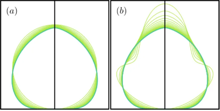
Figure 2. Superimposed views of a tree crown growth for two dif-ferent initial conditions. In (a) the initial shape is a circle and in (b) a circle with a significant O(1) perturbation. Parameters are: αд = αp = 0 and γ = 0.01. The light green curves correspond
to different instants. The dark green curves correspond to the self-similar solution at large time. The shape is rescaled at each time-step in order to keep its volume constant equal to one.
not affect the main features of the solutions.
III. NUMERICAL SOLUTIONS
Equation (1) is solved numerically by placing N = 200 marker points on the front. The points are then advected along the normal to the front. Furthermore, at each time-step, the coordinates of the front are rescaled by the volume to the power 1/3, such that the crown volume remains constant (V = 1). This rescaling makes the problem scale-invariant and allows the “surface tension” to remain of the same order during the growth process. As a consequence, the scaling of the true curvature in the physical plane increases like V1/3.
Since the “surface tension” coefficient in the numerical space γ∗is kept constant, it means that :
γ = γ∗V1/3. (2) Since V = 1, we can drop the star and use γ in place of the constant γ∗.
The surface points are advected in time using an explicit second-order scheme [27], with a time-step δt ∼ δs2/γ,
where δs is the typical distance between two successive marker points, chosen to ensure the stability of this explicit scheme. The markers are redistributed on the front at each time-step, in order to conserve a regular spacing. Note that the “surface tension” becomes significant when γκ ∼ O(1), as seen in Eq. (1).
Figure 2 shows two examples of such a computation for two distinct initial conditions. In this example, there is no phototropism and no gravitropism (αд= αp= 0) and surface
tension is set toγ = 0.01, small compared to the global length scale: γ 1.
We first observe that, although initial conditions signif-icantly differ, the successive shapes converge towards a unique self-similar shape (Fig. 2a). This self-similarity was expected because the problem has been made scale-invariant.
To further test this idea, we performed extensive numerical simulations with different parameter sets (αд, αp), at low
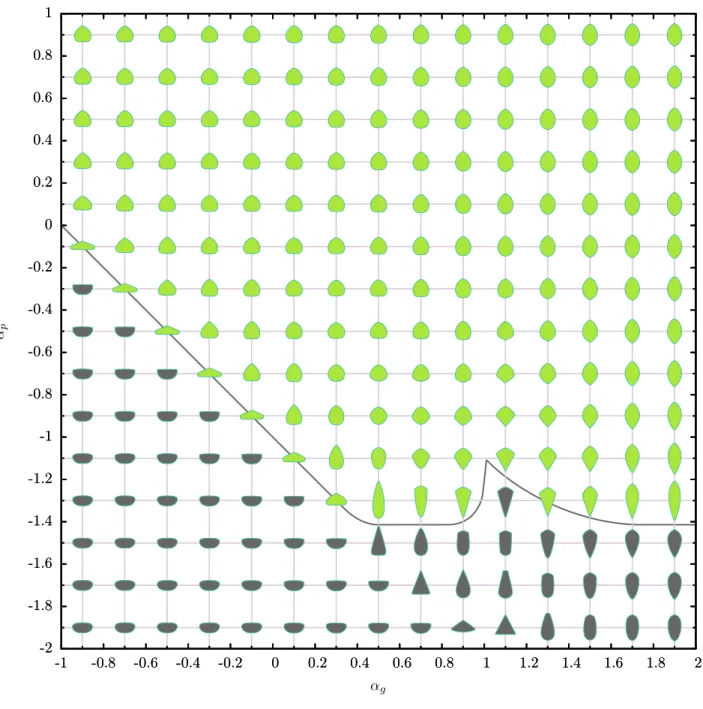
sur-face tension (γ = 0.01). The results are presented in fig-ure 3: green shapes correspond to computations that have converged towards self-similar shapes, meaning that a typi-cal distance between two successive restypi-caled shapes (Fréchet distance) has reached 10−6, whereas grey shapes correspond
to non-convergent computations (in these cases found in the lower-left part of the diagram , the shape flattens out indef-initely and convergence is never reached). The grey curve which segregates converged from non-converged shapes will be discussed in section V.Figure 3 displays a large diver-sity of shapes as a function of the parameter sets (αд, αp),
showing that the (genetic) variation in the sensitivities to phototropism and gravitropism can indeed produce different crown shapes in our model.
Moreover, we performed numerical simulations with de-creasing surface tension γ (Fig. 4). The results showed that all the final self-similar shapes converge towards a universal shape in the limit γ → 0. In the next section, we focus on this limit and show that this universal shape can be derived analytically, providing insight into the control of the steady-state crown shape, when it exists, by the parameter sets (αд,
αp).
IV. ANALYTICAL SOLUTIONS
In the limit of vanishing surface tension (i.e. γ → 0), Eq. (1) becomes scale invariant. We look for a self-similar solution of this equation by imposing that the front is described by the homothetic surface:
R(θ , ϕ, t )= r(θ)C(t), (3) in spherical coordinates (Fig. 1).
Between two successive times, t and t + δt, the front has been increased by r(θ)C0
(t )δt in the radial direction. This condition can be expressed as
r (θ )C0(t )δtcos β = U · n δt = ψB(φ) δt, (4) where ψ = φ + π/2, β = π/2 − θ − φ and B(φ)= n+ αдv+ αp` n+ αдv+ αp` ·n. (5) To solve this problem, we first note that cones are triv-ial self-similar solutions of Eq. (4), with φ the constant angle between the cone surface and the vertical direction (Fig. 1). Moreover, Eq. (4) implies that C0
(t )does not depend on time. The cones having the same velocity C0(that we choose equal
to 1 without loss of generality) intersect the vertical axis at the elevation
zc(φ)= r(0) = (φ + π/2)B(φ)/sin φ. (6)
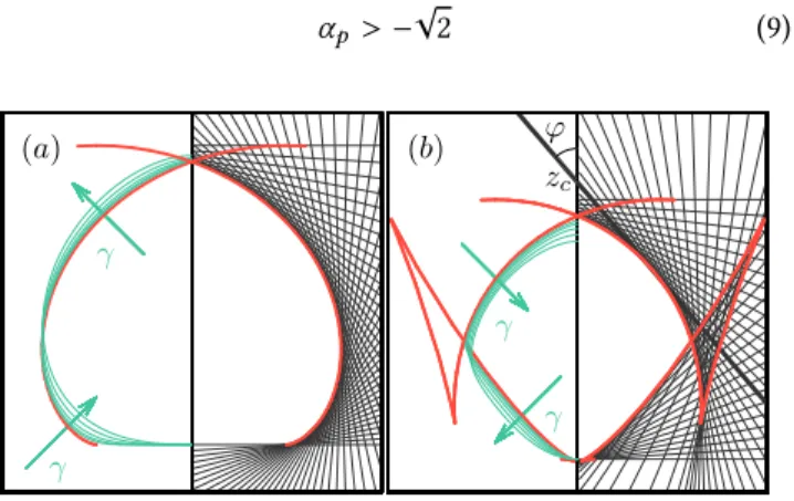
Figure 4 shows the cones described by Eq. (6) for two dif-ferent sets of parameters. The universal shape we found nu-merically in the limit of vanishing surface tension appears
Version postprint
-2 -1.8 -1.6 -1.4 -1.2 -1 -0.8 -0.6 -0.4 -0.2 0 0.2 0.4 0.6 0.8 1 -1 -0.8 -0.6 -0.4 -0.2 0 0.2 0.4 0.6 0.8 1 1.2 1.4 1.6 1.8 2 αp αg -2 -1.8 -1.6 -1.4 -1.2 -1 -0.8 -0.6 -0.4 -0.2 0 0.2 0.4 0.6 0.8 1 -1 -0.8 -0.6 -0.4 -0.2 0 0.2 0.4 0.6 0.8 1 1.2 1.4 1.6 1.8 2Figure 3. A set of crown shapes obtained from a numerical computation, varying αд and αp, and with γ = 0.01. Green shapes have
converged towards a self-similar-one, whereas grey shapes have not converged. For each shape, the parameter values correspond to the grid intersection.
as the inside envelope of all those cones. Interestingly, this inside envelope can be obtained analytically.
For convenience, we switch to cartesian coordinates. The cones of Eq. (6) intersect the plane y = 0 along the straight line described by the equation: z = zc(φ) − x/tan φ.
Conse-quently, two cones corresponding to angles φ and φ +δφ will
intersect at the point
x(φ)= −z0c(φ)sin2φ, (7)
z(φ)= zc(φ)+ zc0(φ)sin φ cos φ. (8)
When −π/2 ≤ φ ≤ π/2, Eqs. (7–8) describe the cone en-velope as a parametric curve (red curves in Fig. 4). Because this parametric curve is everywhere tangent to a cone with the same time evolution C(t), it is also a self-similar solution of Eq. (1) for γ = 0. This approach is similar to the Wulff
Version postprint
construction used in the physics of crystal growth [28, 29]. Another interesting feature of these self-similar shapes arises from following the trajectories of surface points back-ward in time. These trajectories can be thought of as traces of the underlying structure, i.e. the tree branches. Figure 6 shows these trajectories for two cases: αд = αp = 0 and
αд = αp = 2. These trajectories are numerically calculated
by advecting backward in time 31 points along the vector −U. At each time step, the points –lying on a smaller self-similar shape– are associated to an updated angle ψ using cubic splines. For αд = αp = 0, there is a region without
branches close to the bottom. This region is a consequence of the flat bottom, where ψ = 0 and the front velocity is zero. Note that the curvature of the “branches” is only due to the variation of ψ and ` along these trajectories, and not to the bending under self-weight of the branches or any other global orientating mechanisms such as those related to re-action wood[30], which are not taken into account in our model.
We will discuss below why numerical simulations con-verge towards the parametric solution given by Eqs. (7– 8). Meanwhile, we describe how the respective intensities of gravitropic and phototropic responses modify the crown propagation and the final shape.
V. COMPARISON BETWEEN NUMERICAL AND ANALYTICAL SOLUTIONS
We note that these attracting shapes do not exist for any choice of the parameters αд and αp, as already observed in
figure 3. Figure 5a shows with grey levels how fast the nu-merical solution converges towards a self-similar solution. It also shows that in the lower part of this diagram, there is no convergence. Equation (6) indicates the cases when self-similar shapes exist. The convergence occurs when the cone with a vertical angle (φ = 0) exists (i.e. x(0) > 0 in Eq. 7). This condition simplifies to:
αp > − √ 2 (9) γ γ γ γ zc (a) (b) ϕ
Figure 4. Attracting shapes obtained for different values of γ : γ = 0.04, 0.02, 0.01, 0.005 and 0.0025, with αд = αp = 0 (a) and αд =
0.8, αp= −1 (b). The envelope of the grey lines given by equation (6)
is the expected self-similar shape. When γ → 0, the time-evolving shapes converge towards this self-similar shape.
Moreover, the self-similar shapes cease to exist when their top (given by z0
c(φ) = 0, φ ∈ [0, π/2]) reaches their
bot-tom (z0
c(φ) = 0, φ ∈ [−π/2, 0]). This condition can be
computed numerically and corresponds to the light green curve in figure 5a. A good approximation of this curve for αд ∈ [−2,
√
2 − 1] can be obtained by writing that the self-similar shapes exist roughly when the two cones with hor-izontal angles (φ = ±π/2) are one above the other (i.e. zc(π /2) > zc(−π /2) in Eq. 6), a condition that simplifies to:
αp+ αд> −1 (10)
These existence conditions correspond to the light green curve in the phase diagram (Fig. 5), below which there is no analytical self-similar solution. The curve is also reproduced in figure 3 and is perfectly consistent with the convergence region observed for the time-evolving shapes.
When they exist, self-similar solutions exhibit different characteristics that correspond to different hatchings in Fig. 5a. First, we note that the self-similar solutions always feature a pointed top. It happens for z0
c(π /2) > 0, with zc
given by Eq. (6). This condition is equivalent to αp+αд> −1;
which is guaranteed by Eq. (10).
Second, the self-similar shape can exhibit a pointed bottom when z0
c(−π /2) > 0, or equivalently when x(−π/2) < 0. This
configuration is equivalent to αд > 1 (dark green hatching
on the right of Fig. 5a). Examples of such shapes are dis-played in Figs. 5c,i,j. Note that, contrary to flat-bottomed shapes (Figs. 5b,e,g, for instance), these shapes have a non zero growth velocity at their pointed bottom.
Third, the bottom of the self-similar shape can present a cusp when x0(−π /2) ≤ 0; which is equivalent to α
p(2αд2 −
2αд+ αp2) ≤0 (red hatching in Fig. 5a). This cusp can clearly
be seen in the self-similar solutions displayed in Figs 5i,j where the value of x at the bottom (for φ = −π/2) initially decreases. The same cusp is also perceptible in Figs 5d,g,h, although it is less pronounced.
Finally, the self-similar shape described by the paramet-ric curve given in Eqs. (7–8) can exhibit a loop, as seen in Figs. 5h,i (it is also perceptible in Fig. 5f, but less visible). This loop corresponds to the zone with the yellow hatching in Fig. 5a, whose boundary has been determined numerically. As seen in Figs. 4 and 5b–i, the numerical self-similar so-lutions obtained at long time always converge, in the limit of vanishing surface tension, towards the inward envelope of the cone solutions given by the parametric curve of Eqs. (7– 8). However, when surface tension is zero, any shape con-structed as an assembly of pieces of cones could be a valid self-similar solution. These solutions do not occur in the nu-merical simulations for two reasons: first, any connection between two pieces of cones tend to “recess” towards the in-ward envelope when the surface tension is non zero. Second, the front propagation is described as the advection of markers in the direction normal to the front, whereas a special numer-ical treatment of the corners would be necessary to maintain a solution made of several assembled cones.
Version postprint
-2 -1 0 1 2 3 -2 -1 0 1 2 3 -2 -1 0 1 2 3 -2 -1 0 1 2 3 -2 -1 0 1 2 3 -2 -1 0 1 2 3 -2 -1 0 1 2 3 -2 -1 0 1 2 3 -2 -1 0 1 2 3 -2 -1 0 1 2 3 -2 -1 0 1 2 3 -2 -1 0 1 2 3 In tensit y of phototropic resp onse αpIntensity of gravitropic response αg
j c b g e f h i d (a) (b) (c) (d) (e) (f ) (g) (h) (i) (j)
Figure 5. (a) Phase diagram in the αд–αpplane. The grey level is proportional to the number of time-steps necessary for convergence towards
a self-similar shape (black corresponds to no convergence). The hatchings correspond to different features of the self-similar shapes: light green for no self-similar solutions, red when a cusp is present at the bottom, yellow for a loop, and dark green for a pointed bottom (more details in the main text). The white square corresponds to figure 3. (b–j) Characteristic shapes found numerically for γ = 0.01 (green curve and fill) and analytically in the limit of vanishing surface tension with Eqs. (7–8) (red curve). The thin black lines correspond to the vertical symmetry axis (Oz) and to the horizontal plane z = 0. Shapes (i) and (j) have been rescaled by a factor of 2 in both directions, whereas all others shapes have the same volume.
Figure 6. Trajectories of points along the front, for the cases αд =
αp= 0 (left) and αд= αp= 2 (right). Starting from the self-similar
profile corresponding to t = 1, 31 points are advected backward in time using Eq. (1) until t = 0.1.
VI. COMPARISON WITH OBSERVED CROWN SHAPES
Care should be taken when comparing the predictions of the model with real tree crowns observed in nature. Indeed the impinging of light rays on the crown should not be in-tercepted by a neighbouring object (wall, rock, other trees). Moreover tree shoot should not be able to sense the reflected light from neighbouring crowns even in the absence of di-rect shading of the incident light. The few studies about the
distance of neighbouring sensing is limited to approximately 5 m [31]. Finally no external action such as pruning, grazing or wind-break should have occurred (at least at a scale that could affect the growth and shaping of the crown).
Another important aspect is that the external growing shoots should have a similar physiological and developmen-tal status. Indeed some reiterations (especially traumatic ones) can result in obvious disruptions of the regularity of the crown shape. Therefore, only two developmental stages were retained: (i) young trees approaching the “architectural unit stage” and (ii) mature trees having developed their scaf-fold limbs through the process of developmental metamor-phosis [1, 20].
We used two sources of tree crown pictures. The first source is an arboretum (E. Badel’s park, sitting in southern France in a sub-Mediterranean climate at 44.904°N, 4.830°E) where no pruning or grazing has ever been achieved and trees were planted at large distances from each other. The second source results from a search on botanical websites and Wikimedia Commons (https://commons.wikimedia.org), retaining only photographs for which the species and the lo-cation were known and the criteria concerning the absence of significant neighbours or traumatic reiteration could be assessed.
For each picture, the best fit is found using the following method. First, the right half part of the tree crown is de-scribed as a series of hand-picked points (typically about 20
Version postprint
(a) (b)
(c)
(c) (d)(d)
Figure 7. Comparison between real tree crowns and self-similar shapes of the model: (a): Betula pubescens, αд= 0.927, αp= 0.267, d = 0.022;
(b): Quercus castaneifolia, αд = −1.00, αp = 0.353, d = 0.019; (c): Enterolobium cyclocarpum, αд = −0.490, αp = −0.488, d = 0.023 (black
curve: αд = −1.00, αp = 0.034, d = 0.020), (d): Thuja occidentalis, αд = 0.379, αp = −1.23, d = 0.018 (black curve: αд = 5.00, αp = 2.69,
d= 0.079). The red curve represents the best fit and the black curve the best fit with αp> 0. See Supplementary materials for comparisons
with other tree species.
points). Then, we assume that the shape is axisymmetric and we rescale and shift this shape such that its volume is equal to unity and its center of mass is at the origin. After that, we look for the parametric curve described by Eqs. (7–8) that minimises the distance with the real tree crown, where the distance d is defined as d2= 1 π ∫ π 0 (Rmodel(θ ) − Rcrown(θ )) 2dθ , (11)
with Rmodeland Rcrownthe polar representations of the model
and tree crown respectively. This procedure allows to find the best parameters αд and αp. The same procedure is
re-peated with the additional constraint αp > 0.
This fitting method has been applied to 36 different tree crown pictures (see Supplementary Materials), out of which four representative cases have been extracted (figure 7). In figure 7a, the fit is fair with parametric values of αд and
Version postprint
αp both positive, as expected from what is known about
shoot tropisms, namely upward gravitropism and positive phototropism. For some trees, the shape of the crown could not be well fitted with positive values of αд and αp.
How-ever, allowing a negative value for αд(figure 7b) or αp(figure
7c,d), leads to a good fit. Negative values for αpwould mean a
negative shoot phototropism, a condition that is usually not observed in studies about shoot phototropism. We analyse in the discussion section the biological insights that such a situation may provide. Figure 7(c) and (d) provide two sets of parameters: the first one (red profile) for which we allowed any values for αp, the second one (black profile) for which αp
is constrained to be positive. These two comparisons clearly show that in some cases, like (c), the crown shape can be well fitted using several parameter sets (possibly even a contin-uum set of parameters), whereas others show a poor compar-ison with the real shape when αp is constrained to be
posi-tive. On this matter, the diagonal described by equation (10) and seen in figure 5 plays a particular role: close to this line, shapes look similar, allowing for a family of solutions.
VII. DISCUSSION
Many tree species display characteristic and heritable crown shapes, at least at some stages and when trees have grown in isolation. Yet crown shape is remarkably variable with the environment (what biologists call "platicity"): trees grow differently if they are isolated in full sunlight or in a forest[2], if they are submitted to wind or protected from it[3]... Reconciling these two features has remained a chal-lenge. Indeed there is a large number of biological mecha-nisms that can affect the intensity and orientation of shoot growth, e.g. phyllotaxis, apical dominance [1, 20], response of buds break to light[24], changes in growth directions at different developmental stages, tropisms, internal correla-tions between organs[1], as well as repulsive effects between branches mediated though phytochromes[24], biomechani-cal processes at the branch level, such as the bending of the branches under self-weight, its fixing through secondary growth and global orientating mechanisms related to re-action wood[30]. Moreover, the development of the crown is modifying the environment of the growing apices, creat-ing a feedback of the actual crown shape over its develop-ment (shading, wind sheltering...). All the challenge is then to identify the leading physical and physiological mechanisms which can explain the interaction between genetic control and sensitivity to the environment in the development of crown shape. Two standpoints can be adopted.
One is to concentrate on the development of the branched architecture through bud breaks, shoot growth, and its re-modelling through environmental factors interacting with the crown size and spread such as light competition or wind effects[4, 32]. The second stand-point is to concentrate on what is occurring at the boundary of the crown, and more specifically on the apical buds that are sitting on its vicinity, and which are responsible for the increment in crown spread through the annual flush of shoot growth. This standpoint
can be visualised when considering for example a coniferous tree in the springtime, on which the crown of the last year has kept its dark-green needles and the new sprouts undergoing primary growth (elongation) shows up with a much lighter green colour. The descriptive parameters of this crown in-crement are the distribution of the buds, the amount of their elongation, and their direction. And the interaction between the genetic specification and the local environment at the boundary of the crown is specified through the physiolog-ical processes that may influence these descriptive param-eters. This second standpoint is the one that has been in-vestigated in this work. Three different processes were thus retained: the photomorphogenetic photosensitivity of shoot elongation (referred to as photosensitivity) and the two major tropisms known to affect the direction of the primary growth: photo- and gravi-tropism[6, 21]. The initial orientation of the bud was considered to have negligible effect as growing shoot can reach their photo-gravitpropic set-point angle irre-spective of the original orientation in an interval of time that is very short compared to the morphogenesis of the crown shape (typically less than a day)[6, 21].
In this article, we model this process of incremental pri-mary growth at the boundary of the crown with a front propagation equation taking into account the effects of pho-tosensitivity, phototropism and gravitropism, and the feed-back of the actual crown shape through its shading effect of the growing apices, as a function of their position. We also included a synchronisation of the growth velocity among neighbouring shoots[24–26] resulting in a local flattening tendency of the canopy boundary, which is qualitatively sim-ilar to a surface tension. Through numerical simulations, we show that this front equation generally yields self-similar so-lutions at long time, independently of the initial shape. In the limit of vanishing surface tension, we show that these self-similar solutions can be described analytically by parametric curves, which, for particular values of the phototropic and gravitropic responses, can exhibit singularities.
The outputs of the model were then compared to real tree crowns. As the dynamics of the crown growth is at the core of the model, a direct comparison between the proposed front velocity, given by Eq. (1), and empirical observation of growth directions and amount would have been the best as-sessment. However, no such data was available, and their collection would require long term experiments. The assess-ment of the predictions of the model was thus achieved by comparing its self-similar solutions with real tree crowns at the special stages at which the crown displays a typical and stationary shape (namely the “architectural unit stage” and mature stages [1, 20]). This was achieved on 36 crown images of different tree species sampling many taxonomic clades from different climates. Using the distance d defined by Eq. (11) measuring how the shapes extracted from the pic-tures differ from the analytical parametric curves, we could find, for each picture, the set of phototropic and gravitropic intensities that best fit the tree crown. It appears that in 97% of the cases, we find a distance d < 0.05, which we consider as good (see Supplementary Materials).
Version postprint
about the values of the photo- and gravisensitivity param-eters; and the second one about the significance of the two important assumptions of the model (aside from the choice of the three mechanisms): the linear photosensitivity curve and the uniform lighting. Regarding the photo- and gravisensitiv-ity parameters, positive values of αpand αдallow for a
satis-factory comparison with real crown shapes in only 33% of the cases. For 75% of the cases, a reasonable fit can be obtained with the constraint αp ≥ 0. However negative values of αp
are required to fit the remaining 25% (figure 7d and Supple-mentary Materials). Negative shoot phototropism has never been documented in wild-type plants living in natural condi-tions and can be considered non-physiological. By the same token, negative shoot gravitropism is restrained to rare mu-tants, and is unlikely to be involved in the studied trees. How-ever, these negative values may reflect the influence of an-other tropism, namely auto-tropism[30]. Auto-tropism is the tendency for growing plant shoots to reduce their curvature, through a proprioceptive sensing[6, 33]. It was found that the proprioceptive auto-tropism is a major player of the orienta-tion of shoot growth[6, 21]. Auto-tropism was not included in our model and negative phototropism could compensate for that. But it could also compensate for other processes acting at the whole branch level (e.g, branch biomechanical reori-entation or shedding) that were not taken into account in the model. Some explicit representation of the growing shoot or of the whole branch would be required to asses if these additional mechanisms may account for the crown shapes that cannot be fitted with our model. Therefore a new re-search avenue emerging from the present work is to extend the model to account for the average orientation of branches along the crown boundary, the effect of, for example, auto-tropism, or self-weight [30] as well as some mechanisms of spatial competition[34] or of branch repulsion[24]. In this work we have assessed whether following the trajectories of surface points backward in time gives an idea of the under-lying branches structure. But effects such as auto-tropism or bending under self-weight were not taken into account in our model and the “inferred branch patterns” were clearly not very realistic.
The two other hypotheses of the model: i) linear photosen-sitivity of growth (the front velocity is assumed to be propor-tional to the average light intercepted) and ii) uniform light-ing (light, on average, is assumed to be uniformly distributed in the upper hemisphere) remain also to be discussed. In-deed, whereas the basis for the phototropic and gravitropic response lays on a wealth of published reports, as shown in the introduction section, the situation is less favourable here. Both hypotheses can be advocated to be a good starting point that allows to keep the model tractable and understandable (parsimony argument); yet they should not be ad hoc. The first hypothesis is grounded in the fact that plants have light sensors called phytochromes that allow them to be sensitive to the ratio between the Red light and the Far Red light (R:FR) [24]. FR light is almost fully reflected by foliage elements, whereas R light is largely absorbed. Then, for a finite front area A, the R:FR ratio can be well approximated by the ra-tio of visible sky and of visible surrounding foliage. When
A → 0, assuming that the density of surrounding foliage is uniform, this ratio remains proportional to the angle of visi-ble sky, and this corresponds to our model. In general it has been found that there is a linear relationship between the elongation rate of shoots and the R:FR ratio [24], which is usually negative for many open-habitat species (leading to a shade avoiding) and positive for some tree species (a behav-ior known as shade tolerance)[35]. The second hypothesis seems much less straightforward. It is only realistic for fully overcast skies on cloudy days. On sunny days, the diffuse light from the sky displays a fairly uniform radiance, but ob-viously the direct sunlight is highly non-uniform, with a bias towards the South (resp. North) in the Northern (resp. South-ern) hemisphere [36]. And including a direct sunlight com-ponent in our model would clearly break the axi-symmetry of the crown shape due to a faster growth in the sun-facing side. On the contrary, tree crowns in Nature do not seem to be biased towards the sun [37] (with the exception of Araucaria columnaris[38]). Is this a serious drawback for our model? Not necessarily. Indeed the phytochrome sensing of the R:FR ratio of the light is compensated for light intensity[24]. Be-sides the elongation growth is known to be impaired by wa-ter stress, that is related to the direct sunlight, so that higher growth may actually happen on overcast cloudy or rainy days, and hence under uniform lighting[39, 40]. Yet, to our knowledge, no explanation has ever been published to this puzzling question of crown axi-symmetry in isolated trees despite the asymmetry of many environmental factors (sun-light of course, but also evaporation, temperature...). But now that we have shown that the two previous assumptions cou-pled with phototropism and gravitropism led to realistically looking tree crown shapes, it is clear that investigating more thoroughly light-compensated sensing mechanisms and their relation to shoot growth and to crown shaping in trees is likely to be very rewarding. And including more mechanistic light responses in our model can be a tool to do so.
Despite this set of open points, our work clearly shows that the hypothesis that the observed crown shapes could be the result of a front propagation process driven by the light-and gravity- sensing at the crown boundary is a valid start-ing point. Moreover, it provides an insight on how to recon-cile the genetic specificity and the environmentally-driven variability (plasticity) of crown shapes. Indeed if a tree has enough time to reach a stationary shape, then there should be no more influence of the initial state and/or the pathway to this form. This stationary shape emerges from the recurrent effects of elongation photosensitivity and photo-and gravi-tropic sensitivities, and the feedback on these three processes of the interaction between the lighting environment and the actual crown shape. But the values of the three sensitivi-ties are genetically-fixed. This may explain how a process driven by three responses to the environment (and hence al-lowing plasticity) yields a steady-state form that is heritable and probably genetically controlled. The situation is simi-lar with what has been found for the shape of single shoots by[6, 21]. But for this to be achieved there should be no other player in the environment*crown shape interaction, a case only met when trees are grown in isolation and other
Version postprint
factors –e.g. shading by neighbours, wind, frost– are neg-ligible. It is likely not to be the whole story though. In-deed there are indications that the steady shapes of the same tree at the (young) “architectural unit stage” and at the ma-ture stage are different[1, 20] (although this does not rely on observations of the same tree at the two stages, grown in isolation). One may think that the shape control through photomorphogenetic and tropic mechanisms captured in our model only stabilises each of the two forms, whereas the shift between the two stages could be driven by changes in the branching development when trees developed their scaffold limbs through the process of developmental metamorphosis. To provide different attractors, though, non linear behaviour is required in our model; but there are many candidates for that (eg. interaction between different light sensors, phy-tochromes, cryptochromes[24]...).
However, before that, our work also points at the need for data following the development of isolated trees from differ-ent species during decades. Only this type of data may al-low to assess whether self-similarity is reached. Addition-ally the effect of minor interventions, such as partial prun-ing, could be studied experimentally by looking at the shape dynamics and relaxation towards a self-similar shape. Such detailed data are required to assess our model more accu-rately, as well as to assess the alternative models. It would be also very informative to have a full 3D shape (or at least view at right angles) to assess the axisymmetry of the crown and its robustness to environmental gradients across the crown. This should be a priority now. But hopefully new tools such as terrestrial LIDARs or high-speed photogrametric devices are now available for that [41]. More detailed experimental studies of the diversity of photomorphogenetic and tropic re-sponses for different species or under different environmen-tal conditions would also be extremely useful (so that the sensitivities in our model could be measured independently rather then fitted ).
From a broader perspective, our approach also opens the way to interdisciplinary research to whole-plant morphogen-esis. A first avenue is to change scale in our understanding of plant morphogenesis, form the scale of the meristem or
single shoot [6, 33] to that of the whole tree. Advances on these aspects would help to further elucidate the mechanisms driving the natural variability of crown shapes [6, 9] and how plants read their own shape[33]. Finally, in a different con-text, the approach proposed in the present article could be useful to study the growth of other biological systems that display crown growth, such as stony corals [42], for which local growth velocities and direction depend both on inter-nal regulation processes (nutrient exchange, for instance) and external cues (flow velocity, nutrient capture, etc...).
AUTHOR CONTRIBUTIONS
All authors conceived the study. L.D. and C.E. developed the numerical and analytical model. E.B. contributed to tree pictures. All authors wrote the paper.
ACKNOWLEDGMENTS
We warmly thank C. Coutand, A. Lacointe, X. Leoncini and B. Roman for stimulating discussions.
DATA ACCESSIBILITY
The datasets analysed during the study are available from the corresponding author on reasonable request.
FUNDING STATEMENT
The project leading to this publication has received funding from Excellence Initiative of AixMarseille University -A*MIDEX, a French “Investissements d’Avenir” programme. It has been carried out in the framework of the Labex MEC. We also acknowledge support from the CNRS (Mission pour l’interdisciplinarité, project ARBRE).
[1] D. Barthélémy and Y. Caraglio, Ann. Bot. 99, 375 (2007). [2] P. Cournède, A. Mathieu, F. Houllier, D. Barthélémy, and
P. de Reffye, Ann. Bot. 101, 1207 (2008). [3] M. L. Davis, Am. Midl. Nat. , 383 (1980).
[4] R. Měch and P. Prusinkiewicz, Proceedings of SIGGRAPH 96 , 397 (1996).
[5] R. Sierra-de Grado, B. Moulia, M. Fournier, R. Alía, and R. Díez-Barra, Trees-Structure and Function 11, 455 (1997).
[6] R. Bastien, T. Bohr, B. Moulia, and S. Douady, Proc. Natl. Acad. Sci. U.S.A 110, 755 (2013).
[7] H. Chauvet, O. Pouliquen, Y. Forterre, V. Legué, and B. Moulia, Scientific reports 6 (2016).
[8] M. Rivière, J. Derr, and S. Douady, Phys. Biol. (2017). [9] R. Chelakkot and L. Mahadevan, J. Roy. Soc. . Interface 14
(2017), 10.1098/rsif.2017.0001.
[10] A. Goyal, B. Szarzynska, and C. Fankhauser, Trends Plant Sci. 18, 393 (2013).
[11] J. Perttunen, R. Sievänen, and E. Nikinmaa, Ecol. Model. 108, 189 (1998).
[12] M. T. Allen, P. Prusinkiewicz, and T. M. DeJong, New Phytol. 166, 869 (2005).
[13] J. Barczi, H. Rey, Y. Caraglio, P. De Reffye, D. Barthelemy, Q. Dong, and T. Fourcaud, Ann. Bot. 101, 1125 (2008). [14] W. Palubicki, K. Horel, S. Longay, A. Runions, B. Lane, R. Měch,
and P. Prusinkiewicz, ACM Trans. Graph. 28, 58 (2009). [15] Y. Guo, T. Fourcaud, M. Jaeger, X. Zhang, and B. Li, Ann. Bot.
107, 723 (2011).
[16] R. Beyer, V. Letort, and P.-H. Cournède, Frontiers in plant sci-ence 5 (2014).
[17] R. C. Brower, D. A. Kessler, J. Koplik, and H. Levine, Phys. Rev. Lett. 51, 1111 (1983).
Version postprint
[18] P. Clavin and G. Searby, Combustion Waves and Fronts in Flows: Flames, Shocks, Detonations, Ablation Fronts and Explosion of Stars(Cambridge University Press, 2016).
[19] P. Pelcé and A. Libchaber, Dynamics of curved fronts (Elsevier, 2012).
[20] C. Edelin, B. Moulia, and F. Tabourel, Actes de l’École-Chercheur Inra en Bioclimatologie 1, 83 (1996).
[21] R. Bastien, S. Douady, and B. Moulia, Plos Comput. Biol. 11, e1004037 (2015).
[22] J. Dumais, Proc. Natl. Acad. Sci. U.S.A 110, 391 (2013). [23] O. Pouliquen, Y. Forterre, A. Bérut, H. Chauvet, F. Bizet,
V. Legué, and B. Moulia, Physical Biology 14, 035005 (2017). [24] R. Pierik and M. de Wit, Journal of Experimental Botany 65,
2815 (2013).
[25] B. Moulia, C. Coutand, and J.-L. Julien, Frontiers in plant sci-ence 6 (2015).
[26] H. Nagashima and K. Hikosaka, New Phytologist 195, 803 (2012).
[27] L. Duchemin and J. Eggers, J. Comput. Phys. 263, 37 (2014). [28] T. L. Einstein, “Handbook of crystal growth: Fundamentals,”
(Elsevier, 2015) Chap. Equilibrium shape of crystals, pp. 215– 264.
[29] A. Pimpinelli and J. Villain, Physics of crystal growth, Vol. 19 (Cambridge University Press, 1998).
[30] B. Moulia and M. Fournier, J. Exp. Bot. 60, 461 (2009). [31] B. Moulia, C. Loup, M. Chartier, J.-M. Allirand, and C. Edelin,
Annals of Botany 84, 645 (1999).
[32] C. Eloy, M. Fournier, A. Lacointe, and B. Moulia, Nature com-munications 8, 1014 (2017).
[33] O. Hamant and B. Moulia, New Phytologist 212, 333 (2016). [34] A. Runions, B. Lane, and P. Prusinkiewicz, NPH 7, 63 (2007). [35] I. R. Gilbert, P. G. Jarvis, and H. Smith, Nature 411, 792 (2001). [36] M. Chelle and B. Andrieu, Frontis , 75 (2007).
[37] S. Getzin and K. Wiegand, Forest Ecology and Management 242, 165 (2007).
[38] J. W. Johns, J. M. Yost, D. Nicolle, B. Igic, and M. K. Ritter, Ecology 98, 2482 (2017).
[39] F. Tardieu, Trends in plant Science 8, 9 (2003).
[40] P. Rinne, A. Saarelainen, and O. Junttila, Physiologia Plan-tarum 90, 451 (1994).
[41] S. C. Popescu, R. H. Wynne, and R. F. Nelson, Canadian journal of remote sensing 29, 564 (2003).
[42] J. A. Kaandorp, C. P. Lowe, D. Frenkel, and P. M. A. Sloot, Phys. Rev. Lett. 77, 2328 (1996).