HAL Id: cea-01586811
https://hal-cea.archives-ouvertes.fr/cea-01586811
Preprint submitted on 13 Sep 2017
HAL is a multi-disciplinary open access
archive for the deposit and dissemination of
sci-entific research documents, whether they are
pub-lished or not. The documents may come from
teaching and research institutions in France or
abroad, or from public or private research centers.
L’archive ouverte pluridisciplinaire HAL, est
destinée au dépôt et à la diffusion de documents
scientifiques de niveau recherche, publiés ou non,
émanant des établissements d’enseignement et de
recherche français ou étrangers, des laboratoires
publics ou privés.
Surface rotation of Kepler red giant stars
T. Ceillier, J. Tayar, S. Mathur, D. Salabert, R. A. Garcia, D. Stello, M.H.
Pinsonneault, J. van Saders, P.G. Beck, S. Bloemen
To cite this version:
T. Ceillier, J. Tayar, S. Mathur, D. Salabert, R. A. Garcia, et al.. Surface rotation of Kepler red giant
stars. 2017. �cea-01586811�
July 19, 2017
Surface rotation of Kepler red giant stars
T. Ceillier
1, J. Tayar
2, S. Mathur
3, D. Salabert
1, R. A. Garc´ıa
1, D. Stello
4,5, M. H. Pinsonneault
2, J. van Saders
6,7,
P. G. Beck
1, and S. Bloemen
81 Laboratoire AIM Paris-Saclay, CEA/DRF-CNRS-Univ. Paris Diderot - IRFU/SAp, Centre de Saclay, 91191 Gif-sur-Yvette, France 2 Department of Astronomy, Ohio State University, 140 W 18th Ave, OH 43210, USA
3 Center for Extrasolar Planetary Systems, Space Science Institute, 4750 Walnut Street, Suite 205, Boulder, CO 80301, USA 4 Sydney Institute for Astronomy (SIfA), School of Physics, University of Sydney, NSW 2006, Australia
5 School of Physics, University of New South Wales, NSW 2052, Australia
6 Carnegie-Princeton Fellow, Carnegie Observatories, 813 Santa Barbara Street, Pasadena, California, 91101 USA 7 Department of Astrophysical Sciences, Princeton University, Princeton, NJ 08544, USA
8 Department of Astrophysics, IMAPP, Radboud University Nijmegen, PO Box 9010, NL-6500 GL Nijmegen, The Netherlands
Preprint online version: July 19, 2017
ABSTRACT
Keplerallows the measurement of starspot variability in a large sample of field red giants for the first time. With a new method that combines autocorrelation and wavelet decomposition, we measure 361 rotation periods from the full set of 17,377 oscillating red giants in our sample. This represents 2.08% of the stars, consistent with the fraction of spectroscopically detected rapidly rotating giants in the field. The remaining stars do not show enough variability to allow us to measure a reliable surface rotation period. Because the stars with detected rotation periods have measured oscillations, we can infer their global properties, e.g. mass and radius, and quantitatively evaluate the predictions of standard stellar evolution models as a function of mass. Consistent with results for cluster giants, when we consider only the 4881 intermediate-mass stars, M>2.0 M from our full red giant sample, we do not find the
enhanced rates of rapid rotation one would expect from angular momentum conservation. We therefore suggest that either enhanced angular momentum loss or radial differential rotation must be occurring in these stars. Finally, when we examine the 575 low-mass (M<1.1 M ) red clump stars in our sample, which we would have expected to exhibit slow (non-detectable) rotation, 15% of them
actually have detectable rotation. This suggests a high rate of interactions and stellar mergers on the red giant branch. Key words.Stars: rotation - Stars: activity - Stars: evolution - Kepler
1. Introduction
Isolated low-mass red giant stars are expected to be inactive and slowly rotating. They lose angular momentum through a magne-tized wind on the main sequence, and are then further slowed by the increase in the star’s moment of inertia as its envelope ex-pands on the red giant branch (Weber & Davis 1967; Schatzman 1962; Skumanich 1972; Barnes 2003; Mamajek & Hillenbrand 2008). However, in spectroscopic samples of field stars, it ap-pears that about 2% of giants are rotating rapidly (Fekel & Balachandran 1993; Massarotti et al. 2008; Carlberg et al. 2011; de Medeiros et al. 1996). Two explanations are commonly put forth for such stars. The first is that not all stars are isolated. 44 percent of low mass stars form in binaries (Raghavan et al. 2010), and more than a quarter of those stars are expected to in-teract on the giant branch (Carlberg et al. 2011). An even larger fraction of stars are thought to have substellar companions, and those too can interact to produce a rapidly rotating star (Privitera et al. 2016; Carlberg et al. 2009). Given that many interesting classes of stars arise from binary interactions and mergers, in-cluding low-mass white dwarfs, cataclysmic variables, and Type Ia supernova, better empirical constraints on the rate of binary interactions are interesting for a wide range of applications. Stars resulting from a merger are easiest to identify in clusters (e.g. Leiner et al. 2016; Piotto et al. 2004), but recent work has also identified field giants with unusual chemistry for their age as likely merger products (Martig et al. 2015), although such stars are relatively rare. Since the orbital angular momentum of a
bi-nary system can be transformed into spin angular momentum during the tidal interaction and merger of the two bodies, identi-fying rapidly rotating red giants is a way to quantify the merger rate on the giant branch. Current population synthesis models suggest that between 1 and 2 percent of red giants should be rapidly rotating on the giant branch due to interactions (Carlberg et al. 2011).
The second explanation for rapid rotation is that not all stars are low mass. Stars above the Kraft break on the main se-quence (∼6250 K, ∼1.3M ), do not have substantial convective
envelopes. They are therefore not expected to spin down substan-tially on the main sequence (Durney & Latour 1978), and obser-vations indicate that they are indeed still rotating rapidly (veloc-ities up to 300 km/s) at the end of the main sequence (Zorec & Royer 2012). Assuming solar-like angular momentum loss on the giant branch, we expect about half of these stars to still be fast enough to be detected during the core helium burning phase, at rotation periods of tens of days (velocities above 10 km/s), al-though this theoretical prediction contrasts with recent results from open clusters (Carlberg et al. 2016).
When we combine the expectations from interactions and massive stars we predict that significantly more than the mea-sured two percent of stars should be rapidly rotating, which suggests that there could be a problem with the simple picture presented above. One of the most likely explanations would be that the standard assumptions of solar-like spin down rates are wrong for giants, and that there are many moderately rotating
(3-10 km/s) giants, but fewer rapidly rotating (>10 km/s) gi-ants than predicted. This would have implications for our un-derstanding of the mechanism and timescale of angular momen-tum transport (see e.g. Ceillier et al. 2013; Tayar & Pinsonneault 2013; Cantiello et al. 2014), mass and angular momentum loss (Reimers 1975), and stellar magnetism (Fuller et al. 2015; Stello et al. 2016b). To determine whether this is the cause of the dis-crepancy, we would require measurement of the full distribution of rotation rates of all intermediate mass stars, including those rotating slowly.
The other way to explain the discrepancy between the pre-dicted and observed rates of rapidly rotating giants would be that there are incorrect assumptions used when computing the merger rates of binary systems. While the fraction of stars in bi-naries is supposed to be well constrained, the rate of interactions is also sensitive to the distribution of mass ratios and binary sep-arations, which are not well known (Duchˆene & Kraus 2013). In order to determine whether the merger rate assumptions are at fault, we would need a sample of stars of known mass, be-cause all low mass (M<1.3 M ) giants not undergo any
interac-tion should be rotating extremely slowly (periods of hundreds of days, velocities less than 1 km/s).
Clearly, in order to test both these explanations for the low fraction of rapidly rotating giants in the field, we would want a large, homogeneous sample of single stars of known mass whose full rotation distribution, down to very low speeds, could be characterized. Such a sample would be difficult to obtain spec-troscopically because measuring moderate and slow rotational broadening is difficult. It requires high resolution, high signal-to-noise spectra and a precise model of the turbulent broaden-ing, which can be several kilometers per second in red giants. Additionally, while spectroscopic measurements of mass do ex-ists (Martig et al. 2016; Ness et al. 2016), they are indirect and tend to have large uncertainties (up to 0.2 M ).
We therefore focus on photometric measurements of our red giant sample. Using photometry to measure rotation is still chal-lenging because these stars tend to have periods of tens to hun-dreds of days, and would be expected to have low-amplitude modulations due to magnetic variability. While a large sample of such measurements would be challenging to obtain from the ground, it is well matched to the observations already obtained by the Kepler satellite, which has more than 1400 days of ob-servations of ∼ 17000 field giants at millimagnitude precision. The very good quality of these photometric measurements al-lows the determination of the stellar surface rotation through the periodic variations of brightness of an active star induced by the magnetic spots crossing over the visible disk (e.g. Mosser et al. 2009; Garc´ıa et al. 2009; Mathur et al. 2010a; do Nascimento et al. 2012; Fr¨ohlich et al. 2012; Lanza et al. 2014; Barnes et al. 2016). Various methods using this principle have been developed and have led to the detection of surface rotation for a large num-ber of stars in the Kepler field (e.g. McQuillan et al. 2013a,b, 2014; Nielsen et al. 2013; Garc´ıa et al. 2014a; Ceillier et al. 2016). However, for observational reasons, most of these sur-veys focused on dwarfs with rotation periods typically below 100 days.
The Kepler photometric data also allows the measurement of masses of field red giants through the technique of asteroseis-mology. These stars undergo stochastically excited solar-like os-cillations, and the frequency of maximum power of these oscil-lations (νmax) and the spacing between modes of the same
spher-ical degree and consecutive radial order (∆ν) can be combined to infer the mass and surface gravity of each star using scaling relations (Brown et al. 1991; Kjeldsen & Bedding 1995). Having
the mass of each star will help us distinguish between low-mass stars that are rotating rapidly due to a recent interaction and stars rotating rapidly because they were born with a mass above the Kraft break.
In the present work, we study the surface rotation of the most complete sample of red giants observed by the Kepler satellite. In Sect. 2, we describe our stellar sample and the preparation of the light curves while in Sect. 3, we detail how the extraction of surface rotation is carried out. Our results and their implications are discussed in Sect. 4 and our conclusions are summarized in Sect. 5.
2. Sample selection and data correction
As only a few red giants are supposed to exhibit light curve mod-ulations due to star spots, we use for this work the largest sample of identified red giants observed by the Kepler satellite so far. It is composed of 17,377 pulsating stars including those already known from previous works (e.g. Huber et al. 2010; Hekker et al. 2011; Mosser et al. 2012; Stello et al. 2013; Mathur et al. 2016). The global seismic parameters νmax and∆ν are computed in a
homogeneous way using the A2Z seismic pipeline (Mathur et al. 2010b) and are used to infer the stellar masses using the seismic scaling relations (∆ν ∝ ρ, νmax ∝ g/T0.5eff) (Kjeldsen & Bedding
1995). Our sample contains, in particular, 4881 intermediate-mass stars with M>2.0 M and 575 low-mass clump stars with
M<1.1 M . The distribution in the Hertzsprung-Russell (HR)
diagram of the full set of 17,377 red giants can be seen in Fig. 1.
Fig. 1. Hertzsprung-Russell diagram of the full red giants sam-ple. The density map corresponds to the whole sample (17,377 stars). The grey dots are stars for which a rotational modula-tion is detected but that are discarded as probable pollumodula-tion (151 stars). Magenta stars are the 19 stars removed according to the Tcritcriterion. The blue dots represent stars for which a reliable
rotation period has been derived (361 stars). See Section 3 for details.
For each star, the longest available observations recorded by the Kepler mission are used, i.e., from Q0 to Q17 spanning 1470 days starting May 2, 2009 and ending May 11, 2013. Because we are interested in the surface rotation periods that are low frequency modulations – typically with periods longer than a day – only long cadence data with a sampling rate of 29.4244 min (Nyquist frequency of 283.45 µHz) are used. None of the
two available NASA data products, Simple Aperture Photometry (SAP) or Pre-search Data Conditioning multi scale Maximum a posterior methods (PDC-msMAP) (Thompson et al. 2013), can directly be used. However, SAP light curves have not been cor-rected for many instrumental perturbations and the data of each quarter is not normalized, while PDC-msMAP light curves are high-pass filtered with an attenuation starting at 3 day periods that removes essentially all of the signal above 20 days (e.g. Thompson et al. 2013). Although the latest Kepler data releases re-inject part of the identified stellar long-period signal back into the light curves, it is not guaranteed that this is done for all the quarters of a star or for all the stars in our sample (Garc´ıa et al. 2013). Therefore, we extract our own aperture photometry from the pixel-data files following a simple automatic algorithm. It starts by determining a reference value for the amount of flux in a pixel as the 99.9th percentile of the flux in the pixel dur-ing a full quarter (avoiddur-ing outliers). Then the original mask is extended by moving away from the centre of the PSF in all di-rections, and includes pixels as long as their reference value is above a given threshold and on the condition that the reference value drops while moving away from the centre. If a pixel has a flux below the threshold the algorithm stops adding pixels in this direction. If the flux starts to increase, which is a sign of the presence of another star, the algorithm also stops adding pixels at this point in this direction (for further details see Mathur et al., in prep.). Once the photometry of all the quarters is extracted, we use the KADACS pipeline (Kepler Asteroseismic Data Analysis and Calibration Software, Garc´ıa et al. 2011) to correct for out-liers, jumps, and drifts as well as to properly concatenate the independent quarters. These data are then high-pass filtered us-ing a triangular smoothus-ing function with three different cut-off periods at 20, 55, and 80 days, producing three different light curves. The two first filters are done by quarter, while the last one is applied to the full series. To avoid border effects in the quarters when short cut-off frequencies were selected we extend the light curve by assuming symmetry with respect to each of the two ending points before applying the filter. For the rest of the paper we will only discuss results from the 55 and 80 day filters.
Finally, the Kepler data suffers from regular interruptions in the data acquisition due to instrumental operations that produce a regular window function which introduces high frequency har-monics in the power spectrum when it couples with high am-plitude low-frequency modulations such as the rotation-induced ones that we are trying to study (see for more details Garc´ıa et al. 2014b). To minimize this effect, all gaps shorter than 20 days are interpolated using inpainting techniques (Pires et al. 2015). Because sometimes these corrections are not perfect, we remove from the light curves the quarters that show an anomalously high variance compared with that of their neighbours. To do so, we calculate for each star the variance of every quarter and divide the resulting array by its median. Then, the difference in this ra-tio between each quarter and its two neighbours is computed. If the mean of these two differences is greater than a threshold – empirically set to 0.9 – we remove the quarter from the light curve. Finally, we rebin the light curve by a factor of 4 to speed up the analysis. This does not affect the range of periods in which we are interested.
3. Studying the surface rotation 3.1. Wavelets and ACF analyses
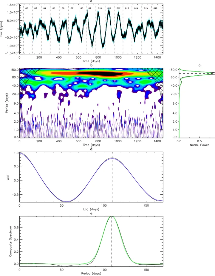
The methodology we apply here is similar to the one used in Garc´ıa et al. (2014a) adapted to study red giant stars. One of the differences is that only one type of data – KADACS corrected data – is used, with two different filters at 55 and 80 days. The first step of our methodology is computing a time-period anal-ysis based on a wavelets decomposition of the rebinned light curve to obtain the wavelet power spectrum (WPS). The WPS can be used to see if a modulation is due to a glitch or present during the whole data set. We then project this WPS on the pe-riod axis to form the global wavelets power spectrum (GWPS) which is similar to a Fourier spectrum but with a reduced reso-lution. The advantage of the GWPS is that it increases the power of the fundamental period of a signal and thus avoids mistak-ing an overtone for the true periodicity of the signal (Mathur et al. 2013). The GWPS is then described and least-squared min-imized using multiple Gaussian functions. The central period of the Gaussian function corresponding to the highest peak is then taken as the rotation period Prot,GWPS. The width at half-maximum of this function is taken as the uncertainty on this value. In the case of red giants, the solar-like oscillations can have periods of the order of a day and could be mistaken for ro-tation. To prevent this, we use the measured power excess and we exclude the range [νmax− 5∆ν ; νmax+ 5∆ν] from the search
for a rotation period. We have verified with stars of different νmax
and a wide range of magnitudes that this range is the minimum interval we need to remove to avoid any pollution of the rotation period measurements by the oscillation modes. This range is di-rectly interpolated in the GWPS prior to the fitting with Gaussian functions. Examples of the WPS and the GWPS can be seen in Fig. 2.
The second step of the methodology is calculating the autocorrelation function (ACF) of the light curve, following McQuillan et al. (2013b). The ACF is smoothed according to the most significant period present in its Lomb-Scargle peri-odogram. The smoothing is performed using a Gaussian function of width a tenth of the selected period. However, if this period is smaller than the one corresponding to the frequency νmax− 5∆ν,
that one is taken instead. The significant peaks in the smoothed ACF are then identified. The highest peak is taken as the rota-tion period Prot,ACF. The presence of a regular pattern due to the presence of several active regions on the star at different longi-tudes, as noted by McQuillan et al. (2013b), is also checked. If no significant peak is identified, the star is considered inactive (or observed with a very low inclination angle). An example of the ACF can be seen in Fig. 2.
3.2. Composite spectrum
The third method is a combination of the two previous ones. We create a new function, called the Composite Spectrum, that is ob-tained by multiplying the ACF and the GWPS together (Ceillier et al. 2016). This is done to boost the height of the peaks present in both curves and decrease the height of the peaks present in only one of the two. As the ACF and the GWPS are not sensitive to the same problems in the original light curve, this allows us to identify more easily periods intrinsic to the star.
To do so, we first fit the smoothed ACF with an exponentially decreasing function of the form
Fig. 2. Analysis of the light curve of KIC 2436732, filtered at 80 days. Panel a: original light curve (light blue) and rebinned light curve (black). Panel b: wavelet decomposition (WPS) of the rebinned light curve. Panel c: GWPS (black) and gaussian fit (green). Panel d: ACF of the rebinned light curve (black) and smoothed version of this ACF (blue). Panel e: composite spectrum of the rebinned light curve (black) and gaussian fit (green). For each method, a dashed line indicates the returned period.
where P is the period and A0 and A1 are the two parameters
to fit. We note that fexp(0) = 1 and fexp(∞) = 0. This fit is
then subtracted from the smoothed ACF. The normalized ACF is then rebinned into the periods of the GWPS to allow the proper multiplication of the two quantities.
The Composite Spectrum (CS) is then obtained by multiply-ing the normalized ACF by the normalized GWPS. This allows the Composite Spectra of all stars to have comparable amplitude. The CS has approximately the same resolution as the GWPS and is defined on the same periods. It allows a direct reading of the relevant periods present in the original light curve. As for the GWPS, the CS is fitted with multiple Gaussian functions. The central period of the function corresponding to the highest peak is taken as Prot,CS and the half-width at half-maximum of this
function is taken as the uncertainty on this value. An example of the CS can be seen in Fig. 2.
This methodology has been tested on a large sample of com-posite light curves in a hare-and-hounds exercise and has been found to be one of the best compromises between completeness and accuracy among all the available methodologies (Aigrain et al. 2015). In this work, we apply it to the light curves ob-tained with the 55 and 80 days filters, outputting six periods for each star: Prot,GWPS, Prot,ACF, and Prot,CS for each filter.
3.3. Automatic selection of probable detections
In the previous work detailed in Garc´ıa et al. (2014a), the rel-atively small size of the sample allowed us to perform a visual check of the results for each star. For the present work, the huge size of the sample prevents us from using the same, very time consuming, method. Moreover, only a small number of red giant stars are expected to show light curve modulations due to spots. We therefore need an automated way to extract from our initial sample a sub-sample containing only the potentially rotating red giants.
To do so, we introduce three values: HACF, HCS and GACF.
HACFis the height of the peak in the smoothed ACF that
corre-sponds to the rotation period Prot,ACF, as defined in McQuillan et al. (2013b). It is the mean of the difference between the value of the smoothed ACF at the top of the peak and the values of the smoothed ACF at the two neighbouring minima. HCS is defined
the same way but for the CS. Finally, GACF is the global
maxi-mum of the smoothed ACF after it first crossed 0, for the range of periods considered. While the reasons for which we consider the first two values are obvious, the use of GACFneeds to be
ex-plained. Its role is mostly to balance the fact that the way HACF
is computed does not give a precise idea of the degree of corre-lation between the light curve and itself with a lag of Prot,ACF,
as the maximum of the peak can be positive and small or even negative, with HACF still being high if the neighbouring minima
are very low. After testing several methods of balancing these effects, GACFis the most efficient and easiest to compute.
To validate the use of these three values and decide which threshold we should use for each of them, we calculated HACF,
HCS and GACF for the KADACS corrected light curves of the
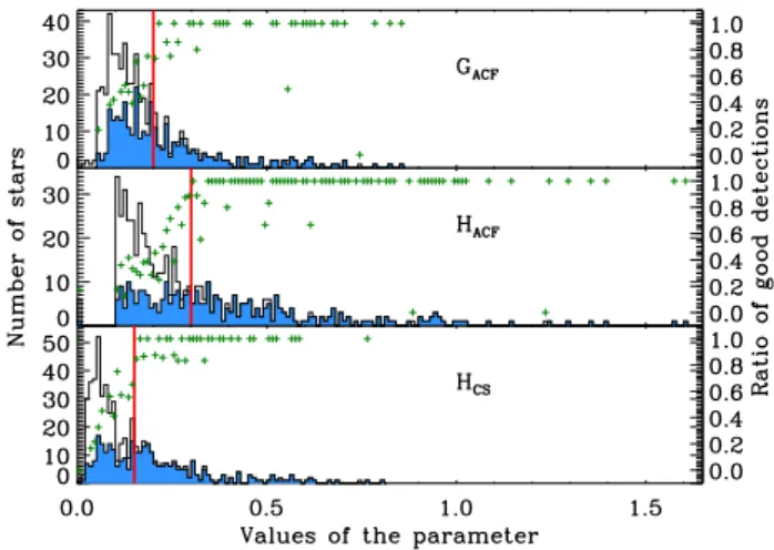
540 solar-like stars in Garc´ıa et al. (2014a). Fig 3 shows the his-tograms of these three values, both for the whole sample of 540 stars and for the 310 stars with detected surface rotation. We find that if we select all the stars with HACF ≥ 0.3, HCS ≥ 0.15 and
GACF ≥ 0.2, we recover 124 of the 310 stars showing rotation
(40%) and only 6 of the 230 stars showing no rotation (2.6%). The key point here is that the subsample thus obtained contains only 4.6% (6/130) stars without detected rotation. This selection
Fig. 3. Histograms of GACF, HACF, and HCS for the stars studied
by Garc´ıa et al. (2014a). Black lines: whole sample (540 stars). Blue: stars with detected surface rotation (310 stars). The green crosses represent the ratio of good detections for each bin and the red lines mark the threshold value used for each parameter.
method is then well suited to isolate a sample of stars with a high probability of detectable surface rotation.
Applying this selection method to our sample of 17,377 red giants, we isolate 925 stars for which the criterion (HACF ≥ 0.3,
HCS ≥ 0.15 and GACF ≥ 0.2) is fulfilled for at least one of the
two filters (55 or 80 days). For now on, we will only deal with this reduced sample. The remaining stars will be considered to have a low probability of detectable surface rotation.
3.4. Visual check of the sub-sample’s results
As the Kepler light curves can be sensitive to instrumental ef-fects, we then visually check the light curve, GWPS, ACF, and CS for each of the 925 stars and for both filters. If the period de-tected by one of these analyses is also visible in the light curve as stellar signal, this period is kept as the rotation period of the star. In contrast, when the signatures in the different methods are not clear enough or come from instrumental effects, no period is returned.
When it appears that the period detected seems to be a har-monic of the real rotation period, we apply a longer filter to the data and re-do the rotation period extraction process. This can happen when the first peak in the ACF is at a period below 100 days but the second and higher ones are at a period higher than 100 days. It can be due to spots or active regions appearing on opposite sides of the star and producing this characteristic pat-tern (see McQuillan et al. 2013a).
After this phase of visual inspection, only 531 stars out of the 925 of our sub-sample are kept. The light curves of all these stars demonstrate clear rotational modulations. For these 531 red giants, the final rotation period is taken from the fit of the cor-responding peak in the GWPS. The returned value Prot is the
period of the maximum of the gaussian function fitted while the uncertainty δProtis the half-width at half-maximum of this
func-tion. When possible, these values are taken from the GWPS of the 80 days-filtered light curve. Otherwise, the GWPS of the 55 days-filtered light curve is used.
Fig. 4. Distribution of stars showing rotational modulation in the Prot-∆ν space. Open grey dots correspond to the 151 stars discarded
according to the “crowding” criterion. Filled magenta dots are the 19 stars removed according to Tcritcriterion. Blue dots represent
stars for which a reliable rotation period has been derived (361 stars). The grey line indicates the critical period Tcritand the red
line marks a rotational velocity of 80% the critical one. The open square symbols indicate RGB stars with depressed dipolar modes following Stello et al. (2016b) while stars with normal dipolar modes are represented by a star symbol.
3.5. Discarding probable pollutions
In some cases, it is possible that the rotational modulation de-tected is not produced by the observed red giant. This can hap-pen for two reasons: the red giant is in fact part of a multiple system and the modulation is produced by an active companion star or there exists another active star that is close to the red giant on the sky and whose light is contaminating the red giant’s light curve, a chance alignment (Colman et al. 2017). In the first sce-nario, it is difficult to detect the presence of a companion without a detailed study of the star, including spectroscopic observations to check for multiple spectral lines or radial velocity variations.
In the second scenario, which is more likely to be the dom-inant one as MS stars are likely to be very faint relative to giants, it is possible to estimate the probability that the mask used to compute the red giant’s light cruve contains signal from other stars. The Kepler data products contain a parameter called crowding1, ranging from 0 to 1, that corresponds to the fraction of the flux from the target star. In other words, the closer to 1 this parameter is, the less polluted the light curve. We thus dis-card all the red giants among the 531 for which the crowding parameter is lower than 0.98, eliminating 151. Interestingly, the proportion of low-crowding stars is very high among the red gi-ants with rotation periods of less than 30 days, which shows that
1 The crowding values used here were the ones provided by the
MAST at https://archive.stsci.edu/kepler/ on April 2015.
most of these detections are due to pollution of the light curves. In contrast, the proportion of low-crowding stars is very low for red giants with rotation periods above 100 days, which tends to validate these detections.
3.6. Comparison with breakup rotation periods
Finally, we compare the rotation rate of stars with the critical period Tcrit under which a star would be torn apart by the
cen-trifugal force. This period can be calculated as follows:
Tcrit=
r 27π2R3
2GM , (2)
where R and M are the radius and the mass of the star and G is the gravitational constant. Using seismic scaling laws (see Kjeldsen & Bedding 1995), this expression can be simplified:
Tcrit= s 27π2R 3 2GM ∆ν ∆ν !−1 , (3)
where R , M and∆ν are the radius, the mass and the large
separation of the Sun and∆ν is the large separation of the star (see grey line in Fig. 4).
For each of the 531 stars, we calculate this critical period. If the measured period Protis lower than 1.25 Tcrit– corresponding
4) – we consider the measurement as doubtful. The modulation in the light curve could be due either to pollution of another star or to the presence of a companion in a binary system (causing modulation by the binary orbit rather than due to the rotation period of the giant star).
Prot and Tcrit are illustrated in Fig. 4 as a function of ∆ν,
which represents the mean density of the stars and provides some information on the evolutionary stage of the stars (red clump stars are located between 3 and 4.5 µHz). We clearly see that many of the stars with a rotation period smaller than the critical period were already discarded by the pollution criterion. Among the 380 stars with a crowding above 0.98 (i.e. passed the pollu-tion criterion), we find that nineteen stars are rotating faster than the Tcritcriterion (magenta dots in Fig. 4).
In some other cases, it is also possible that the derived value of ∆ν is incorrect, leading to a wrong value of Tcrit. However,
we can see in Fig 4 and Fig 5 that some, generally smaller, red giants with a rotation periods below thirty days are not discarded by this verification.
3.7. Comparison with known Kepler binaries
We have cross-checked our sample of 531 stars showing rota-tional modulation with the Villanova binary catalog (Kirk et al. 2016) containing all the known binaries in the Kepler main mis-sion. We found that only one star is a binary: KIC 5990753, with an orbital period of 7.2 days2.
In addition, we have also cross-checked our dataset with the list of Kepler compact binary systems around red giants stud-ied by (Colman et al. 2017). From a total of 168 stars analyzed in that paper, only 10 stars are in common with our 531 red gi-ants. Six of them are possible true compact binaries but only one, KIC 12003253, is retained in our final list of 361 “confirmed ro-tation” red giants. The other five were flagged as flag 1 or 2. The reported peak associated to the orbital modulation of the sec-ondary star in this system is 2 days and our rotation period for the red giant is 54 days. Therefore, we think the value reported in our paper is the true rotation period of the red giant. The other 4 star in common were reported as possible chance alignments or pollution in Colman’s paper. Three of these four stars are also flagged in our analysis (flag 1). The last one, KIC 7604896, is polluted by a signal with a period of 0.16 days as indicated in Colman et al. (2017), while our rotation period is 88.46 days. Therefore, we also think the value we reported is the rotation of the red giant.
3.8. Link between surface rotation and mode suppression The reduction in power of non-radial modes observed in red giants (Mosser et al. 2012, 2017; Garc´ıa et al. 2014c; Stello et al. 2016a) has been proposed to arise from magnetic suppres-sion (Fuller et al. 2015; Loi & Papaloizou 2017). The magnetic fields are thought to have been formed in the progenitor stars during the main sequence phase by a dynamo established due to the convection and rotation in the core regions (Stello et al. 2016b). If we assume that the surface rotation in the red gi-ant phase correlates with the core rotation during the main se-quence, we might expect that rapidly rotating red giants might have had faster main sequence core rotation rates and thus be more likely to have suppressed non-radial modes. To study this potential link, we cross matched the RGB stars investigated by Stello et al. (2016b) for mode suppression (i.e. stars with ∆ν
2 http://keplerebs.villanova.edu/overview/?k=5990753
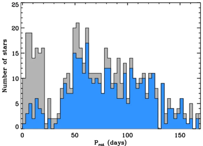
Fig. 5. Histograms of the rotation periods Prot for all the stars
showing rotational modulation (grey, 531 stars) and for stars for which a reliable rotation period has been derived (blue, 361 stars).
greater than 5 µHz to avoid including clump stars) with our RGB stars with∆ν above the same threshold and with reliable rotation measurements (131 stars). We found twelve stars that show sup-pression in our sample (blue filled dots surrounded by an open blue square in Fig. 4), and nine stars with normal oscillation mode power (blue filled dots surrounded by an open star sym-bol in Fig. 4). Of the eleven fast rotators (Prot < 30 days) in
that sample, six show suppressed modes and five show a normal oscillation pattern. For comparison, of the ten slow rotators in the sample (Prot > 30 days), there are six with depressed dipole
modes, and four normal oscillators. We therefore see no obvious correlation between the two phenomena (rapid surface rotation and suppressed dipole modes) in our sample. Additional anal-ysis should be done when a larger sample is available to infer stronger conclusions.
4. Results and discussion
We initially detected 531 stars showing signature of rotational modulation. From this set we remove 151 stars due to the crowd-ing factor. We also discard 19 additional stars whose rotation rate is close to, or faster than, the critical break-up period. Thus, we keep a sample of 361 stars with confirmed surface rotation pe-riods. These results are summarised in Table 1 and the distribu-tion of the derived Protcan be seen in Fig 5. It is clear that while
short periods are more likely to be detectable, they are also more likely to be a signal from a companion or contaminant. In con-trast, longer periods are more likely to be from the red giant, but we suspect that the fall off at longer periods is a selection effect, as long period, low amplitude signals are the most difficult to detect. In these tables, we also give the values of the global pa-rameters of the p modes (∆ν and νmax) with the mass and surface
gravity computed from the seismic scaling relations.
Now that the sample of stars is defined we can compare our results with spectroscopic measurements and study the distribu-tion of the active red giants that we detected to better understand the underlying scenarios explaining this high activity and rota-tion.
Table 1. Stars with validated rotation periods.
KIC νmax[µHz] ∆ν [µHz] Teff[K] log g [dex] M [M ] Prot[days] crowding Tcrit[days] vsini[km/s]
1161618 34.25 ± 1.88 4.09 ± 0.14 4855 ± 161 1.29 ± 0.16 2.45 ± 0.03 158.34 ± 7.90 0.990 7.26 0.00 ± 0.00 1162746 27.58 ± 1.81 3.64 ± 0.13 5141 ± 308 1.17 ± 0.18 2.37 ± 0.04 46.74 ± 4.72 1.000 8.16 0.00 ± 0.00 1871631 29.29 ± 2.15 3.71 ± 0.11 4823 ± 108 1.18 ± 0.17 2.38 ± 0.03 44.54 ± 3.08 0.990 8.01 0.00 ± 0.00 2018667 30.73 ± 1.80 3.83 ± 0.14 4773 ± 123 1.19 ± 0.15 2.40 ± 0.03 65.67 ± 3.52 0.990 7.75 0.00 ± 0.00 2019396 37.98 ± 1.89 4.16 ± 0.13 4790 ± 100 1.62 ± 0.18 2.49 ± 0.02 63.86 ± 8.70 0.990 7.14 0.00 ± 0.00 2156178 29.08 ± 1.87 3.93 ± 1.91 5099 ± 225 1.00 ± 0.98 2.39 ± 0.03 40.98 ± 3.18 1.000 7.56 0.00 ± 0.00 2305930 28.27 ± 1.78 3.97 ± 0.14 4924 ± 173 0.84 ± 0.11 2.37 ± 0.03 33.75 ± 2.52 0.990 7.48 13.09 ± 0.88 2436732 30.34 ± 1.76 3.70 ± 0.11 4719 ± 147 1.29 ± 0.16 2.39 ± 0.03 109.63 ± 5.17 0.980 8.03 0.00 ± 0.00 2447529 106.95 ± 4.87 8.38 ± 0.18 5186 ± 247 2.47 ± 0.26 2.96 ± 0.03 98.83 ± 5.49 0.990 3.54 0.00 ± 0.00 2716214 30.26 ± 1.95 3.91 ± 0.12 5120 ± 279 1.16 ± 0.17 2.41 ± 0.03 41.31 ± 2.07 0.990 7.60 0.00 ± 0.00 2845408 74.76 ± 3.95 6.38 ± 0.12 5058 ± 185 2.42 ± 0.26 2.80 ± 0.03 142.71 ± 14.66 0.990 4.66 0.00 ± 0.00 2845610 90.10 ± 5.20 6.97 ± 0.14 5095 ± 151 3.00 ± 0.34 2.88 ± 0.03 79.72 ± 8.51 1.000 4.26 0.00 ± 0.00 2854994 133.16 ± 10.78 10.26 ± 0.21 5003 ± 117 2.01 ± 0.30 3.05 ± 0.04 132.27 ± 6.54 1.000 2.89 0.00 ± 0.00 2856412 35.67 ± 2.05 4.23 ± 0.58 4904 ± 222 1.30 ± 0.39 2.47 ± 0.03 9.77 ± 0.52 0.990 7.02 0.00 ± 0.00 2860936 102.01 ± 5.63 7.59 ± 0.84 5062 ± 144 3.07 ± 0.75 2.93 ± 0.03 114.32 ± 5.55 1.000 3.91 0.00 ± 0.00 2988655 30.63 ± 1.70 3.87 ± 0.61 5158 ± 313 1.27 ± 0.43 2.42 ± 0.03 71.85 ± 6.93 0.990 7.67 0.00 ± 0.00 3102990 29.77 ± 1.86 3.79 ± 0.56 4835 ± 177 1.15 ± 0.36 2.39 ± 0.03 85.44 ± 7.84 1.000 7.84 0.00 ± 0.00 3216467 31.47 ± 1.96 3.83 ± 0.12 4623 ± 154 1.21 ± 0.16 2.40 ± 0.03 151.87 ± 8.36 0.990 7.75 0.00 ± 0.00 3220837 132.56 ± 20.10 13.21 ± 0.31 5294 ± 260 0.79 ± 0.21 3.06 ± 0.07 79.73 ± 7.54 0.990 2.25 0.00 ± 0.00 3240280 29.19 ± 1.71 3.78 ± 1.71 4810 ± 121 1.08 ± 0.99 2.38 ± 0.03 103.83 ± 5.30 0.990 7.86 0.00 ± 0.00 3324186 32.44 ± 2.20 3.91 ± 0.09 4724 ± 110 1.26 ± 0.16 2.42 ± 0.03 51.87 ± 4.32 0.980 7.60 0.00 ± 0.00 3432732 80.48 ± 3.81 6.45 ± 0.13 5015 ± 150 2.85 ± 0.28 2.83 ± 0.02 121.75 ± 5.62 1.000 4.60 0.00 ± 0.00 3437031 63.45 ± 2.74 5.60 ± 0.18 5059 ± 214 2.49 ± 0.28 2.73 ± 0.02 138.77 ± 7.22 0.990 5.30 0.00 ± 0.00 3439466 29.33 ± 1.65 3.91 ± 0.11 4991 ± 235 1.01 ± 0.13 2.39 ± 0.03 46.75 ± 4.41 0.990 7.60 0.00 ± 0.00 3448282 30.45 ± 1.54 3.59 ± 0.09 4891 ± 241 1.55 ± 0.18 2.40 ± 0.03 55.98 ± 4.69 0.990 8.27 0.00 ± 0.00 3526625 34.35 ± 2.51 4.18 ± 0.15 4883 ± 184 1.21 ± 0.18 2.45 ± 0.04 125.11 ± 5.95 1.000 7.11 0.00 ± 0.00 3532985 94.84 ± 10.80 7.92 ± 0.27 4752 ± 122 1.89 ± 0.40 2.89 ± 0.05 6.03 ± 0.29 0.990 3.75 0.00 ± 0.00 3557606 100.96 ± 6.24 8.09 ± 0.24 5044 ± 118 2.29 ± 0.29 2.93 ± 0.03 26.34 ± 2.99 0.990 3.67 0.00 ± 0.00 3642135 51.25 ± 2.53 4.96 ± 0.15 5060 ± 175 2.13 ± 0.24 2.64 ± 0.02 144.72 ± 7.10 1.000 5.99 0.00 ± 0.00 3750783 110.02 ± 4.91 8.68 ± 0.20 5249 ± 300 2.38 ± 0.27 2.97 ± 0.03 6.79 ± 0.45 0.990 3.42 0.00 ± 0.00 3758731 74.83 ± 5.98 6.28 ± 0.18 5119 ± 248 2.63 ± 0.42 2.80 ± 0.04 115.12 ± 3.69 1.000 4.73 0.00 ± 0.00 3937217 30.06 ± 1.94 3.76 ± 0.11 4887 ± 185 1.24 ± 0.17 2.40 ± 0.03 54.08 ± 4.43 1.000 7.90 9.08 ± 1.42 3956210 29.67 ± 3.21 3.85 ± 0.50 5015 ± 214 1.13 ± 0.37 2.40 ± 0.05 54.83 ± 4.94 0.990 7.71 0.00 ± 0.00 4041075 32.20 ± 2.00 3.78 ± 0.13 4290 ± 156 1.23 ± 0.17 2.40 ± 0.03 111.25 ± 5.14 1.000 7.86 0.00 ± 0.00 ... ... ... ... ... ... ... ... ...
Notes: The crowding value represents the amount of the integrated flux belonging to the targeted star. Hence, it is equal to one when only the targeted star is in the aperture.
4.1. Comparison with v sin(i) measurements
The most common alternate method for studying stellar sur-face rotation is measuring the rotational line broadening v sin(i) through spectroscopic observations. Such measurements are completely independent from our analysis and allow us to ver-ify whether the rotation periods we extract are compatible with other observations. Moreover, we can estimate the radii of the stars of our sample from their seismic global parameters – νmax
and∆ν – and their effective temperatures Teff– taken from Huber
et al. (2014). This then allows the estimation of the inclination angle i, a parameter that is otherwise difficult to constrain ex-cept from a detailed seismic analysis or from a modeling of the transits for multiple systems.
Fig. 6 presents the comparison between the Prot from this
work with the maximum period possible for the v sin(i) derived by Tayar et al. (2015) from APOGEE spectra. It shows that the periods we derive are fully compatible with the spectroscopic measurements. Moreover, the distribution of sin(i) is relatively compatible with a uniform random distribution of the angles i. This suggests that our sample of rotating red giants is not biased towards particular inclination angles.
4.2. Binarity
While isolated giants are not generally expected to have measur-able spots, the same is not true for giants in close, tidally interact-ing binary systems (e.g. Gaulme et al. 2014; Beck et al. 2017). Similar to the W Ursa Majoris stars, tidal interactions tend to enhance surface activity and increase rotation rates. While not all of the stars in our sample have multiple epochs of spec-troscopic observations, we searched the 116 stars in our vali-dated sample with multiple APOGEE spectra for radial velocity variability greater than 1 km s−1. That threshold is larger than
both the detection limit for this instrument (0.5 km/s; Deshpande et al. 2013) and the expected radial velocity jitter for red giants (a surface gravity dependent quantity which can be as high as 0.5 km/s at a log(g) of 1; Hekker et al. 2008). We find sig-nificant radial velocity variability (greater than 1 km/s) in six stars (5.2% of the searchable sample; KIC 5382824, 5439339, 6032639, 6933666, 7531136, and 12314910); two others (KIC 7661609 and 9240941) have suggestive variations (greater than 0.5 km/s, less than 1 km/s). Although very unlikely, it could be possible that the periods measured for these stars are actually the rotation periods of their lower mass companions. However, we suspect that in most cases the secondary is much smaller and therefore unlikely to substantially contribute to the variability of the blended source. Moreover, the rotation rates found for these
Table 2. Stars showing rotational modulation in their light curve but probably due to a pollution of a nearby star.
KIC νmax[µHz] ∆ν [µHz] Teff[K] log g [dex] M [M ] Prot[days] crowding Tcrit Flag
1164356 27.80 ± 1.80 3.33 ± 0.09 5225 ± 169 2.38 ± 0.03 1.76 ± 0.23 15.21 ± 1.18 0.770 8.92 1 1870433 229.14 ± 25.83 16.14 ± 0.52 5099 ± 191 3.29 ± 0.05 1.72 ± 0.36 90.81 ± 4.40 0.970 1.84 1 2157901 28.89 ± 2.70 3.93 ± 0.11 4998 ± 277 2.38 ± 0.05 0.95 ± 0.18 43.92 ± 3.37 0.650 7.56 1 2305407 139.13 ± 20.11 13.07 ± 0.30 5017 ± 127 3.07 ± 0.07 0.87 ± 0.22 92.15 ± 4.31 0.980 2.27 1 2436944 30.40 ± 1.74 3.75 ± 0.11 4835 ± 192 2.40 ± 0.03 1.27 ± 0.16 135.06 ± 5.78 0.860 7.92 1 2437653 74.10 ± 3.40 7.03 ± 0.21 4386 ± 130 2.76 ± 0.02 1.29 ± 0.14 10.97 ± 1.03 0.880 4.22 1 2437987 30.32 ± 1.80 3.68 ± 0.10 4708 ± 135 2.39 ± 0.03 1.31 ± 0.16 113.56 ± 5.68 0.880 8.07 1 2438051 30.89 ± 1.64 3.66 ± 0.11 4724 ± 139 2.40 ± 0.03 1.42 ± 0.16 80.83 ± 7.30 0.970 8.12 1 2570214 25.44 ± 1.65 3.65 ± 0.08 4735 ± 148 2.32 ± 0.03 0.81 ± 0.10 69.40 ± 5.22 0.970 8.14 1 2570518 46.10 ± 2.70 4.94 ± 0.15 4399 ± 130 2.56 ± 0.03 1.28 ± 0.16 10.11 ± 0.73 0.870 6.01 1 2719113 32.58 ± 1.80 3.96 ± 0.12 4695 ± 122 2.42 ± 0.03 1.21 ± 0.14 94.80 ± 9.70 0.970 7.50 1 2720444 32.03 ± 2.72 4.08 ± 0.10 5013 ± 233 2.43 ± 0.04 1.12 ± 0.19 67.04 ± 7.32 0.980 7.28 1 2833697 30.95 ± 2.14 4.11 ± 0.13 5117 ± 126 2.42 ± 0.03 1.01 ± 0.14 42.13 ± 2.85 0.950 7.23 1 3234655 41.57 ± 2.36 4.52 ± 0.13 5233 ± 377 2.55 ± 0.03 1.74 ± 0.25 128.09 ± 5.07 0.980 6.57 1 3240573 31.80 ± 2.28 3.89 ± 0.12 4752 ± 166 2.41 ± 0.03 1.23 ± 0.18 68.51 ± 3.52 0.970 7.64 1 ... ... ... ... ... ... ... ... ...
Notes: The value of the flag is equal to 1 if the star has been discarded because of a low crowding value and 2 if it has been discarded because the ratio Prot/Tcritis too small (see Section 3 for details).
Fig. 6. Top: comparison between the Prot from this work and
the maximum period Pspeccompatible with vsin(i) measured by
Tayar et al. (2015). The different lines indicate where a star is ex-pected to fall for a given inclination angle i. Bottom: Distribution of the sin(i) for the rotation sample. The dotted line corresponds to the distribution expected for a random distribution of inclina-tions.
giants are very similar to those found for the rest of the sample, which suggests that they are due to spots on the primary.
4.3. Causes of Rapid Rotation in Single Stars
Because the stars in our sample have measured masses, we want to compare the distribution of active stars we measure to previ-ous measurements of rapid rotation as well as population synthe-sis models to determine whether our rapidly rotating single stars are massive stars born with rapid rotation or stars that must have gained angular momentum through an interaction. Spectroscopic surveys indicate that about 2 percent of red giants are rotating rapidly (vsini> 10 km s−1, Carlberg et al. 2011). While it is
dif-ficult to directly compare our period detection fraction to these spectroscopic rotation predictions because of unknown factors like the interplay between rotation and magnetic excitation, we suspect that given observed correlations between rotation and activity (e.g. Noyes et al. 1984; Mamajek & Hillenbrand 2008), the fraction of stars with detected photometric periods should be similar to the fraction of rapidly rotating stars. Indeed, we find that we detect periodic modulations in 2.08% (361/17,377 ) of our sample, which is consistent with the fraction of spectro-scopically measured rapid rotators. We therefore assume for the following analysis that the fraction of active stars we measure is related to the fraction of rapid rotators measured by spectro-scopic methods. We remind the reader that our actual sample is the fraction of stars active enough to measure rotation periods and that we have no information on the distribution of the rota-tion periods in inactive stars.
Population synthesis models indicate that one to two per-cent of stars should be rapidly rotating from reper-cent interac-tions or mergers with a companion star (Carlberg et al. 2011). Additionally, angular momentum conservation in intermediate mass stars predicts that an additional few percent of field giants should be rotating rapidly because they have not yet spun down. Because our stars have measured masses and surface gravities, we focus in on two regions of parameter space (see Figure 7).
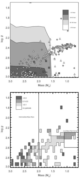
The first region is the low-mass red clump. These are stars that rotated slowly on the main sequence and therefore (see Figure 7, top) they can not have rotation detected at the peri-ods we search on the giant branch unless they gain angular mo-mentum from an interaction with another object. It has recently
Fig. 7. Top: Background colors indicated the prediction for the minimum rotation period expected for single stars from models in Tayar et al. (2015) with <30 days in dark grey, 30-90 days in medium grey, 90-180 days in light grey, and >180 days in white. For comparison, we overplot the measured rotation peri-ods for stars in our sample using the same period bins as dark grey squares, medium grey diamonds, and light grey triangles. Bottom: Fraction of stars with detected rotation periods in bins of mass and surface gravity. Dark grey indicates bins where > 30% of the stars had detected rotation, medium grey indicates bins with 10 − 30% detections, light grey indicates bins where fewer than 10% of stars had detected rotation periods, and white indicates bins with either no stars or no detected rotation periods. We have also indicated the regions we define as ‘intermediate mass’ and ‘low-mass red clump’.
been suggested that more than 7% of low-mass red clump stars are spun up as the result of an interaction (Tayar et al. 2015). We detect rotation in 88 (15.3%)of the 575 Kepler giants with masses below 1.1M and surface gravities between 2.3 and 2.6
dex, which is twice this previous measurement. We therefore suggest that a large fraction of red giants have undergone an interaction on the giant branch that spins up their surface and that the unexpectedly low number of fast rotators to an overes-timation of the stellar merger rates. Additionally, although it is out of the scope of this paper, it would be very interesting to study these red giants in more detail and especially to measure their surface abundances and check if there is an enrichment in certain elements due to this interaction.
The second region we analyzed contains the intermediate mass stars. Observations indicate that intermediate mass stars (M > 2.0 M ) have a wide range of rotation rates on the main
sequence (Zorec & Royer 2012). Assuming solid body rotation and solar-like angular momentum loss, more than fifty percent of intermediate mass stars should still have rotation velocities above 10 km/s on the giant branch. In contrast with such pre-dictions, we find a smaller rate of rotating stars above two solar masses (94 out of 4881 Kepler giants in this mass range; 1.92%), and find that rotation is detected only in the smallest stars in this mass range (see Figure 7, bottom). This suggests that intermedi-ate mass stars are either losing more angular momentum than a standard Kawaler wind loss law would predict (Kawaler 1988), or they are undergoing a substantial amount of radial di fferen-tial rotation. Seismic measurements of the core rotation of a few such stars indicate that radial differential rotation is occurring (e.g. Beck et al. 2012; Deheuvels et al. 2015), but more work should be done to characterize the extent of the differential ro-tation and the extent to which additional loss is required. We therefore suggest that the low fraction of active stars in our sam-ple is due to an incorrect estimation of the fraction of rapidly rotating intermediate mass stars.
5. Conclusions
We study a sample of 17,377 red giants with measured solar-like oscillations from the Kepler observations. We use various techniques to detect the active stars in this sample and mea-sure their surface rotation rates from modulations of their light curves. After carefully taking into account possible pollutants, we extract a sub-sample of 361 red giants with accurate surface rotation periods.
These red giants are peculiar in the sense that they show high activity and rapid rotation. While we assume in this analysis that activity and rotation are correlated, we reemphasize that we do not measure the distribution of rotation periods in inactive stars. However we suspect that most of the inactive stars are rotating slowly, due to the expansion of their outer layers and the extrac-tion of angular momentum through magnetized winds during the main sequence. We therefore assert that the majority of the ac-tive, rapidly rotating stars in our sample must have undergone an event that led to an acceleration of their surface rotation.
Our detection rate of 2.08% is indeed in very good agree-ment with binary interactions predictions from Carlberg et al. (2011). Moreover, this rate becomes equal to 15.3% if we con-sider only the low-mass red clump stars our our sample, which shows that red giants that have gone through the whole red giant branch have a higher probability of having undergone an inter-action with a companion, star or planet, as suggested by Tayar et al. (2015).
However, when we consider only more massive stars that did not lose angular momentum on the main sequence and should therefore be rotating rapidly, we do not see the enhanced rate of detections that we would have expected. This suggests that the discrepancy between the predicted and measured rates of rapid rotation in the field comes from the overestimation of the sur-face rotation rates of intermediate mass red giants. It indicates a complexity to the angular momentum transport and loss in these stars that is not currently taken into account and we suggest that more work should be done to understand how these stars differ from solar-type dwarfs.
This work opens the path to a large number of studies about red giant stars. It can help to better understand the links between activity and rotation for these objects as it offers a sample of active and rapidly rotating red giants to the stellar community. In particular, it would be interesting to see if any evidence can be obtained that the red clump stars from our sub-sample have indeed undergone an interaction with a companion.
Acknowledgements. The authors wish to thank the entire Kepler team, without whom these results would not be possible. Funding for this Discovery mission is provided by NASA’s Science Mission Directorate. The authors also wish to thank R.-M. Ouazzani for very fruitful discussions on this work. The authors acknowl-edges the KITP staff of UCSB for their hospitality during the research program Galactic Archaeology and Precision Stellar Astrophysics. MHP and JT acknowl-edge support from NSF grant AST-1411685. TC, DS, and RAG received funding from the CNES GOLF and PLATO grants at CEA. RAG and PGB acknowledge the ANR (Agence Nationale de la Recherche, France) program IDEE (ANR-12-BS05-0008) “Interaction Des ´Etoiles et des Exoplan`etes”. SM acknowledges support from NASA grants NNX12AE17G and NNX15AF13G and NSF grant AST-1411685. The research leading to these results has received funding from the European Communitys Seventh Framework Programme ([FP7/2007-2013]) under grant agreement no. 269194 (IRSES/ASK).
References
Aigrain, S., Llama, J., Ceillier, T., et al. 2015, MNRAS, 450, 3211 Barnes, S. A. 2003, ApJ, 586, 464
Barnes, S. A., Weingrill, J., Fritzewski, D., Strassmeier, K. G., & Platais, I. 2016, ApJ, 823, 16
Beck, P. G., Kallinger, T., Pavlovski, K., et al. 2017, A&A (submitted) Beck, P. G., Montalban, J., Kallinger, T., et al. 2012, Nature, 481, 55
Brown, T. M., Gilliland, R. L., Noyes, R. W., & Ramsey, L. W. 1991, ApJ, 368, 599
Cantiello, M., Mankovich, C., Bildsten, L., Christensen-Dalsgaard, J., & Paxton, B. 2014, ApJ, 788, 93
Carlberg, J. K., Majewski, S. R., & Arras, P. 2009, ApJ, 700, 832 Carlberg, J. K., Majewski, S. R., Patterson, R. J., et al. 2011, ApJ, 732, 39 Carlberg, J. K., Smith, V. V., Cunha, K., & Carpenter, K. G. 2016, ApJ, 818, 25 Carlberg, J. K. J. K., Majewski, S. R. S. R., Patterson, R. J. R. J., et al. 2011, The
Astrophysical Journal, 732, 39
Ceillier, T., Eggenberger, P., Garc´ıa, R. A., & Mathis, S. 2013, A&A, 555, A54 Ceillier, T., van Saders, J., Garc´ıa, R. A., et al. 2016, MNRAS, 456, 119 Colman, I. L., Huber, D., Bedding, T. R., et al. 2017, ArXiv e-prints de Medeiros, J. R., Da Rocha, C., & Mayor, M. 1996, A&A, 314, 499 Deheuvels, S., Ballot, J., Beck, P. G., et al. 2015, A&A, 580, A96
Deshpande, R., Blake, C. H., Bender, C. F., et al. 2013, The Astronomical Journal, 146, 156
do Nascimento, J.-D., da Costa, J. S., & Castro, M. 2012, A&A, 548, L1 Duchˆene, G. & Kraus, A. 2013, ARA&A, 51, 269
Durney, B. R. & Latour, J. 1978, Geophysical and Astrophysical Fluid Dynamics, 9, 241
Fekel, F. C. & Balachandran, S. 1993, ApJ, 403, 708
Fr¨ohlich, H.-E., Frasca, A., Catanzaro, G., et al. 2012, A&A, 543, A146 Fuller, J., Cantiello, M., Stello, D., Garcia, R. A., & Bildsten, L. 2015, Science,
350, 423
Garc´ıa, R. A., Ceillier, T., Mathur, S., & Salabert, D. 2013, in Astronomical Society of the Pacific Conference Series, Vol. 479, Astronomical Society of the Pacific Conference Series, ed. H. Shibahashi & A. E. Lynas-Gray, 129 Garc´ıa, R. A., Ceillier, T., Salabert, D., et al. 2014a, A&A, 572, A34 Garc´ıa, R. A., Hekker, S., Stello, D., et al. 2011, MNRAS, 414, L6 Garc´ıa, R. A., Mathur, S., Pires, S., et al. 2014b, A&A, 568, A10
Garc´ıa, R. A., P´erez Hern´andez, F., Benomar, O., et al. 2014c, A&A, 563, A84
Garc´ıa, R. A., R´egulo, C., Samadi, R., et al. 2009, A&A, 506, 41
Gaulme, P., Jackiewicz, J., Appourchaux, T., & Mosser, B. 2014, ApJ, 785, 5 Hekker, S., Gilliland, R. L., Elsworth, Y., et al. 2011, MNRAS, 414, 2594 Hekker, S., Snellen, I. A. G., Aerts, C., et al. 2008, Astronomy & Astrophysics,
480, 215
Huber, D., Bedding, T. R., Stello, D., et al. 2010, ApJ, 723, 1607 Huber, D., Silva Aguirre, V., Matthews, J. M., et al. 2014, ApJS, 211, 2 Kawaler, S. D. 1988, ApJ, 333, 236
Kirk, B., Conroy, K., Prˇsa, A., et al. 2016, AJ, 151, 68 Kjeldsen, H. & Bedding, T. R. 1995, A&A, 293, 87
Lanza, A. F., Das Chagas, M. L., & De Medeiros, J. R. 2014, A&A, 564, A50 Leiner, E., Mathieu, R. D., Stello, D., Vanderburg, A., & Sandquist, E. 2016,
ApJ, 832, L13
Loi, S. T. & Papaloizou, J. C. B. 2017, MNRAS, 467, 3212 Mamajek, E. E. & Hillenbrand, L. A. 2008, ApJ, 687, 1264
Martig, M., Fouesneau, M., Rix, H.-W., et al. 2016, MNRAS, 456, 3655 Martig, M., Rix, H.-W., Silva Aguirre, V., et al. 2015, MNRAS, 451, 2230 Massarotti, A., Latham, D. W., Stefanik, R. P., & Fogel, J. 2008, AJ, 135, 209 Mathur, S., Bruntt, H., Catala, C., et al. 2013, A&A, 549, A12
Mathur, S., Garc´ıa, R. A., Catala, C., et al. 2010a, A&A, 518, A53 Mathur, S., Garc´ıa, R. A., Huber, D., et al. 2016, ApJ, 827, 50 Mathur, S., Garc´ıa, R. A., R´egulo, C., et al. 2010b, A&A, 511, A46 McQuillan, A., Aigrain, S., & Mazeh, T. 2013a, MNRAS, 432, 1203 McQuillan, A., Mazeh, T., & Aigrain, S. 2013b, ApJ, 775, L11 McQuillan, A., Mazeh, T., & Aigrain, S. 2014, ApJS, 211, 24 Mosser, B., Belkacem, K., Pinc¸on, C., et al. 2017, A&A, 598, A62 Mosser, B., Elsworth, Y., Hekker, S., et al. 2012, A&A, 537, A30 Mosser, B., Michel, E., Appourchaux, T., et al. 2009, A&A, 506, 33 Ness, M., Hogg, D. W., Rix, H.-W., et al. 2016, ApJ, 823, 114
Nielsen, M. B., Gizon, L., Schunker, H., & Karoff, C. 2013, A&A, 557, L10 Noyes, R. W., Hartmann, L. W., Baliunas, S. L., Duncan, D. K., & Vaughan,
A. H. 1984, ApJ, 279, 763
Piotto, G., De Angeli, F., King, I. R., et al. 2004, ApJ, 604, L109 Pires, S., Mathur, S., Garc´ıa, R. A., et al. 2015, A&A, 574, A18 Privitera, G., Meynet, G., Eggenberger, P., et al. 2016, A&A, 593, A128 Raghavan, D., McAlister, H. A., Henry, T. J., et al. 2010, ApJS, 190, 1 Reimers, D. 1975, Circumstellar envelopes and mass loss of red giant stars, ed.
B. Baschek, W. H. Kegel, & G. Traving, 229–256 Schatzman, E. 1962, Annales d’Astrophysique, 25, 18 Skumanich, A. 1972, ApJ, 171, 565
Stello, D., Cantiello, M., Fuller, J., Garcia, R. A., & Huber, D. 2016a, PASA, 33, e011
Stello, D., Cantiello, M., Fuller, J., et al. 2016b, Nature, 529, 364 Stello, D., Huber, D., Bedding, T. R., et al. 2013, ApJ, 765, L41
Tayar, J., Ceillier, T., Garc´ıa-Hern´andez, D. A., et al. 2015, The Astrophysical Journal, 807, 82
Tayar, J. & Pinsonneault, M. H. 2013, ApJ, 775, L1
Thompson, S. E., Christiansen, J. L., Jenkins, J. M., et al. 2013, Kepler Data Release 21 Notes (KSCI-19061-001), Kepler mission
Weber, E. J. & Davis, Jr., L. 1967, ApJ, 148, 217