Brightest cluster galaxies in cosmological simulations with adaptive mesh
refinement: successes and failures
Davide Martizzi,
1‹Jimmy,
2Romain Teyssier
3and Ben Moore
31Department of Astronomy, University of California, Berkeley, CA 94720-3411, USA
2George P. and Cynthia W. Mitchell Institute for Fundamental Physics and Astronomy, Department of Physics and Astronomy, Texas A&M University, College Station, TX 77843, USA
3Institute for Computational Science, University of Zurich, CH-8057 Z¨urich, Switzerland
Accepted 2014 June 19. Received 2014 June 9; in original form 2014 May 2
A B S T R A C T
A large sample of cosmological hydrodynamical zoom-in simulations with adaptive mesh refinement is analysed to study the properties of simulated brightest cluster galaxies (BCGs). Following the formation and evolution of BCGs requires modelling an entire galaxy cluster, because the BCG properties are largely influenced by the state of the gas in the cluster and by interactions and mergers with satellites. BCG evolution is also deeply influenced by the presence of gas heating sources such as Active Galactic Nuclei (AGN) that prevent catastrophic cooling of large amounts of gas. We show that AGN feedback is one of the most important mechanisms in shaping the properties of BCGs at low redshift by analysing our statistical sample of simulations with and without AGN feedback. When AGN feedback is included BCG masses, sizes, star formation rates and kinematic properties are closer to those of the observed systems. Some small discrepancies are observed only for the most massive BCGs and in the fraction of star-forming BCGs, effects that might be due to physical processes that are not included in our model.
Key words: black hole physics – methods: numerical – galaxies: clusters: general – galaxies:
formation – cosmology: theory – large-scale structure of Universe.
1 I N T R O D U C T I O N
Brightest cluster galaxies (BCGs) are the most luminous and mas-sive galaxies in the Universe. They typically sit at (or close to) the centre of the most massive gravitationally bound structures, galaxy clusters. BCGs are one of the best examples of hierarchical galaxy formation and evolution. Since they sit at the bottom of deep clus-ter potential wells, they are exposed to a large number of events that modify their properties. Such processes include fast gas infall fuelling star formation during their early stage of evolution and dynamical interactions with satellite galaxies which fall into the cluster and eventually merge with the BCGs. On the other hand, the interaction of the satellite galaxies with their environment (e.g. other galaxies and the intracluster medium, ICM) determines the properties of the objects that merge with the BCGs, therefore in-fluence the post-merging properties of the BCGs themselves. The stellar material stripped from the satellite galaxies during their inter-action with the central potential ends up constituting the so-called intracluster light (ICL), i.e. an extended stellar halo surrounding the BCG and characterized by a rich variety of substructure (Gonza-lez, Zabludoff & Zaritsky2005; Gonz´alez, Audit & Huynh2007;
⋆ E-mail: [email protected]
Rudick et al.2010). Metal enrichment and physical state of the ICM at low redshift determine whether the central region of clusters and BCGs will be characterized by cooling flows that feed star forma-tion, i.e. the star formation rate (SFR) of the central galaxy. BCGs also host the most massive black holes in the Universe which can have masses up to a few 109
M⊙ (McConnell & Ma2013) and can influence the ICM state during their active galactic nuclei (AGN) phases (Fabian2012).
Given these considerations, it is appropriate to say that theoret-ical modelling of BCGs represents one of the most challenging problems in galaxy formation and evolution. Modelling BCGs re-quires also detailed modelling of the cluster environment and of the satellite galaxies. Ideal tools to study this problem are cosmological hydrodynamical simulations which try to model most of the rele-vant processes in galaxy formation. The problem of BCG formation has been already studied in detail in this context, e.g. by Ragone-Figueroa et al. (2013), and many results have been published on the properties of galaxy groups and clusters from the OWLs collab-oration (e.g. McCarthy et al.2011) and other groups (e.g. Sijacki et al.2007). These studies have all been performed by analysing smoothed particle hydrodynamics (SPH) simulations. Recently, we published the analysis of a series of high-resolution cosmologi-cal hydrodynamicosmologi-cal zoom-in simulations of a galaxy cluster and its BCG (Martizzi, Teyssier & Moore2012a) performed with the
adaptive mesh refinement (AMR) codeRAMSES(Teyssier2002). The
novelty of the analysis of Martizzi et al. (2012a) was that the BCG formation problem was addressed for the first time using an AMR code which included prescriptions for AGN feedback. In agree-ment with the result of other groups, we showed that realistic BCG properties could be obtained only if AGN feedback (or an equiv-alent source of heating) was included in the calculation to avoid catastrophic cooling of gas in the cluster core. Despite the excellent resolution of those calculations, the limit of the results shown in Martizzi et al. (2012a) is that they are relative to one halo only.
Studying the properties of BCGs provides a unique opportunity to test galaxy formation physics in AMR simulations. For this reason, we performed a study complementary to that of Martizzi et al. (2012a). In this paper, we analyse the BCGs in a large sample of cosmological hydrodynamical AMR zoom-in simulations (already presented in Martizzi et al.2014) at redshift z = 0. The goal of
this work is to study a statistical sample of simulated BCG and place constraint on the validity of the adopted galaxy formation prescriptions.
The paper is organized as follows. Section 1 is dedicated to de-scribing the methods and the simulations. Section 2 shows a detailed comparison of the simulated BCG properties to observational data. The final section is a summary of the results and contains the main conclusions drawn from the analysis.
2 N U M E R I C A L S I M U L AT I O N S
We consider a set of 102 cosmological re-simulations performed with theRAMSEScode (Teyssier2002). These simulations are part of a
larger set recently used in Martizzi et al. (2014) to study the baryonic effects on the halo mass function. Thanks to the AMR capability of theRAMSEScode, the resolution achieved in these simulations is
sufficient to study the properties of low-redshift BCGs. The project required more than 3 million CPU hours.
We follow the evolution of cosmic structure formation in the context of the standard 3 cold dark matter cosmological sce-nario. In our calculations, the cosmological parameters are mat-ter density paramemat-ter m = 0.272, cosmological constant
den-sity parameter 3= 0.728, baryonic matter density parameter
b = 0.045, power spectrum normalization σ8 = 0.809,
pri-mordial power spectrum index ns = 0.963 and Hubble constant H0 = 70.4 km s−1 Mpc−1 (Table 1). The initial conditions for
our simulations were computed using the Eisenstein & Hu (1998) transfer function and theGRAFIC++ code developed by Doug
Pot-ter (http://sourceforge.net/projects/grafic/) and based on the original
GRAFICcode (Bertschinger2001).
First, we ran a dark matter only simulation with particle mass
mcdm= 1.55 × 10⁹M⊙ h−1and box size 144 Mpc h−1. We chose
an initial level of refinement ℓ = 9 (5123), but we allowed for
re-finement down to a maximum level ℓmax= 16. Then, we identified
dark matter haloes with the AdaptaHOP algorithm (Aubert, Pichon & Colombi2004), using the version implemented and tested by Tweed et al. (2009). We used the results from the halo finder to construct a set of 51 haloes whose total masses are Mtot>1014M⊙
and whose neighbouring haloes do not have masses larger than M/2
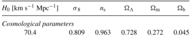
Table 1. Cosmological parameters adopted in our simulations. H0[km s−1Mpc−1] σ8 ns 3 m b Cosmological parameters
70.4 0.809 0.963 0.728 0.272 0.045
Table 2. Mass resolution for dark matter particles, gas cells and star particles, and spatial resolution (in physical units) for our simulations.
Type mcdm mgas 1xmin
(108M⊙h−1] (107M⊙h−1) (kpc h−1) Mass and spatial resolution
Original box 15.5 n.a. 2.14
Zoom-in 1.62 3.22 1.07
within a spherical region of five times their virial radius. In our pre-vious analysis (Martizzi et al.2014), we determined that only 25 of these clusters are relaxed. High-resolution initial conditions were extracted for each of the 51 haloes, with the aim of performing zoom-in re-simulations. We ran three different re-simulations per halo: (I) including dark matter and neglecting baryons, (II) includ-ing dark matter and baryons and stellar feedback, (III) includinclud-ing baryons, stellar feedback and AGN feedback. In this paper, we focus on cases (II) and (III), because they allow us to study the properties of BCGs.
In the re-simulations, the dark matter particle mass is
mcdm= 1.62 × 10⁸M⊙ h−1, while the baryon resolution element
has a mass of mgas = 3.22 × 10⁷M⊙. We set the maximum
re-finement level to ℓ = 17, corresponding to a minimum cell size 1xmin= L/2ℓmax≃ 1.07 kpc h−1. The grid was dynamically
re-fined using a quasi-Lagrangian approach: when the dark matter or baryonic mass in a cell reaches eight times the initial mass reso-lution, it is split into eight children cells. Table2summarizes the particle mass and spatial resolution achieved in our simulations.
We model gas dynamics using a second-order unsplit Godunov scheme (Teyssier2002; Fromang, Hennebelle & Teyssier 2006; Teyssier, Fromang & Dormy2006) based on the HLLC Riemann solver and the MinMod slope limiter (Toro, Spruce & Speares1994). We assume a perfect gas equation of state with polytropic index γ= 5/3. All the zoom-in runs include subgrid models for gas cool-ing which account for H, He and metals and that use the Sutherland & Dopita1993cooling function. We directly follow star formation and supernovae feedback (‘delayed cooling’ scheme, Stinson et al.
2006) and metal enrichment. In the 51 re-simulations, we also in-cluded an AGN feedback scheme, a modified version of the Booth & Schaye (2009) model. In this scheme, supermassive black holes (SMBHs) are modelled as sink particles and AGN feedback is pro-vided in form of thermal energy injected in a sphere surrounding each SMBH. We label these simulations as AGN-ON. The other 51 HYDRO simulations do not include AGN feedback. We label these simulations as AGN-OFF. More details about the AGN feedback scheme can be found in Teyssier et al. (2011) and Martizzi et al. (2012a).
There are a number of unconstrained free parameters in the galaxy formation model we adopt. In particular, the efficiency of the AGN feedback and star formation process are two crucial parameters. A careful study of the tuning of AGN feedback models implemented in theRAMSEScode has been performed by Dubois et al. (2012). In
our case, the tuning has been performed re-simulating one of the haloes in our catalogue (the less massive one) several times while varying the star formation efficiency ǫ∗and the size of the region where the AGN feedback energy is injected. The model that best reproduces the MBH–σ relation and the central galaxy masses has
star formation efficiency ǫ∗= 0.03 and size of the AGN feedback injection region equal to twice the cell size. For the AGN-OFF simulations, we adopt ǫ∗= 0.01, which is close to the lower limit
of the observed star formation efficiencies. However, even with such a low ǫ∗, overcooling is still expected to be very strong in galaxy clusters, leading to BCG properties that disagree with the observations (see following sections).
In a previous study (Martizzi et al.2012a), we showed that AGN feedback plays a relevant role in the evolution of simulated BCGs. The limit of our previous work was that the analysis was limited to one cluster, simulated at very high resolution. The large sample we analyse in this paper constitutes a complementary data set and allows us to test our galaxy formation model in a large number of haloes with different merger histories.
3 P R O P E RT I E S O F T H E S I M U L AT E D B C G S
In this section, we analyse the properties of the BCGs in our sample. Given that approximately half of our simulated clusters are relaxed whereas the other half are unrelaxed, our BCGs should represent a fairly unbiased sample of objects at z = 0. The resolution of our simulations is not adequate for the comparison of the progenitors of the BCGs to high-redshift galaxies. On the other hand, at z = 0, the BCGs are better resolved; therefore, we focus our analysis on the z = 0 properties.
3.1 BCG identification and analysis
BCGs are extremely massive systems sitting close to cluster cen-tres. Since their position can be offset with respect to the cluster centre (see e.g. Mohammed et al.2014), we identify BCG centres separately from halo centres. To accomplish that we ran a mod-ified implementation of AdaptaHOP (Aubert et al.2004; Tweed et al.2009) on the distribution of stellar particle with the aim of identifying galaxy centres. The BCG centres were identified as the centres of the most massive galaxies close to the cluster cores. We use the information provided by AdaptaHOP to remove satellite galaxies from our analysis and keep only the BCG surrounded by its extended stellar halo, i.e. the ICL.
The recent work by Ragone-Figueroa et al. (2013) explores the properties of BCGs in SPH simulations. These authors define BCG masses in several ways and reach qualitatively similar conclusion
for all their mass definitions. Their results show that dynamical decoupling of BCG and ICL is a very accurate procedure to measure BCG stellar masses in simulations (Puchwein et al.2010; Cui et al.
2014); however, when the aim is measuring the integrated properties of BCGs, it is much easier to rely on mock photometric data. For this reason, we base our analysis on mock V-band images of the BCGs in our sample generated using theSUNSETcode included in
theRAMSESpackage.SUNSETis based on a simplified STARDUST
SSP model (Devriendt, Guiderdoni & Sadat1999).
Once the V-band images are generated, we measure surface brightness profiles for all the BCGs. The BCG mass is defined as the projected mass enclosed within the isophotal contour with µV= 25 mag arcsec−2. We ought to stress that this threshold is
one mag arcsec−2fainter than the one adopted by Ragone-Figueroa
et al. (2013); however, this allows us to include stellar mass that might be lost by adopting a lower (brighter) threshold. As a mat-ter of fact, recent studies suggest (Gonzalez, Zabludoff & Zaritsky
2005; Kravtsov, Vikhlinin & Meshscheryakov2014) that the stellar light distribution of BCGs is much more extended than assumed in previous works (see the next section for a discussion on this topic). The outer isophotal contour and the measured stellar mass are then used to estimate half-light radii, velocity dispersions and SFRs for all the BCGs. To avoid biases related to the choice of a line of sight, we repeat the same analysis along 10 random lines-of-sight for each galaxy, then we average the results.
Fig.1shows an edge on image of one of the BCGs in our sample. To make these images, we use the information from the halo finder to remove the contribution from satellite galaxies. The image on the left represents the AGN-OFF case, whereas the image on the right represents the AGN-ON case. Significant differences are noticeable in the luminosity and morphology of the object. The AGN-OFF BCG is much more extended and luminous than the AGN-ON real-ization in the same halo. Furthermore, the AGN-OFF BCG is a disc galaxy, whereas the AGN-ON BCG appears to be a very luminous elliptical galaxy.
In the following sections, we will show direct quantitative com-parison of the two scenarios to observational results. This compar-ison will help in gaining a better understanding of the models and their predictions.
Figure 1. Edge-on view of one of the BCGs in our sample: V-band flux in arbitrary units. Left: AGN-OFF. Right: AGN-ON. The colour scale is the same in both panels. All the satellites have been removed from these images.
3.2 Halo mass versus stellar mass
Successful models of galaxy formation are expected to reproduce the relation between galaxy stellar mass and halo mass. The slope of this relation is not constant, it varies with halo mass (van den Bosch, Yang & Mo2003; Conroy & Wechsler2009; Hansen et al.2009; Moster et al.2010; Behroozi, Wechsler & Conroy2013; Moster, Naab & White2013; Kravtsov, Vikhlinin & Meshscheryakov2014). This fact can be interpreted as evidence that haloes of different masses convert their initial baryonic content into stars at different rates. Traditional galaxy formation models are known to produce gas overcooling in galaxy clusters. This process leads to very efficient conversion of gas into stars, i.e. to SFRs and galaxy masses in excess with respect to those observed cluster galaxies. AGN feedback has been proposed has a mechanism to solve the overcooling problem and the overproduction of stars simultaneously (Springel, Matteo & Hernquist2005; Croton et al.2006; Sijacki et al.2007; Booth & Schaye2009). In this section, we compare the results of our simulations to the most recent halo mass versus stellar mass relations reported in the literature.
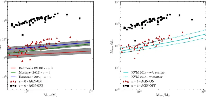
The left-hand panel of Fig.2shows the comparison of our simu-lated BCGs at redshift z = 0 to the halo mass versus stellar mass re-lation obtained using several techniques (Hansen et al.2009; Moster et al.2010,2013; Behroozi et al.2013; Kravtsov et al.2014). AGN-OFF simulations produce central galaxies that are ∼10 times more massive than what is expected to observe in the real Universe. As already mentioned, this is one of the effects of gas overcooling. The AGN-ON results are in much better agreement with the expected halo mass versus stellar mass relation for these massive haloes; however, this result needs to be more carefully analysed. The AGN-ON BCGs tend to match better the relations that predict a higher halo mass (Moster et al.2013). In the low-mass range showed in this plot, our AGN-ON also agree with the results of Behroozi et al. (2013). The differences between the curves from Hansen et al. (2009), Moster et al. (2013) and Behroozi et al. (2013) are caused
by different systematic effects; however, they all lie within 2σ from each other, where σ is the scatter in the halo mass versus stellar mass relation (grey shaded areas in the left-hand panel of Fig.2). Given these consideration and given our mass definition (see Section 3.1), we cannot tell whether the AGN-ON simulations overproduce or underproduce BCG stellar masses.
Kravtsov et al.2014) discuss in detail how abundance matching should be done in the mass range of BCGs: their halo mass versus stellar mass has been obtained by using the recent calibration of the stellar mass function by Bernardi et al. (2013), which is based on accurate fits to the light profiles of the most luminous galax-ies. For BCGs this means fitting the light profiles to distances up to ∼100–200 kpc from their centre. Such distance is ∼4–5 times more extended than the one usually adopted to define BCG sizes, and is likely to include part of the ICL in the central object mass budget. This leads to the increased stellar mass values observed in the stellar mass versus halo mass relation that we also show in the right-hand panel of Fig.2. Therefore, the mass definition based on the µV= 25 mag arcsec−2threshold is not adequate for
compar-ison to Kravtsov et al.2014), because it underestimates the mass in the BCG+ICL component. With the aim of studying the effect of adopting a given surface brightness threshold, we carefully in-spected the relationship between mass profiles and light profiles in our simulations.
The left-hand panel of Fig.3shows the surface brightness profiles of the AGN-ON and AGN-OFF BCG. Most of the light is concen-trated within the µV = 25 mag arcsec−2 limit; however, there is
still a significant amount of light outside of this region out to ∼60– 100 kpc. To measure the amount of mass that is missed by an ob-servation with a given surface brightness limit, we plot the enclosed stellar mass normalized to the total stellar mass in BCG+ICL as a function of the surface brightness limit adopted in the right-hand panel of Fig.3. The total stellar mass in BCG+ICL is obtained by
removing the stellar mass in the satellite galaxies using information
Figure 2. Left: results from our simulations versus the halo mass versus stellar mass relation at redshift z = 0 fromHansen et al. (2009, blue line, with its 1σ scatter), Moster et al. (2013, green line), Behroozi et al. (2013, red line, with its 1σ scatter). Our AGN-ON simulations are represented by the red triangles, whereas the AGN-OFF simulations are represented by black squares. The BCG stellar mass definition assumes a surface brightness limit µV= 25 mag arcsec−2. Right: halo mass versus stellar mass relation at redshift z = 0 from Kravtsov et al.2014, cyan line) versus our simulations. Our AGN-ON simulations are represented by the red triangles, whereas the AGN-OFF simulations are represented by black squares. The stellar mass on the y-axis is the total stellar mass associated with the BCG+ICL component.
Figure 3. Left: V-band surface brightness for all the BCGs in our sample. AGN-ON is shown in red, AGN-OFF is shown in black. The green dashed line represents the surface brightness cut adopted to define galaxy masses µV = 25 mag arcsec−2. The blue dashed line represents an alternative cut µV= 27 mag arcsec−2which allows us to include most of the ICL in the stellar mass estimate. Right: normalized stellar mass as a function of the adopted magnitude cut for all the BCGs. The mass distribution includes BCG+ICL. The green and blue lines represent µV= 25 mag arcsec−2and µV= 27 mag arcsec−2, respectively.
from the halo finder. The AGN-OFF galaxies are much more cen-trally concentrated, so most of the mass (∼80–90 per cent) is still enclosed in the isophotes with µV<25 mag arcsec−2. In the
AGN-ON case, the stellar mass distribution is less centrally concentrated and the BCGs have a very extended ICL. As a result, very high µVvalues are needed to be able to observe the ICL mass. A limit
µV= 25 mag arcsec−2might be adequate to capture the mass of the
BCG, but not the entire mass of the BCG+ICL. Our results show that µV= 25 mag arcsec−2captures only ∼10–60 per cent of the
total stellar mass. A surface brightness limit µV= 27 mag arcsec−2
gives 40–80 per cent of the total stellar mass in BCG+ICL. If we use the total stellar mass in BCG+ICL and compare to Kravtsov et al.2014), we get the result in the right-hand panel of Fig.2: the match of our simulations to these results is excellent. This result is non-trivial since the Kravtsov et al.2014) masses are obtained by extrapolating their multiple S´ersic fits to high radii. Fig.4shows normalized surface density profiles for the AGN-ON BCGs com-pared to those of the observed BCGs of Kravtsov et al. 2014). Radius has been normalized with respect to R500c, surface density
has been normalized with respect to the half-mass surface density 61/2= 0.5M∗,tot/4πR1/22 , where R1/2is the BCG+ICL half-mass
radius and M∗, totis the stellar mass in BCG+ICL. Fig. 4shows that the extrapolation of the profiles in the observational sample closely matches the profiles of the simulated BCGs at high radii. This implies that our simulations closely match observations and that extrapolation of fitted surface density profiles (triple S´ersic functions in this case) are sufficiently robust to be used to measure stellar masses.
4 OT H E R P R O P E RT I E S O F T H E S I M U L AT E D B C G S
In this section, we compare the properties of the simulated BCGs obtained by integrating the information within the half-light radius. We define the half-light radius as the radius containing half
Figure 4. Normalized surface density profiles of the AGN-ON BCGs (red lines) compared to those of the observed BCGs of Kravtsov et al.2014). Solid black lines represent the fits in the region where the profiles have been measured, dashed black lines represent the fits in the regions where the profile has been extrapolated.
of the luminosity of the BCG within the isophote with µV <
25 mag arcsec−2. The stellar mass of the BCG has been measured by
using the criterion described in the previous section. SFRs have been measured considering only the stars formed in the latest 5 × 10⁸yr.
Half-light radii, velocity dispersions, stellar masses are compared to the values found in observations. We measure these parameters by averaging over several lines of sight per galaxy. The goal of
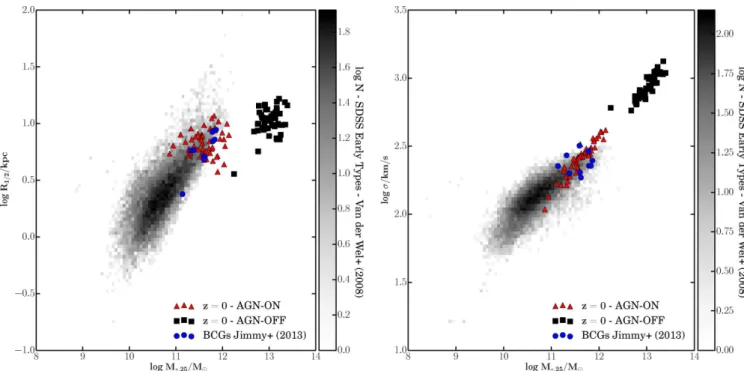
Figure 5. Left: stellar mass versus size. The size is the half-light radius for the simulated BCGs and the effective radius for the observational data. Right: Stellar mass versus stellar velocity dispersion. The shaded area represents galaxy counts per bin from the ETG sample by Van der Wel et al. (2008) sample from SDSS. The blue circles are the BCGs analysed by Jimmy et al. (2013).
such comparison is to test the galaxy formation prescriptions and to identify discrepancies with the observations that point at evident flaws in the model.
The left-hand panel of Fig.5shows the stellar mass versus size re-lation at z = 0 for the simulated BCG compared to that found by van der Wel et al. (2008) for a sample of early-type galaxies extracted from the Sloan Digital Sky Survey (SDSS) and to the recent data published by Jimmy et al. (2013). A similar comparison is shown in the right-hand panel of the same figure but for the stellar mass versus velocity dispersion relation. As we already know from the analysis in the previous section, the masses of the AGN-OFF BCGs are one order of magnitude larger than the ones of massive galaxies observed in the real Universe. Fig.5also shows that the AGN-OFF galaxies are also larger, have much higher velocity dispersion and are more centrally concentrated than the AGN-ON galaxies. Gas overcooling leads very efficient gas fuelling of the BCG and to high SFRs in disc structures (see the left-hand panel of Fig1); due to the large amount of baryonic matter in their central regions, these BCGs become more centrally concentrated and obtain huge velocity dis-persions. On the other hand the AGN-ON BCGs show a remarkable agreement in mass, size and velocity dispersion compared to the most massive early-type galaxies in van der Wel et al. (2008) and to the BCGs in Jimmy et al. (2013). A small discrepancy can be noticed between the sizes of the most massive BCGs and those of the early-type galaxies which could point at some flaw in the model that manifests its effects only in the most massive haloes. However, we cannot draw a definitive conclusion on the actual existence of this discrepancy since it is known that the most massive BCGs are not scaled-up versions of elliptical galaxies (von der Linden et al.
2007).
Interesting results are found when we compare the stellar mass versus SFR relation at z = 0 for the simulated BCGs to the data of Liu, Mao & Meng (2012, SFRs of early-type BCGs measured from their Hα emission, SDSS data), as shown in Fig. 6. AGN-OFF galaxies have SFRs too high by a factor 5–10 with respect
Figure 6. Stellar mass versus SFR for the ‘star-forming’ BCGs. The sim-ulations are compared to the observational data by Liu et al. (2012, green squares). The BCGs with reported SFR < 10−1M
⊙yr−1are represented by upper limits (the measured SFR is 0 M⊙yr−1). The blue solid line rep-resents a power-law extrapolation of the sequence for star-forming galaxies measured byBrinchmann et al. (2004).
to the most intensely star-forming BCGs in the Liu et al. (2012) sample. The AGN-ON BCGs show an interesting dichotomy: most of these galaxies have extremely low SFRs shown as upper lim-its in the figure (SFR < 10−1
M⊙ yr−1), i.e. they are completely
quenched BCGs; a secondary population of ‘star-forming’ BCGs is also observed, in remarkable agreement with the data of Liu et al.
(2012). The BCGs with the highest SFRs are close to the sequence of star-forming galaxies at redshift z = 0 (the blue line in Fig.6is an extrapolation of the Brinchmann et al.2004results in the shown mass range). The prescription adopted for the AGN scheme allows for late mild star formation events in BCGs, typically in the cluster with the most un-relaxed central regions. This star-forming activity is likely to be a transient and to be suppressed by AGN feedback bursts of activity, since the gas accretion required for star formation also feeds the central SMBH and will trigger an AGN burst. The dichotomy between mildly star-forming and quenched BCGs is ob-served also in the most massive BCGs which sit in the most massive haloes. Despite this qualitative match with observations, the frac-tion of star-forming BCGs in the simulated sample is ∼50 per cent, higher than the fraction measured by Liu et al. (2012) for an X-ray selected sample (∼20 per cent). This discrepancy between obser-vations and simulations and might be interpreted as a limit of the subgrid model we adopt for AGN feedback.
Finally, we compare the kinematic properties of the simulated objects to those of observed BCGs at redshift z = 0. One of the most interesting plots for early-type galaxies is the ǫ–λR(Emsellem et al.
2007,2011), typically studied using integral field spectroscopy: ǫ is the galaxy ellipticity, λRis a parameter that quantifies the angular
momentum content in galaxies, it has been specifically defined to be measured from integral field spectroscopy and it is defined as λR= hR|V |i
hR√V2+ σ2i, (1)
where V is the line-of-sight velocity in a pixel, σ is the velocity dispersion in the pixel, R is the distance of the pixel from the centre and the brackets represent an average over all the pixels. Low values of λRare associated with slowly rotating galaxies (slow rotators),
high values of λR are associated with fast rotating galaxies (fast
rotators). We measure the value of λRwithin the half-light radius
and the edge-on ellipticities of the simulated BCGs, then com-pare our results to the BCGs observed by Jimmy et al. (2013). We ought to stress that Jimmy et al. (2013) report apparent ellipticities and that they measure λRwithin the effective radius. Despite these
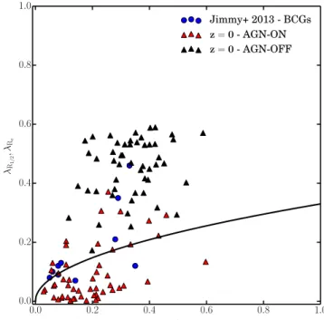
differences between the measurement method, observational uncer-tainties are still large enough to allow a meaningful comparison of data and simulations. The comparison of the simulated BCGs to the Jimmy et al. (2013) data is shown in Fig.7. The black solid line λR∝√ǫrepresents the separation between fast and slow rotators
(Emsellem et al. 2011). The AGN-OFF population is exclusively composed of fast rotators in contrast with the properties of real BCGs. These AGN-OFF BCGs possess very massive rotating disc components. On the other end, the AGN-ON BCGs show a variety of kinematic properties that is observed also in the Jimmy et al. (2013): both fast and slow rotators are produced. If we assume Poisson error bars, the fast-to-slow rotators ratio in the AGN-ON sample is ∼0.29, whereas it is ∼33 per cent in the Jimmy et al. (2013) sample. The fast-to-slow rotators ratio of AGN-ON BCGs is consistent with the observed one within the observational uncer-tainty. However, some considerations are needed before drawing conclusions. First of all, the size of the Jimmy et al. (2013) sample is quite small and comparison to additional data samples needs to be performed (e.g. GAMA; Oliva-Altamirano et al.2014or future surveys like MASSIVE). Secondly, the kinematic structure of the less massive BCGs in our simulations could be better resolved in higher resolution simulations like the one analysed in Martizzi et al. (2012a). Unfortunately, running one of these simulations requires roughly the same amount of computational resources as the entire sample analysed here. Thirdly, the strategy we adopted to select
Figure 7. Ellipticity (edge-on view) versus angular momentum probe parameter λR measured within the half-light radius. This plot is used to separate fast rotators and slow rotators; here, the separation is represented by the black solid line λR= 0.33 ∗√ǫ. Values measured within the effective radius of a sample of real BCGs from Jimmy et al. (2013) are also compared to our results (blue circles). The Jimmy et al. ellipticities are apparent and have not been corrected.
the haloes for the zoom-in simulations might introduce a bias in the selection of fast versus slow rotators. We will carefully explore these issues in future work.
4.1 Comparison to previous literature
The formation of BCGs has been studied from a theoretical view-point by several authors who identified some of the main elements that drive the formation of these extremely massive galaxies. Dubin-ski (1998) explored the problem of forming a very massive galaxy at the centre of a cluster using N-body simulations finding that merg-ers of several massive galaxies can lead to the formation of a large BCG. More recently, Conroy, Wechsler & Kravtsov (2007) stud-ied the build-up of BCGs and ICL and the evolution of the galaxy mass function between redshift z = 1 and z = 0, concluding that a large fraction (∼80 per cent) of the stars from disrupted haloes in a cluster end up contributing to the ICL. De Lucia & Blaizot (2007) studied the evolution of BCGs using semi-analytical modelling and concluded that most of their mass is assembled at redshift z > 1 by rapid cooling flows which are later suppressed by AGN feedback. In our previous paper (Martizzi et al.2012a), we analysed the prop-erties of the BCG formed at the centre of a 1014
M⊙ cluster with a better resolution than the one we achieve in this paper (minimum cell size 1x ∼ 0.5 kpc, dark matter mass particle ∼8 × 10⁶
M⊙). Our previous results are basically consistent with those we show in this paper.
An interesting comparison can be made with the results of Ragone-Figueroa et al. (2013) which performed an analysis very similar to the one done in this paper, but used SPH-based cosmo-logical simulations. The resolution achieved in this work (softening length 2.5 kpc h−1, dark matter particle mass ∼8 × 10⁸
slightly worse, but comparable to the one we achieve in this paper. Their implementation of AGN feedback is very similar to the one we adopt. Their conclusion is that AGN feedback is too efficient in the central regions of galaxies, generating density profiles with cores at their centre (see also Martizzi et al.2012band Ragone-Figueroa et al.2012), but generally inefficient at reducing the global star for-mation in the most massive galaxies. The flattening of the density profiles is observed in both SPH and AMR simulations and is likely a feature produced by implementations of AGN feedback in form of thermal energy. In simulations, such flattening is measured at the scale of 5–10 kpc, but it is quite rare to observe flat density pro-files in real elliptical galaxies at a scale larger than 3 kpc (Postman et al.2012). This is an indication that this kind of implementation of AGN feedback is indeed too efficient at small scales. However, we do not find strong discrepancies in BCG masses as reported in Ragone-Figueroa et al. (2013). This difference might be related to intrinsic differences between SPH and AMR codes in the way gas of different phases mixes. This fact might influence the way gas cools, forms stars and accretes on SMBHs. Additionally, it is not guaranteed that implementations of the same subgrid model work in the same way in an SPH and in an AMR code. These issues could be explicitly addressed by performing a dedicated code comparison project.
5 S U M M A RY A N D C O N C L U S I O N S
In this paper, we have analysed the low-redshift properties of a sample of BCGs formed at the centre of 51 galaxy clusters simulated with the AMR codeRAMSES. The zoom-in technique is adopted to
obtain the required resolution only in the region surrounding each cluster, allowing us to save computing time. Several properties of the BCGs have been analysed, with the aim of testing the galaxy formation models adopted for the simulations. A similar analysis on AMR simulations has been shown in Martizzi et al. (2012a); however, here we focus for the first time on much larger sample of AMR simulations of cluster evolution and BCG formation. One of the crucial effects needed to reproduce the properties that match those of real BCGs is a source of heating that slows down the cooling of large quantities of gas in massive galaxies, therefore quenching star formation. In this paper, we specifically focus on the effect of AGN feedback as the heating source. The feedback scheme is very simple (it is largely inspired by Booth & Schaye2009), so that careful comparison to observation can lead to the identification of its limits.
The results of this analysis can be summarized in a few points: (i) Simulations without AGN feedback do not reproduce the properties of observed BCGs. The simulated objects appear to be too massive, too large, too centrally concentrated and they are all fast rotators.
(ii) Including AGN feedback reduces stellar masses and velocity dispersions. Galaxy half-light radii are only weakly modified. The properties of this population of simulated BCGs are very similar to those of real BCGs observed at redshift z = 0. There are some small discrepancies only for the most massive BCGs.
(iii) The BCGs simulated in the presence of AGN feedback are surrounded by a very extended ICL (up to a few ∼100 kpc from the centre) that accounts for 20–60 per cent of stellar mass associated with the total BCG+ICL component. A significant fraction of the ICL can be detected only by deep observations which probe regions of surface brightness µV>27 mag arcsec−2. However, to detect the
whole component even deeper observations are needed.
(iv) The objects in our sample match well the halo mass versus stellar mass relation even when the comparison is performed by accounting for the total mass in BCG+ICL as in Kravtsov et al.
2014).
(v) Approximately half of the BCGs simulated in presence of AGN feedback are completely quenched early-type objects. How-ever, some of the BCGs form stars at rates similar to those in observed star-forming BCGs (Liu et al.2012). The fraction of star-forming BCGs is a factor ∼2 lower in X-ray selected observational samples. This fact might be considered as an effect of partially in-efficient quenching of star formation from the subgrid model we adopt for AGN feedback.
(vi) The BCGs simulated in the presence of AGN feedback are di-vided between fast and slow rotators as in the real Universe (Brough et al.2011; Jimmy et al.2013). The comparison made in this paper shows that the fast-to-slow rotator fraction in the simulated sample is consistent with that measured by (Jimmy et al.2013); however, this result needs to be updated by considering large observational data samples and simulations with improved resolution.
The simple prescription for AGN feedback we adopted manages to solve the most critical problem for the formation of BCGs: gas overcooling triggering excessive star formation at z < 1. Given its simplicity (spherical symmetry of AGN activity, simple accretion rate formulae for SMBHs, lack of kinetic energy injection or jets, etc.), the model produces BCGs that closely match those in the real Universe. The match appears to be somewhat worse when only the most massive BCGs are considered and the ratio of star-forming to non-star-forming BCGs is too high. At the moment, we cannot assess whether these discrepancies at the high-mass end are caused by missing physical processes that might be relevant in galaxy clus-ters (anisotropic thermal conduction, jets, cosmic ray streaming). As time is needed before having larger observational samples of BCGs to carry out extensive comparison projects, there are at least two approaches to continue testing this particular galaxy forma-tion framework. First, a fair sample of simulaforma-tions with improved resolution might be needed to study the kinematics and formation histories of the most massive BCGs in the range of masses in which the largest discrepancies are observed. Secondly, a detailed analy-sis of the gas properties and accretion histories might be relevant because it will allow us to quantify the exact condition in which over-cooling is still a problem and to directly compare to e.g. X-ray data. Given its relevance and need for careful discussion, we plan to perform this separate analysis in future work.
AC K N OW L E D G E M E N T S
The simulations have been run on the Monte Rosa cluster at CSCS, Switzerland. DM is working as a postdoctoral fellow at University of California at Berkeley and his work is funded by the Swiss National Science Foundation. We thank Andrey Kravtsov for the useful discussions that improved the quality of this paper. We also thank our anonymous referee for his comments which helped us clarifying some critical points in the paper.
R E F E R E N C E S
Aubert D., Pichon C., Colombi S., 2004, MNRAS, 352, 376 Behroozi P. S., Wechsler R. H., Conroy C., 2013, ApJ, 770, 57
Bernardi M., Meert A., Sheth R. K., Vikram V., Huertas-Company M., Mei S., Shankar F., 2013, MNRAS, 436, 697
Bertschinger E., 2001, ApJS, 137, 1
Brinchmann J., Charlot S., White S. D. M., Tremonti C., Kauffmann G., Heckman T., Brinkmann J., 2004, MNRAS, 351, 1151
Brough S., Tran K.-V., Sharp R. G., von der Linden A., Couch W. J., 2011, MNRAS, 414, L80
Conroy C., Wechsler R. H., 2009, ApJ, 696, 620
Conroy C., Wechsler R. H., Kravtsov A. V., 2007, ApJ, 668, 826 Croton D. J. et al., 2006, MNRAS, 365, 11
Cui W. et al., 2014, MNRAS, 437, 816
Devriendt J. E. G., Guiderdoni B., Sadat R., 1999, A&A, 350, 381 Dubinski J., 1998, ApJ, 502, 141
Dubois Y., Devriendt J., Slyz A., Teyssier R., 2012, MNRAS, 420, 2662 Eisenstein D. J., Hu W., 1998, ApJ, 496, 605
Emsellem E. et al., 2007, MNRAS, 379, 401 Emsellem E. et al., 2011, MNRAS, 414, 888 Fabian A. C., 2012, ARA&A, 50, 455
Fromang S., Hennebelle P., Teyssier R., 2006, A&A, 457, 371 Gonzalez A. H., Zabludoff A. I., Zaritsky D., 2005, ApJ, 618, 195 Gonz´alez M., Audit E., Huynh P., 2007, A&A, 464, 429
Hansen S. M., Sheldon E. S., Wechsler R. H., Koester B. P., 2009, ApJ, 699, 1333
Jimmy Tran K.-V., Brough S., Gebhardt K., von der Linden A., Couch W. J., Sharp R., 2013, ApJ, 778, 171
Kravtsov A., Vikhlinin A., Meshscheryakov A., 2014, preprint (arXiv:e-prints)
Liu F. S., Mao S., Meng X. M., 2012, MNRAS, 423, 422 Lucia G. D., Blaizot J., 2007, MNRAS, 375, 2
McCarthy I. G., Schaye J., Bower R. G., Ponman T. J., Booth C. M., Dalla Vecchia C., Springel V., 2011, MNRAS, 412, 1965
McConnell N. J., Ma C.-P., 2013, ApJ, 764, 184
Martizzi D., Teyssier R., Moore B., 2012a, MNRAS, 420, 2859 Martizzi D., Teyssier R., Moore B., Wentz T., 2012b, MNRAS, 422, 3081 Martizzi D., Mohammed I., Teyssier R., Moore B., 2014, MNRAS, 440,
2290
Mohammed I., Liesenborgs J., Saha P., Williams L. L. R., 2014, MNRAS, 439, 2651
Moster B. P., Somerville R. S., Maulbetsch C., van den Bosch F. C., Macci`o A. V., Naab T., Oser L., 2010, ApJ, 710, 903
Moster B. P., Naab T., White S. D. M., 2013, MNRAS, 428, 3121 Oliva-Altamirano P. et al., 2014, MNRAS, 440, 762
Postman M. et al., 2012, ApJ, 756, 159
Puchwein E., Springel V., Sijacki D., Dolag K., 2010, MNRAS, 406, 936 Ragone-Figueroa C., Granato G. L., Abadi M. G., 2012, MNRAS, 423, 3243 Ragone-Figueroa C., Granato G. L., Murante G., Borgani S., Cui W., 2013,
MNRAS, 436, 1750
Rudick C. S., Mihos J. C., Harding P., Feldmeier J. J., Janowiecki S., Morrison H. L., 2010, ApJ, 720, 569
Sijacki D., Springel V., Matteo T. D., Hernquist L., 2007, MNRAS, 380, 877
Springel V., Matteo T. D., Hernquist L., 2005, ApJ, 620, L79
Stinson G., Seth A., Katz N., Wadsley J., Governato F., Quinn T., 2006, MNRAS, 373, 1074
Sutherland R. S., Dopita M. A., 1993, ApJS, 88, 253 Teyssier R., 2002, A&A, 385, 337
Teyssier R., Fromang S., Dormy E., 2006, J. Comput. Phys., 218, 44 Teyssier R., Moore B., Martizzi D., Dubois Y., Mayer L., 2011, MNRAS,
414, 195
Toro E. F., Spruce M., Speares W., 1994, Shock Waves, 4, 25
Tweed D., Devriendt J., Blaizot J., Colombi S., Slyz A., 2009, A&A, 506, 647
van den Bosch F. C., Yang X., Mo H. J., 2003, MNRAS, 340, 771
von der Linden A., Best P. N., Kauffmann G., White S. D. M., 2007, MNRAS, 379, 867
van der Wel A., Holden B. P., Zirm A. W., Franx M., Rettura A., Illingworth G. D., Ford H. C., 2008, ApJ, 688, 48
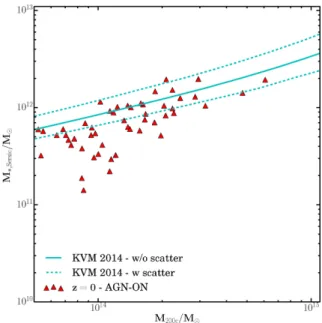
A P P E N D I X A : S T E L L A R M A S S V E R S U S H A L O M A S S W I T H S ´E R S I C F I T S
We have tried several definitions for the stellar mass we plot in Fig.2. In this appendix, we show the results we obtain when we adopt an alternative mass definition with respect to the one shown in the main text. Since the differences are not huge, we only show the results here. A straightforward approach to obtain stellar masses from simulations is to fit the surface brightness profiles with an analytical function. After excluding the satellite galaxies from the analysis, we fit a double S´ersic profile (the sum of two Service profiles) to the BCG+ICL component. We find that a double S´ersic function is generally an excellent fit to the simulated data. We as-sociate the BCG to the inner stellar component, we estimate its stellar mass and we plot it against the halo mass in Fig.A1. For the most massive haloes, the stellar masses obtained with this pro-cedure are slightly larger than the ones obtained by adopting the surface brightness cut; however, the difference is somewhat smaller for the less massive haloes.
Figure A1. Results from our simulations versus the halo mass versus stellar mass relation at redshift z = 0 from KVM 2014. Our AGN-ON simulations are represented by the red triangles. The BCG stellar mass definition is based on double S´ersic fits.