iSpectra: An Open Source Toolbox For The Analysis of Spectral Images Recorded on Scanning Electron Microscopes

© MICROSCOPY SOCIETY OF AMERICA 2015

iSpectra: An Open Source Toolbox For The Analysis of

Spectral Images Recorded on Scanning Electron

Microscopes

Christian Liebske*

Department of Earth Sciences, Institute of Geochemistry and Petrology, ETH Zürich, Sonneggstrasse 5, 8092 Zürich, Switzerland

Abstract: iSpectra is an open source and system-independent toolbox for the analysis of spectral images (SIs) recorded on energy-dispersive spectroscopy (EDS) systems attached to scanning electron microscopes (SEMs). The aim of iSpectra is to assign pixels with similar spectral content to phases, accompanied by cumulative phase spectra with superior counting statistics for quantification. Pixel-to-phase assignment starts with a threshold-based pre-sorting of spectra to create groups of pixels with identical elemental budgets, similar to a method described by van Hoek (2014). Subsequent merging of groups and re-assignments of pixels using elemental or principle component histogram plots enables the user to generate chemically and texturally plausible phase maps. A variety of standard image processing algorithms can be applied to groups of pixels to optimize pixel-to-phase assignments, such as morphology operations to account for overlapping excitation volumes over pixels located at phase boundaries. iSpectra supports batch processing and allows pixel-to-phase assignments to be applied to an unlimited amount of SIs, thus enabling phase mapping of large area samples like petrographic thin sections. Key words: energy-dispersive spectroscopy, spectral imaging, phase mapping, scanning electron microscopy, image morphology

I

NTRODUCTION

Modern scanning electron microscopes (SEMs) are often equipped with energy-dispersive spectroscopy (EDS) systems for chemical analysis. Such systems are usually supplied with software to acquire and subsequently analyze so-called spectral or spectrum images for elemental or phase mapping purposes. Spectral images (SIs) can be envisioned as 3D arrays where the X–Y plane corresponds to image coordinates on the sample surface and data in the Z direction contain an energy-dispersive spectrum of the specimen at each XY position, saved as intensity per channel with a constant increment in energy (see e.g., Friel & Lyman, 2006 for a review of X-ray mapping techniques in micro-beam analysis.)

Compared with more conventional element mapping on electron probe micro-analyzers with wavelength-dispersive spectrometers, where the elements of interest must be selected before the start of the measurement, EDS spectral imaging does not require any foreknowledge of the sample chemistry as the entire spectrum, defined by the response of the sample to accelerated electrons, is recorded. This has several implications: it allows off-line analysis of the sample such that spectra of user-defined regions of interest (ROIs) can be extracted and quantified, mapping of elements that may not have been con-sidered beforehand, but it also allows phase maps to be created by sorting and grouping pixels according to spectral contents.

The success in creating phase maps depends on the counting statistics of the SI, which is greatly supported by the

use of modern Si-drift detectors, but equally important on the ability of the software to recognize chemically distinct features. Most commonly, this problem is approached by applying algorithms for multivariate statistical analysis to detect principle components, which serve as the basis for pixel-to-phase assignments (e.g., Bonnet et al., 1992; Kotula et al., 2003; Parish, 2011; Lucas et al., 2013). Such methods have the advantage of an un-biased, objective and user-friendly procedure; on the other hand, such algorithms have generally no understanding of chemical or textural patterns. It is important to distinguish between groups of pixels with similar spectral features and groups of pixels that represent phases. The chemical compositions and textures (i.e., grain shapes and sizes and inter-granular relationships) of phases are required to interpret the chemical and microstructural characteristics of a sample. The two categories of aforementioned pixels may form an intersecting set but must not necessarily be identical: for example, a zoned mineral may be broken down into pixels covering the chemically distinct zones; however, in order to determine the integrated chemical composition of this mineral (e.g., for mass balance purposes), the pixels covering the entire mineral are of interest. Thus, depending on the purpose of the analysis, such pixels should be grouped differently. This implies that actual user input is indispensible for satisfactory and plausible pixel-to-phase assignment. An additional complexity arises from the inevitable presence of mixed pixels, e.g. image pixels that contain spectral information of more than one phase, which occurs on pixels located at phase boundaries. Such pixels do not belong to any phase and procedures must be established to consider such effects.

*Corresponding author. [email protected] Received November 18, 2014; accepted June 10, 2015

This paper presents iSpectra, a toolbox for the analysis of SIs. iSpectra is written under the premise that it should (1) be“vendor” independent and usable with SI data from a range of EDS hardware systems; (2) give easy access to every spectrum stored in the SI; (3) enable phase mapping in a fully transparent way, avoiding any black-box behavior; (4) allow batch processing to be applied to generate large-scale phase maps; and (5) provide a way for customized, user defined output, which avoids any restrictions that are given by the closed-system nature of “native” EDS software packages, which are delivered with the hardware, thus making use of an open source philosophy. iSpectra applies methods of the recently developed PARC method (PhAse Recognition and Characterization) described by van Hoek et al. (2011) and van Hoek (2014), and adds tools for visualization of chemical features and optimization of pixel assignments.

iSpectra is a collection of user-defined functions written in IGOR Pro (hereafter IGOR; see www.wavemetrics.com), which are accessible via an easy-to-use graphical user interface (GUI). IGOR, being available for Windows and Mac OS X platforms, is a program for scientific graphing, data and image analysis that supports multidimensional arrays (in IGOR terms“waves”), such as 3D SIs, and contains a large number of operations on wave arithmetic and analysis, including fun-damental image processing algorithms. A built-in program-ming environment allows easy scripting of reoccurring tasks and creating GUIs that can be seamlessly integrated into the host program for user-defined applications. iSpectra is written such that it is operable without specific knowledge of the host software IGOR, however, intermediate to advanced IGOR users may modify iSpectra and change its behavior while working on data sets. This paper refers to iSpectra version 2.0. This and the latest version, a comprehensive user manual and sample data can be requested from the author or found on http://www.igorexchange.com/project/iSpectra.

I

S

PECTRA

F

UNCTIONALITY AND

T

OOLS

Supported Data

iSpectra presently contains an import routine for data sets saved in Lispix format (Bright, 1987, see http://www.nist. gov/lispix/). Lispix data sets consist of an uncompressed binaryfile containing all spectra in a consecutive sequence and an accompanying textfile with information on the SI dimensions and data type. The import routine is based on IGOR’s built-in file loading operations, which support a variety offile and data types, such that SIs, saved in different formats, may be loaded after adding additional import functions or modifying existing ones. Data sets saved in uncompressed binary or delimited text formats are readable by IGOR and are thus suitable for analysis in iSpectra.

Loading SIs, Pre-Processing, and Displaying Options

When importing an SI, element maps, i.e. the raw X-ray counts at each image pixel for predefined elements, are being

extracted. iSpectra does not perform peak fitting, and will thus not deconvolute overlapping peaks, but will only extract counts for a specified element, i.e. averaged intensities over the channel of theoretical peak position for a given elemental emission line plus the previous and next channel. Working with a predefined list of elements implies that count peaks of elemental energies that were not included in the initial element list are invisible in the following pixel-to-phase assignment (see Discussion section). To identify undefined energies, a “maximum pixel spectrum” method according to Bright & Newbury (2004) is implemented, such that a spectrum can be generated, which consists of the maximum X-ray counts for each energy channel found in the SI. Comparing this spectrum with the initially defined elemental energies easily reveals missing emission energies. The default list of elements can be altered or a custom list of elements and their X-ray emission energies of the lines of interest can be loaded. The import operation thus results in individual X-ray intensity maps for all specified elements, which are stored in memory as 2D arrays. Most subsequent actions to assign pixels to phases are based on such elemental maps.

The extracted element maps form the basis for principle component analysis (PCA), resulting in a number of “prin-ciple component maps” (PCMs), which are generated as follows. All 2D element maps are rearranged into 1D arrays in a column-priority order and subsequently concatenated into a m × n matrix A, where row m corresponds to the number of pixels in the SI and column n refers to the number of elemental maps. The arithmetic mean is subtracted from each column n ofA to form a data matrix D. Singular value decomposition is then used to decomposeD into n positive eigenvalues (the squares of the singular values) and an n × n eigenvector matrixC. Multiplying C with the transpose of D results in an n × m matrix P. Each row of P represents a projection of each pixel onto an eigenvector, or principle component. Extracting a row from P with m entries and rearranging it into an image matrix results in a PCM. This image resembles a degree of variance of element counts in the SI and provides a way for visualizing chemical variability. The rows inP are ranked in order of decreasing importance, thus, the first row is associated with the first and largest eigenvalue, which, when the latter is divided by the sum of all eigenvalues, equals a fraction of the total variance within matrixD. iSpectra will extract as many PCMs until a certain cumulative variance percentage associated with such images (the default value is >99%) is reached. The default image-display after data import is the PCM associated with the largest variance (Fig. 1a1). Inspection of PCMs related with

1

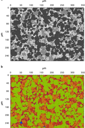
The specimen used as an example in the iSpectra Functionality and Tools section is a run product retrieved from a melting experiment on a peridotitic rock (with a chemical composition representing the Earth’s mantle) performed at 1 GPa pressure and a temperature of 1,250°C. The experiment simulates the generation of basaltic magmas, i.e. produces different silicate minerals in equilibrium with a liquid of basaltic composition, which is quenched to a glass at the end of the experiment. The SI with a dimension of 512 × 384 pixel and a step size of 0.7µm/pixel was acquired on the Thermo Scientific NORAN System attached to Jeol JSM-6390 LA electron microscope with an LaB6 filament at 15 kV.

low variances can be useful to locate chemical features at minor or trace abundance levels.

Further image display options include a“sum image” in which cumulative X-ray counts for each pixel are used as gray values, or RGB maps where each of the extracted element maps can be used as red, green, or blue channel of an RGB color image. The GUI provides a tool for changing element maps to any of the RGB channels for a quick survey of the chemical complexity of the sample (Fig. 1b). Lastly, iSpectra allows an electron microscope image in TIF format (tagged image file) to be loaded, which may be acquired before or during the record of a SI on any of the SEM ima-ging detectors (hereafter SEM image). If this image was recorded at a different image resolution compared with the SI, it will be rescaled to match the latter.

Either of the PCM, sum-, SEM-, or RGB image can be selected as a“base-image” for overlaying colored groups of pixels. Clicking on any pixel of the base-image (regardless of its nature) reveals the raw or background-filtered spectrum (see below) at that pixel location.

Pixels-To-Phase Assignment

The pixel-to-phase assignment is carried out by the user, however, iSpectra as a toolbox provides various instruments and automatic modes to assist. The automatic modes are written under the premise that they should be as transparent as possible to avoid any black-box behavior. This implies that the user has full control, but also full responsibility, over parameters that are being used in such modes.

The initial step is a threshold based, automated group assignment (auto-search), which is carried out in a similar way as described by van Hoek (2014). Two threshold values, a low energy cut-off and a count intensity limit, are applied in the following way: the count number at each given pixel coordinate of any elemental intensity map with energies above the low energy cut-off is compared with the count intensity threshold limit. An element is being recognized at a pixel location if the counts exceed the threshold limit. This results in a list of elements considered to be present at a given pixel location. In the following, this list of elements is also referred to as the pixels elemental budget. A third threshold, a minimum pixel value, merges any group with less pixels into a predefined group “trash,” which serves as a bin for unassigned pixels. The minimum pixel threshold is useful when in a later step an erosion morphologyfilter is applied to account for overlapping excitation volumes at phase boundaries (see details below). The nature of that filter is such that groups with <9 pixels will vanish. Setting the minimum pixel threshold to this value is therefore a logical choice.

The “auto-search” mode can be applied either on raw count or background-filtered intensities. The optional backgroundfiltering is achieved by applying a simple top-hat filter (Schamber 1977; Statham 1977) to all pixel spectra. The channel width of the filter can be made energy dependent and is adjustable on an interactive spectrum graph. Negative contributions of thefiltered spectrum are set to 0. Working on background-filtered spectra is advantageous because the count threshold can be set low while still largely avoiding noise detection, specifically in the 1–3 keV range, where the continuum may be relatively high compared with peaks at higher energies. The principle of auto-search, applied to a background-filtered spectrum, is depicted in Figure 2. The low energy cut-off value and the count threshold limit, shown as blue dashed lines, are being applied to a background-filtered spectrum. Thus, the elemental budget for this pixel and the given threshold values consists of Mg, Al, and Cr (all defined by Kα energies).

Pixels with the same elemental budget are automatically summarized into groups and are displayed as a colored overlay onto the base-image.

Figure 1. Displaying options to represent the 3D spectral image (SI). a: The default image-display is a“principle component map” associated with the highest variance (see text for details). b: Any element map that is extracted on SI import can be used as red, green, or blue channel of an RGB false color image; here an image of intensities at Si-, Mg-, and Al-Kα energies. Other possibilities include manually importing e.g. a back-scattered electron image that was recorded before or during SI acquisition or to use a sum-image. Any of these images can be used as a“base-image” on which groups of pixels are shown as colored overlays.

The method above provides a transparent way to sort pixels, but has two caveats, which need to be considered.

First, the spectra of the one, chemically homogenous phase within an SI will vary slightly due to statistical variations in counts per pixel, such that intensities of one or more elements may fall just under or over the threshold limit. This can be envisaged on Figure 2, where the Cr Kα signal is just over the threshold limit, but an adjacent pixel may contain a spectrum in which the Cr Kα counts fail to reach this value. This results in the formation of “ghost-groups,” which subsequently need to be merged with a group that represents the main population of pixels. Identifying ghost-groups is assisted by calculating cross-correlation coefficients between cumulative group spectra to test for statistical similarities. Cumulative spectra of different groups can then easily be compared visually on an interactive intensity versus energy graph by normalizing spectra to the equivalent of 1 average pixel, such that scale differences between spectra consisting of very different numbers of pixels are being eliminated.

Identifying ghost-groups manually and merging them into other groups can be time-consuming, especially when working with chemically complex samples. iSpectra provides two auto-merge functions: (1) groups can be combined automatically when they exceed a selectable spectral cross-correlation coefficient, e.g. >0.99, where 1 indicates spectral identity. (2) Ghost-groups typically contain only an insignif-icant number of pixels, which are randomly distributed across other groups. Such groups can automatically be merged with “trash” if a certain minimum pixel percentage value (on, e.g., a fraction of a percent level) is undercut. This, however, may also merge accessory phases into the group of unassigned pixels. This is efficiently suppressed by applying particle analysis functions to detect if group pixels occur connected over an adjustable number of pixels or if they occur isolated and randomly distributed. The latter group pixels would be merged into“trash” but not so the former.

In the present example, the low energy cut-off of 0.65 keV is used to exclude oxygen and lighter elements. As the sample contains only silicates, oxygen is a constituent of all phases and therefore not suitable as a discriminating element. Setting the count threshold to 6 and the minimum pixel level to 9 generates ten different groups (including “trash” containing 0.012 pixel percent) when executing auto-search on background-filtered spectra. Subsequently, the number of groups is further reduced to 5, by using auto-merge functions based on a spectral cross-correlation factor larger than 0.99, and a minimum group size of 0.1%. The result after executing these steps can be seen in Figure 3. The second caveat in the threshold-based pixel assign-ment arises if the same eleassign-ments are present in two or more phases (above the aforementioned count intensity threshold), but are abundant in different relative proportions, e.g. having different stoichiometries. Pixels covering such phases are presently treated as one group. Deconvolution of two or more different phases within one group must be carried out manu-ally and is assisted by inspection of 2D histograms (hereafter

density plots). Concentration-histogram images (see Bright & Newbury, 1991 for definition) based on element counts have been applied extensively in previous studies (e.g., Bright & Newbury, 1991; Maloy & Treiman, 2007; Pret et al., 2010; van Hoek et al., 2011; Lanari et al., 2014), and provide an excellent way of identifying different chemical populations, followed by segmentation of individual populations using ROIs. The disadvantage of elemental density plots, however, is that they require choices about elements to be made. For example, phases that do not contain the selected elements are not visible as distinct populations in the corresponding density plot, and thus, depending on the selection of the user, different chemical features existing in one group may remain undiscovered. Figure 2. Raw spectrum (lower half) and background-corrected spectrum (upper half) after top-hat filtering at an arbitrary pixel location. The dashed blue lines on the upper part correspond to the threshold values applied during auto-search. For the present spectrum, the elements Mg, Al, and Cr (defined by Kα energies) are determined to be the pixels elemental budget because they exceed the threshold values.

Figure 3. Group assignment after executing auto-search and auto-merge functions. The parameters for auto-search are: low energy cut-off, 0.65 keV; count threshold, 6; minimum number of group pixels, 9. Groups with spectral cross correlation coefficients >0.99 are subsequently auto-merged.

iSpectra supports elemental histograms, but a more objective way for displaying populations of chemically distinct species is to use the aforementioned PCMs, e.g. the ones that account for the two highest variances in the data matrixD, as input to generate a density plot.

Pursuing the quest to create a phase map from the exam-ple above: after auto-searching and merging, a sufficiently small number of groups remain that must now be inspected for the presence of additional chemical species. A GUI allows genera-tion of elemental density plots (either from all pixels or selected groups only), or as shown here, from the PCMs associated with the two highest variances (PC0 and PC1; Fig. 4a). The resulting density plot shows four major populations and a smallerfifth one that plots markedly away from the former, which compares with four groups from the auto-assignment (the group“trash” has been ignored here). Figure 4b, which can be generated directly from an interactive graph, provides similar information as the density plot, but shows each pixel individually in its group color, rather than the number of pixels having identical component pair values. In the context of PCA, such a representation is usually called a score plot. Figure 4b clearly shows that the orange group hosts two populations. Note, that this observation can be made without any knowledge of the actual elemental budgets of the groups. Thefinal step in the present pixel-to-phase assignment is to use ROI tools to split the group, which is indicated by the yellow oval in Figure 4a; the pixels within this hand-drawn ROI are then being back-traced in the original SI and transferred into a new, separate group. Any pixels that were previously assigned to other groups will be removed from those. This results in the final phase map shown in Figure 5a.

Image Morphology Operations

Bulk Erosion of Groups

Interaction of the electron beam with the specimen leads to an excitation volume from where characteristic X-rays are emitted towards the detector. Projection of this volume onto the 2D sample surface defines the spatial spectrum resolu-tion. If the electron beam excites a volume across a phase boundary, then a spectrum of a mixed phase will be recor-ded. In an SI, this means that pixels located at phase boundaries will typically not contain pure spectra of one or the other phase but be mixed in their spectral contents. Even though pixels are assigned satisfactorily to phases, pixels towards a phase boundary will systematically vary from the average and the fraction of such pixels increases with decreasing abundance of a given phase. Forming quanti fi-able, cumulative phase spectra will thus introduce systematic errors in phase composition, unless such mixed pixels can be excluded. The number of affected pixels will depend on the image resolution, magnification and acquisition properties, and the nature of the target material, but can generally be predicted by comparing the size scales of a simulated inter-action volume (using e.g., the software package CASINO; Drouin et al., 2007), with the pixel size in micrometers. If the expected spatial spectrum resolution and the pixel size match

in size then mixed pixels can effectively be avoided by applying a conventional mathematical morphology operation, erosion and using a symmetrical e.g. 3 × 3 square structure element (e.g., Dougtherty, 1992); a method previously applied to SI data by van Hoek (2014). This implies that any pixel, which is not completely surrounded by pixels belonging to the same group, will be discarded when forming cumulative spectra.

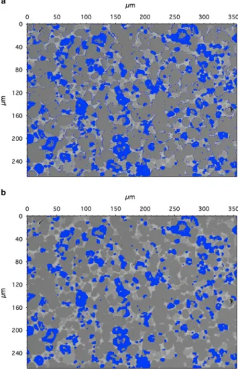
The effect of applying the bulk erosion to thefinal pixel assignment can be envisaged on Figures 5a and 5b, where eroded pixels on the latter figure, i.e. pixels discarded for creating cumulative phase spectra, are blacked out. Note, that the number of remaining pixels used for the spectra for e.g. the silicate liquid (Fig. 5c) is significantly reduced, but the resulting spectrum is considered to be free of mixed pixels. Morphology Operations on Individual Groups

Erosion, combined with complementary dilation (an algorithm that adds pixels), form the basis of standard binary image processing algorithms, the so-called “Opening” (erosion followed by dilation) and “Closing” (dilation followed by erosion) operations (e.g., Dougtherty, 1992). Combinations of Figure 4. a: Density plot of the principle component maps (PCMs) associated with the largest variances across all elemental maps. Such a representation provides an objective way of visualiz-ing populations with distinct chemical features. Pixels in the yellow region of interest (ROI) are back-traced for pixel segmenta-tion (see text). For computasegmenta-tional convenience PCMs are scaled to values from 0–255. b: Similar representation as above but displaying each individual pixel in its group color (see Figure 3). This shows that the orange group hosts two chemical features that need to be separated using ROI tools.

erosion and dilation (and opening and closing) can be applied to single groups of pixels to refine a groups’ morphology. An application is shown in Figure 6. The pixel assignment of the blue group (ortho-pyroxene) is based purely on the automated, threshold-based algorithm followed by auto-merging as described above. The assignment clearly covers larger grains, but also produces artifacts around other phases, due to effects of overlapping excitation volumes. When forming cumulative phase spectra, such pixels would be eliminated by the bulk erosion method, thus, to obtain the chemical composition of this phase, no further action is required. However, if the

purpose is to further investigate e.g. the grain size distribution of this phase on a binary image, such artifacts would clearly introduce a systematic error. Applying an opening operation results in a much cleaner and, based on morphological con-siderations, much more plausible phase assignment, which also should give a more accurate value for the modal abundance of this phase. Closing operations can be useful if larger grains of a phase exist in which single pixels, due to insufficient counting statistics, are incorrectly associated with other groups. When activating the standard bulk erosionfilter, the missing pixels would cause large proportions of the bigger grains to be elimi-nated, thus reducing the amount of pixels in eroded, cumulative spectra significantly. For smaller particles, missing pixels within such objects may actually cause complete elimination of a phase after erosion. This can be avoided if appropriate morphology operations are applied.

iSpectra Output

iSpectra’s output consists of cumulative phase spectra saved in industry standard EMSA format (Egerton et al., 1991) for Figure 5. Final pixel assignment before (a) and after applying

erosion to all groups. Eroded pixels, i.e. pixels discarded for form-ing cumulative phase spectra are blacked out (b). (c) Note that erosion significantly reduces the number of pixels used to form cumulative spectra as it can be seen in the columns“EDS Pixels” versus“Pixels” on the iSpectra group panel.

Figure 6. Combinations of standard binary erosion and dilation operations can be applied to individual groups of pixels to refine the morphology of a phase. (a) Before and (b) after applying an opening operation to one group of pixels. The result (b) is, based on morpho-logical considerations, a far more plausible phase assignment.

standardless quantification in conventional EDS software packages. Phase maps before and after binary erosion, PCM- and RGB-images are exported as TIFF images. The modal proportions of the phases as area percent and the color assignment are saved in addition. An HTML summary file, to be opened with a standard internet browser, is created on data export for easy reviewing of the entire graphical output. This is also useful for printing or converting the results into a single PDF document.

Phase maps with consistent appearance in terms of colors of phases from various data sets can be generated by using the built-in tools to create or apply a color data base in which given phase names are linked tofixed 16-bit RGB colors.

A

PPLICATIONS

Batch Processing and Large-Scale Phase Maps

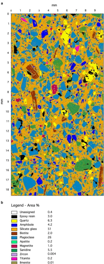
iSpectra is written such that every operation that changes pixel assignments can be formulated as simple IGOR command or as a sequence of commands to call user-defined functions, which, when recorded and subsequently executed, allow thefinal appearance of the phase map to be exactly reproduced. The record of these commands, a“history” text wave, can be used just for saving the results but can also be applied to any other SI that is expected to contain the same phases if it was recorded under identical acquisition properties. This is typically the case when mapping larger areas of one sample in automated SI grid acquisition.

An application of batch processing with the purpose of building a large phase map is shown in Figure 7. The sample is a petrographic thin section of a volcanic rock from the Fish Canyon Tuff of the Southern Rocky Mountain Volcanic Field, Colorado (for background information, see Bachmann et al., 2002 and Lipman & Bachmann, 2015). The resulting total phase map (true dimensions of 10 × 19 mm) is assembled from 4 × 10 individual SI acquired in grid mode on a Thermo Scientific NORAN System 7 X-ray microanalysis system equipped with a 30 mm2 SSD detector. The acquisition took place on a JEOL JSM-6390 LA scanning electron microscope with an LaB6filament at 15 kV and a beam current of 7.5 nA. Each SI has a dimension of 256 × 192 pixels with 2,048 channels. At a magnification of 50 × this results in a pixel or step size of 9.7µm. The acquisition time was 25 min per SI or 17 h in total, which resulted in about 2,000 average counts for each individual pixel spectrum. The original SI data sets were converted to Lispix format using the conversion program “SIconvert.exe” from Thermo Scientific. The resulting pixel spectra are fully dead-time corrected.

Pixel-to-phase assignment was carried outfirst in detail on one SI and subsequently tested and modified on other SIs by adding previously unseen phases to the historyfile before starting batch processing on the entire data set. Most of the phases are assigned purely on the basis of elemental budgets (see modal phase proportions and standardlessly derived chemical compositions in Table 1) and some merging operations to reduce the number of ghost-groups. For

Figure 7. a: Large phase map (10 × 19 mm) of a volcanic rock assembled from batch processing 40 (4 × 10) individual SIs acquired in an overnight automated grid measurement. b: Phase legend including area percentages.

example, apatite is recognized by the presence of Ca and P, FeOx (magnetite) by presence of Fe and titanite by Si, Ca, and Ti (all defined by Kα energies). Biotite is defined by the simultaneous presence of Mg, Al, Si, and K, but is refined by applying a closing morphology operation in order to minimize the occurrence of ghost-groups within larger biotite grains. Plagioclase and K-feldspar are separated from the other major silicate phases on the basis of density plots and distinct populations in Na versus Si and K versus Si space, respectively. The matrix is a devitrified former glass and consists to a large extent of intergrowths of small Al-rich silicate and small K-Feldspar crystals. The sizes of such grains are generally smaller than the step size in these maps, which is why the matrix appears largely homogeneous. However, the presence of K-Feldspar crystals as large phenocrysts and as part of the matrix makes a clear separation between both phases difficult. This can be seen by the presence of pixels of these phases inside each other. Applying a morphology operation to the K-feldspar group pixels would improve the assignment covering the phenocrysts but would leave clearly visible artifacts inside the matrix. Groups of pixels that are not defined as phases, i.e. they were not given a phase name, were automatically merged into a group of unassigned pixels (trash) during batch processing if their area percentage was<0.15% (which can be set as a user-defined threshold). Groups of unuser-defined pixels larger than this threshold were analyzed by the particle analysis operation if such pixels occured as a group of contiguous, i.e. connected pixels. If yes, this group had been marked as“unknown phase”; if not, such pixels were merged with“trash.” In the present case, the total amount of unassigned pixels is just 0.4%.

Batch processing produces the following output per SI: a phase map and its eroded version, the main PCM, optionally an RGB image and the cumulative phase spectra after bulk erosion. Average chemical compositions from such spectra were subsequently quantified in NSS and are reported in Table 1. The individual images can be loaded and assembled as one large image including overlap correction as presented in Figure 7a. Batch processing produces two text files; one summarizing the phases (including unassigned pixels), their elemental budgets, total number of pixels per groups, the pixels

percentage, and the number of pixels after erosion for further data processing. A“phase legend,” which is complementary to the large phase map and showing the color for each phase and its area percentage (Fig. 7b), can automatically be generated from this textfile. The second text file is a log-file that reports details on the batch processing, e.g. in case additional “unknown phases,” as described in the previous section, are detected. The log-file can then be used for inspection purposes and to specifically change the pixel assignment in the history file for an improved batch output.

Inclusion Analysis

By default, iSpectra creates cumulative EDS spectra of all pixels associated with one group either on export or for spectrum review during pixel-to-phase assignment. How-ever, it can be desirable to compare spectra and thus che-mical compositions of different particles of one group. The “single phase analysis” option implemented in iSpectra supports export of EDS spectra of individual particles of one group including their image coordinates, particle sizes, and shape parameters, e.g. circularity.

Figure 8a shows a grain of Haüyne [a tectosilicate with an ideal composition of Na3Ca(Si3Al3)O12(SO4); see Cooper, et al. (2015) for background information], which hosts a number of melt inclusions. The aim of this investigation was to study the variability in chemical composition of such inclusions. For this purpose, a traverse over the core of the grain was measured in four consecutive SIs (see Fig. 8a). The instrument was the same as described above and the acqui-sition was carried out at a magnification of 1,200 × and an SI resolution of 512 × 384 pixels resulting in a step size of 0.2µm. The total acquisition time on one SI was 210 min with counts on each pixel spectrum on the order of 2,200. The phase segmentation between the Haüyne matrix and the melt inclusions was done using an Si versus Al elemental density plot. To minimize the effect of mixed pixels a 5 × 5 circular structure element was applied for erosion. This resulted in a width of eroded pixels between inclusions and the matrix of typically 6–7 pixels or 1.2–1.4 µm, which is

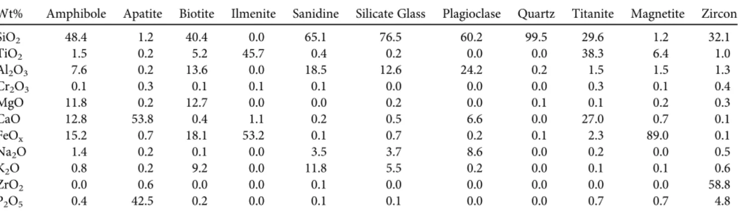
Table 1. Average Chemical Compositions from 40 Individual Spectral Images Derived from Cumulative Phase Spectra Generated During Batch Processing (After Erosion Was Being Applied).

Wt% Amphibole Apatite Biotite Ilmenite Sanidine Silicate Glass Plagioclase Quartz Titanite Magnetite Zircon

SiO2 48.4 1.2 40.4 0.0 65.1 76.5 60.2 99.5 29.6 1.2 32.1 TiO2 1.5 0.2 5.2 45.7 0.4 0.2 0.0 0.0 38.3 6.4 1.0 Al2O3 7.6 0.2 13.6 0.0 18.5 12.6 24.2 0.2 1.5 1.5 1.3 Cr2O3 0.1 0.3 0.1 0.1 0.1 0.0 0.0 0.0 0.3 0.1 0.4 MgO 11.8 0.2 12.7 0.0 0.0 0.2 0.0 0.1 0.1 0.2 0.3 CaO 12.8 53.8 0.4 1.1 0.2 0.5 6.6 0.0 27.0 0.7 0.1 FeOx 15.2 0.7 18.1 53.2 0.1 0.7 0.2 0.1 2.3 89.0 0.1 Na2O 1.4 0.2 0.1 0.0 3.5 3.7 8.6 0.0 0.2 0.0 0.5 K2O 0.8 0.2 9.2 0.0 11.8 5.5 0.2 0.0 0.1 0.1 0.6 ZrO2 0.0 0.6 0.0 0.0 0.1 0.0 0.0 0.0 0.0 0.0 58.8 P2O5 0.4 42.5 0.2 0.0 0.1 0.1 0.0 0.0 0.7 0.7 4.8

equivalent to the size scale of the expected excitation volume, thus increasing the likelihood that only true inclusion compositions are considered (Fig. 8b). Only inclusions with more than 10 pixels were exported, which resulted in 171

individual spectra across the four SIs. The 10 pixel threshold considers that at least a minimum number of total counts is required for reliable spectrum quantification. Standardless quantification was carried out in the NSS 7. The results as Figure 8. a: Back-scattered electron image of an inclusion bearing Haüyne crystal from Tenerife. The blue rectangle indicates the area, which was covered with four spectral images (SIs) to determine the melt inclusion compositions along a traverse though the grain. b: Result of the phase segmentation on e.g. a Si versus Al density plot on one SI. The influence of mixed pixels in each individual inclusion was minimized by using a 5 × 5 circular structure element for bulk erosion. c: Inclusion map composition in terms of wt% Al2O3after spectrum evaluation.

weight percent oxides per inclusion were then copied to IGOR and iSpectra, where the actual wt% values for a given element were then “seed-filled” to each corresponding inclusion on a binary mask. The graphical outcome, after assembling results for the four different SIs, is an inclusion map (Fig. 8c), which shows color coded the chemical compositions of the inclusion over the entire traverse (here for weight percent Al2O3), which provides an excellent way for visualizing chemical variability in such systems.

D

ISCUSSION

As demonstrated in the previous sections, iSpectra is a powerful toolbox for the analysis of SIs with a variety of possible applications. Because iSpectra is system independent, i.e. it can be used to analyze data sets acquired on different EDS systems, it is well suited to extend the functionality of EDS software packages in many SEM laboratories. However, certain limita-tions in the applicability of iSpectra should be considered.

As explained above, iSpectra works with specific element lists, which implies that elements are not recognized if peak energies are not defined. Although iSpectra provides a tool to identify unspecified energies (the Bright & Newbury, 2004 “maximum pixel spectrum”) it still remains the responsibility of the analyst to arrange an appropriate list. iSpectra allows loading of different lists of elements and their corresponding energies, thus the user may import, depending on the nature of the specimen, specific sets of elements that are best suited for the present sample. However, working with iSpectra generally requires some foreknowledge on the sample chemistry.

A related problem is that iSpectra does not perform peak fitting and thus, does not deconvolute overlapping peaks, which may cause severe problems in separating phases containing elements with overlapping energies. Note that identifying overlapping peaks is, under some circumstances, nontrivial as pointed out by Newbury (2005, 2007), and is outside the scope of this toolbox. On the other hand, peak overlap is not necessarily a major obstacle for pixel-to-phase assignments: the phase map in Figure 7 contains two phases where two elements show peak overlap; Ca5(PO4)3apatite and with PK-α1 at 2.02 keV and ZrSiO4 zircon with ZrL-α1 at 2.04 keV. Both, the elemental maps of P and Zr will show high intensity where either of these two minerals are present, but the unique combination of the overlapping elements with Si or Ca, respectively, makes phase segmentation possible. This however, requires a certain level of understanding of the possible phase chemistry in the system of interest and may lead to misinterpretation by inexperienced users.

iSpectra should therefore rather be considered as a tool for intermediate to advanced analysts with knowledge of the caveats in energy-dispersive analysis (e.g., such as overlap problems) and with a solid level of understanding in the phase chemistry of the investigated materials. However, iSpectra will allow such usersfine control over the pixel-to-phase assign-ments down to every single pixel, which is usually not achievable on commercial phase mapping products. The pre-sent limitations in iSpectra also imply that the analysis and

pixel-to-phase assignment of certain materials is expected to be more successful compared with others. Analysis of geological materials, as shown in this paper, results in very good and plausible results. This is the case because emission energies of major and minor elements generally show little overlap, such that peaks are mostly clearly separable, which is key for reliable phase mapping. The default list of elements implemented in iSpectra is suited for this kind of material, as this is the authors primaryfield of interest. However, the situation may be dif-ferent when working on e.g. inter-metallic alloys or semi-conductor materials including heavy elements such as e.g. different lanthanides with potentially severe overlap of L- or M-emission lines. However, iSpectra will be continuously developed and improved and its open source nature may eventually lead to contributions that will help to overcome some of the limitations above.

S

UMMARY AND

C

ONCLUSIONS

iSpectra is a powerful open source and system-independent toolbox for the analysis of SIs that can be used in addition to many commercial EDS analysis software packages for extended and individualized functionality. The approach to assigning pixels to phases is similar to some techniques presented in the PARC method by van Hoek et al. (2011) and van Hoek (2014), but is extended by the ability of applying a variety of fundamental binary image analysis tools, such as image morphology or particle analysis operations, to groups of pixels. This spectral imaging toolbox does require a priori knowledge of the sample material but offers advanced users with a solid understanding of EDS analysis and phase chemistry very detailed control over the pixel-to-phase assignments to create chemically and texturally plausible phase maps.

A

CKNOWLEDGMENTS

The author is grateful to Corrie van Hoek and Sieger van der Laan from the Ceramic Research Centre (CRC) of TATA Steel Europe RD&T (IJmuiden, The Netherlands) for having the opportunity to work with the PARC method during my time at CRC. This has clearly influenced the development of iSpectra. The author would like to thank Daniel Weidendorfer and Eric Reusser for discussions as well as Lauren Cooper for providing the Hayüne example and Olivier Bachmann for the Masonic Park tuff sample. The author thanks Amir Khan for his comments on PCA and acknowledges the comments of three anonymous reviewers, whose constructive criticism significantly improved the manuscript.

R

EFERENCES

BACHMANN, O., DUNGAN, M.A. & LIPMAN, P.W. (2002). The Fish

Canyon magma body, San Juan volcanic field, Colorado: Rejuvenation and eruption of an upper-crustal batholith. Journal of Petrology 43, 1469–1503.

BONNET, N., SIMOVA, E., LEBONVALLET, S. & KAPLAN, H. (1992). New applications of multivariate statistical analysis in spectroscopy and microscopy. Ultramicroscopy 40, 1–11.

BRIGHT, D.S. (1987). A LISP-based image analysis system with

applications to microscopy. J Microsc 148, 51–87.

BRIGHT, D.S. & NEWBURY, D.E. (1991). Concentration histogram

imaging—A scatter diagram technique for viewing 2 or 3 related images. Anal Chem 63, A243–A250.

BRIGHT, D.S. & NEWBURY, D.E. (2004). Maximum pixel spectrum: A

new tool for detecting and recovering rare, unanticipated features from spectrum imaging cubes. J Microsc 216, 186–196. COOPER, L.B., BACHMANN, O. & HUBER, C. (2015). Volatile budgets of

volcanoes inferred from textural zonation of S-rich haüyne. Geology 43, 423–426.

DOUGTHERTY, E.R. (1992). Mathematical Morphology in Image

Processing. New York: CRC Press.

DROUIN, D., COUTURE, A.R., JOLY, D., TASTET, X., AIMEZ, V. & GAUVIN, R. (2007). CASINO V2.42—A fast and easy-to-use modeling tool for scanning electron microscopy and microanalysis users. Scanning 29, 92–101.

EGERTON, R.F., FIORI, C.E., HUNT, J.A., ISAACSON, M.S., KIRKLAND, E.J.

& ZALUZEC, N.J. (1991). EMSA/MAS standard file format for

spectral data exchange. EMSA Bull 21, 35–41.

FRIEL, J.J. & LYMAN, C.E. (2006). X-ray mapping in electron-beam instruments. Microsc Microanal 12, 2–25.

KOTULA, P.G., KEENAN, M.R. & MICHAEL, J.R. (2003). Automated analysis of SEM X-ray spectral images: A powerful new microanalysis tool. Microsc Microanal 9, 1–17.

LANARI, P., VIDAL, O., DE ANDRADE, V., DUBACQ, B., LEWIN, E.,

GROSCH, E.G. & SCHWARTZ, S. (2014). XMapTools: A MATLAB

(c)-based program for electron microprobe X-ray image processing and geothermobarometry. Comput Geosci 62, 227–240.

LIPMAN, P.W. & BACHMANN, O. (2015). Ignimbrites to batholiths: Integrating perspectives from geological, geophysical, and geochronological data. Geosphere 11, 705–743.

LUCAS, G., BURDET, P., CANTONI, M. & HEBERT, C. (2013). Multivariate

statistical analysis as a tool for the segmentation of 3D spectral data. Micron 52–53, 49–56.

MALOY, A.K. & TREIMAN, A.H. (2007). Evaluation of image classification routines for determining modal mineralogy of rocks from X-ray maps. Am Mineral 92, 1781–1788.

NEWBURY, D.E. (2005). Mistakes encountered during automatic

peak identification in low beam energy x-ray microanalysis. Scanning 29, 137–151.

NEWBURY, D.E. (2007). Misidentification of major constituents

by automatic qualitative energy dispersive x-ray microanalysis: A problem that threatens the credibility of the analytical community. Microsc Microanal 11, 545–561.

MALOY, A.K. & TREIMAN, A.H. (2007). Evaluation of

image classification routines for determining modal mineralogy of rocks from X-ray maps. Am Mineral 92, 1781–1788.

PARISH, C.M. (2011). Multivariate statistics applications in scanning

transmission electron microscopy X-ray spectrum imaging. In Advances in Imaging and Electron Physics, Hawkes, P.W. (ed.), pp. 249–295.

PRET, D., SAMMARTINO, S., BEAUFORT, D., MEUNIER, A., FIALIN, M. &

MICHOT, L.J. (2010). A new method for quantitative petrography

based on image processing of chemical element maps: Part I. Mineral mapping applied to compacted bentonites. Am Mineral 95, 1379–1388.

SCHAMBER, F.H. (1977). A modification of the least-squares fitting

method which provides continuum suppresion. In X-ray Analysis of Environmental Samples, Dzubay, T.G. (ed.), pp. 241–257). Ann Arbor, MI: Ann Arbor Science Publishers.

STATHAM, P.J. (1977). Deconvolution and background subtraction

by least-squaresfitting with prefiltering of spectra. Anal Chem 49, 2149–2154.

VAN HOEK, C. (2014). How to process zillions of spectra from

spectral imaging datasets? From phase mapping to bulk-chemistry on micron- to centimeter scale using PARC. Microsc Microanal 20(S3), 660–661.

VANHOEK, C.J.G.,DEROO, M.,VAN DERVEER, G. &VAN DERLAAN, S.R.

(2011). A SEM-EDS study of cultural heritage objects with interpretation of constituents and their distribution using PARC data analysis. Microsc Microanal 17, 656–660.