HAL Id: tel-03166430
https://tel.archives-ouvertes.fr/tel-03166430
Submitted on 11 Mar 2021HAL is a multi-disciplinary open access archive for the deposit and dissemination of sci-entific research documents, whether they are pub-lished or not. The documents may come from teaching and research institutions in France or abroad, or from public or private research centers.
L’archive ouverte pluridisciplinaire HAL, est destinée au dépôt et à la diffusion de documents scientifiques de niveau recherche, publiés ou non, émanant des établissements d’enseignement et de recherche français ou étrangers, des laboratoires publics ou privés.
Non-Local Modeling of the Compressive Strength of
Composite Structures
Anil Bettadahalli Channakeshava
To cite this version:
Anil Bettadahalli Channakeshava. Non-Local Modeling of the Compressive Strength of Composite Structures. Other. ISAEENSMA Ecole Nationale Supérieure de Mécanique et d’Aérotechique -Poitiers, 2020. English. �NNT : 2020ESMA0018�. �tel-03166430�
THESE
Pour l’obtention du Grade de
DOCTEUR DE L’ECOLE NATIONALE SUPERIEURE DE MECANIQUE ET
D’AEROTECHNIQUE
(Diplôme National – Arrêté du 25 mai 2016) Ecole Doctorale :
Sciences et Ingénierie en Matériaux, Mécanique, Energétique et Aéronautique Secteur de Recherche : Mécanique des solides, des Matériaux, des Structures et des Surfaces
Présentée par :
Anil BETTADAHALLI CHANNAKESHAVA ****************************
MODELISATION NON-LOCALE DE LA RESISTANCE EN COMPRESSION DES COMPOSITES ARCHITECTURES
-
NON-LOCAL MODELING OF THE COMPRESSIVE STRENGTH OF COMPOSITE STRUCTURES ****************************
Directeur(s)de thèse : Jean-Claude GRANDIDIER ****************************
Soutenue le 17th Décembre 2020 devant la Commission d’Examen
****************************
JURY
Président :
DRAPIER Sylvain, Professeur, Ecole des Mines de Saint-Etienne, Saint-Etienne Rapporteurs :
PIMENTA Soraia, Senior lecturer, Imperial College London (UK)
GANGHOFFER Jean- François, Professeur, Université de Lorraine, Lorraine Membres du jury :
DRAPIER Sylvain, Professeur, Ecole des Mines de Saint-Etienne, Saint-Etienne KERYVIN Vincent, Professeur, Université Bretagne Sud, Lorient
MECHIN Pierre-Yves, Directeur de Recherche, Dassault Systèmes GRANDIDIER Jean-Claude, Professeur, ISAE-ENSMA, Poitiers
A
CKNOWLEDGEMENTS
First and foremost, I would like to express my sincere gratitude to Prof. Jean-Claude GRANDIDIER for giving me this PhD opportunity with Institute Pprime/ISAE-ENSMA and his immense support, encouragement, patience and motivation throughout my thesis. His vast experience in the field of finite elements brings lots of insight to my computational knowledge. It was really a great pleasure to work under him. Also, I would like to thank all my friends and other colleagues in the laboratory who contributed to the success of finishing my thesis.
A special thanks to my parents, my brother and my beloved wife Anusha for their love and support continuously throughout my thesis. Without their motivation and support it would not be possible for me to complete my work.
A
BSTRACT
The compressive failure of long carbon fiber composites is due to complex mechanisms. The knowledge of these mechanisms is important for the design of composite structures because the compressive strength and stiffness of laminates are assumed less than their tensile strength. Further, compressive failure is a mechanism of non-local ruin that depends on the composite structure (layer thickness, load gradient) which makes it a peculiarity. The mechanism has been described and modelled in the literature with suitable numerical tools and experiments that accounted for this effect. There are many articles in the literature regarding the modelling of composites compressive behavior, particularly the microbuckling phenomenon / local instability. But only a few researchers modelled the mechanism at the structural/mesoscopic scale. For example, Drapier et al., [D3] proposed a 2D homogenized model, which takes into account fiber initial alignment defects, matrix plasticity and structural parameters. The model is successful in predicting the elastic microbuckling modes and to predict the failure. But the model is built for 2D unidirectional laminates and assumes microbuckling is periodic in the fiber direction, just one gradient in the thickness direction is taken into account and the influence of the misalignment is not completely described [D4]. Therefore, to extend the developments of these works ([D1],[D3],[G1],[G4]), new non-local finite element models are developed: one with using ABAQUS® in-built structural elements, named Beam Non-Local (BNL) model and the other with User Element (UEL) subroutine of ABAQUS®, named Homogenized Non-Local Model (HOMNL), implemented in the user element (NL U32), which can be applied with the aim to predict the compressive strength of unidirectional plies/laminates and also for woven composites (2D and 3D). Both the non-linear geometrical and material effects are taken into account in this model. With the BNL model, it is possible to capture the mechanism in 2D and 3D space for laminates of unidirectional composites. Results of the bibliography have been confirmed and new results are presented, for example, the elastic mode in 3D or the mechanism under bending. The width and angle of the kink band are determined by this model. In the framework of more general, the validation of the NL U32 element has been performed with respect to ABAQUS® classical elements for both linear and non-linear (geometry and material) cases. The classical (elastic and plastic) and non-local material properties (elastic) are identified by comparison to the responses of a Representative Volume Element (RVE) of full heterogenous microstructures. Some results have been validated with the bibliography. The developed non-local user element (NL U32) is 2D in this thesis and it can be extended easily to a 3D case, which remains one of the future perspectives.
In this work, ABAQUS® v2017, DAKOTA v6.10.0, PARAVIEW v5.8.0 are the softwares used and FORTRAN, Python are the programming languages used.
Keywords : Compressive strength, Long carbon fiber composites, Non-Local model, Finite
R
ÉSUMÉ
La rupture en compression des composites à fibers de carbone longues est due à des mécanismes complexes. La connaissance de ces mécanismes est importante pour la conception des structures composites car la résistance à la compression et la rigidité des stratifiés sont supposées inférieures à leur résistance à la traction. De plus, la rupture en compression est un mécanisme de ruine non locale qui dépend de la structure du composite (épaisseur de la couche, gradient de charge), ce qui en fait une particularité. Ce mécanisme a été décrit et modélisé dans la littérature avec des outils numériques appropriés et des expériences qui ont pris en compte cet effet. Il existe de nombreux articles dans la littérature intégrant le phénomène de microflambage pour capter l’instabilité locale. Mais uniquement quelques chercheurs ont modélisé le mécanisme à l'échelle structurelle dite mesoscopique. Par exemple, Drapier et collaborateurs ont proposé un modèle homogénéisé en 2D, qui prend en compte les défauts d'alignement initial des fibers, la plasticité de la matrice et les paramètres structurels. Le modèle permet de prédire les modes de microflambage élastique et de prévoir la défaillance en compression. Mais le modèle est construit pour des stratifiés unidirectionnels 2D et suppose que le microflambage est périodique dans la direction des fibers, un seul gradient dans la direction de l'épaisseur est pris en compte et l'influence du désalignement n'est pas complètement appréhendée.Par conséquent, pour étendre les développements de ces travaux, de nouveaux modèles d'éléments finis non locaux sont développés dans cette thèse : l'un avec des éléments de structures proposés de base par ABAQUS®, appelé modèle BNL (Beam Non-Local) et l'autre avec le sous-programme UEL (User Element) d'ABAQUS®, appelé modèle HOMNL (Homogenized Non-Local Model), mis en œuvre sous la forme d’un élément utilisateur (NL U32), qui peut être utilisé dans le but de prédire la résistance à la compression des plis stratifiés unidirectionnels mais également pour les composites tissés (2D voire 3D). Les effets de non linéarités géométriques et matériels sont bien évidemment pris en compte dans cette modélisation. Avec le modèle BNL, il est possible d’appréhender le mécanisme en 2D et 3D dans des stratifiés de composites unidirectionnels. Les résultats de la bibliographie ont été confirmés et de nouveaux résultats ont été générés, comme par exemple, le mode élastique en 3D ou le mécanisme de microflambage en flexion dans un stratifié. La largeur et l'angle de la bande de pliage sont déterminés automatiquement par ce modèle. Dans un cadre plus général, la validation de l'élément NL U32 a été effectuée par rapport aux éléments classiques ABAQUS® pour les cas linéaires et non linéaires (géométrie et matériau). Les propriétés classiques (élastiques et plastiques) et non locales des matériaux (élastiques) sont identifiées par comparaison avec les réponses d'un élément de volume représentatif (RVE) de microstructures totalement hétérogènes. Certains résultats de résistances ont été validés avec la bibliographie. L'élément utilisateur non local développé (NL U32) est en 2D dans cette thèse mais il peut être étendu très facilement à un cas en 3D, ce qui reste une des perspectives futures.
Dans ce travail, ABAQUS® v2017, DAKOTA v6.10.0, PARAVIEW v5.8.0 sont les logiciels utilisés et FORTRAN, Python sont les langages de programmation.
Mots-clés : Résistance en compression, Composites à fibers longues, modèle non local, élément
Table of Contents
ACKNOWLEDGEMENTS ... 3 ABSTRACT ... 5 RÉSUMÉ ... 6 LIST OF FIGURES ... 11 LIST OF TABLES ... 17 1 Introduction ... 19 2 About Composites ... 21 2.1 Classification of composites ... 222.1.1 First Level (Matrix Material) ... 22
2.1.2 Second Level (Reinforcement form) ... 22
2.2 Laminated Composites... 22
2.3 Woven composites ... 23
2.3.1 2D Woven fabrics ... 24
2.3.2 3D Woven fabrics ... 25
2.3.3 3D woven production techniques ... 26
2.4 Defects from process/manufacturing techniques ... 29
2.5 Specific case: long carbon fiber reinforced composites ... 29
2.6 Behavior of composite materials ... 30
2.6.1 General behavior ... 30
2.6.2 Unidirectional case ... 32
2.6.3 Woven case ... 33
2.6.4 Specific problem of compression ... 33
3 Strength of composite materials under compression (experiments and models) ... 35
3.1 Compression tests ... 35
3.2 Four Point Flexion Compression Fixture ... 36
3.3 Strength of long fiber UD composites ... 37
3.4 Strength of Woven composites ... 38
3.5 Models for compression of composite materials – Theoretical Background ... 42
3.5.1 Microbuckling models for unidirectional composite ... 42
3.5.2 Modelling of woven composite in compression ... 49
3.5.3 Discussion ... 51
4 Scope of work and outline ... 53
4.1 Work package/Outline ... 54
5.1 Introduction ... 55
5.2 Beam Non-Local Model: Building the model... 56
5.2.1 Definition of properties ... 56
5.2.2 2D Validation of stiffness in elastic ... 61
5.2.3 Effect of number of beams ... 62
5.2.4 Effect of the length of ply ... 64
5.2.5 Structural effect on elastic mode – comparison with bibliography ... 65
5.2.6 Other structural effects ... 68
5.2.7 3D microbuckling ... 70
5.2.8 Material nonlinearity effect and initial defects ... 72
5.3 Conclusion ... 81
6 Generalized Non-Local model for UD and Woven composites – numerical model (UEL Abaqus®) ... 83
6.1 Introduction ... 83
6.1.1 Various Non-Local (NL) models and NL Finite Element approaches which permits to modelize compression behavior ... 83
6.1.2 Non-local Finite Element Approaches using continuum non-local models ... 89
6.2 Theoretical part ... 90
6.2.1 Principle of virtual work and equilibrium equations (2D) ... 92
6.3 Numerical development ... 94
6.3.1 Formulation of new element (for 2D UD ply and woven case) ... 94
6.3.2 FE Formulation of Non-local model implemented in NL U32 ... 98
7 Validation of NL U32 Element (Linear case) ... 113
7.1 Linear Geometry and Linear Isotropic Elastic Case ... 113
7.1.1 Case1: Compression ... 113
7.1.2 Case2: Bending ... 115
7.1.3 Discussion ... 117
7.1.4 Mesh Convergence study ... 118
7.1.5 Comparison with 2D heterogenous complete microstructure ... 118
8 Geometrical Non-Linearity in NL U32: description and validation ... 123
8.1 Formulation and addition of Geometrical Non-Linearity ... 123
8.2 Validation of Geometrical Non-Linearity ... 127
8.2.1 Case1: Compression ... 127
8.2.2 Case2: Bending ... 129
9 Matrix Material Non-Linearity in NL U32: description of the law and validation ... 131
9.1 Formulation and addition of matrix material non-linearity (Isotropic) ... 131
9.2.1 Validation of UMAT (RO Law) with CPS4 ... 134
9.2.2 Validation of matrix material non-linearity (RO Law) in NL U32 ... 136
9.2.3 Comparison with 2D heterogenous complete microstructure (Non-linear Matrix material and Non-linear geometry) ... 136
9.2.4 Anisotropic Ramberg-Osgood (RO) Law (2D Plane stress) - unidirectional composite .... 148
9.2.5 Validation of Anisotropic Ramberg-Osgood (RO) Law ... 152
10 Identification of Parameters ... 155
10.1 Identification of Elastic and Non-Local parameters ... 155
10.1.1 A brief description about DAKOTA ... 155
10.1.2 Strategy/Protocol to identify parameters ... 157
10.2 Identification of Non-Linear material parameters ... 172
10.2.1 Influence of 𝛼12 parameter ... 172
10.2.2 Identification of parameters ... 172
11 Compressive Response of Non-Local composites ... 179
11.1 Unidirectional case ... 179
11.1.1 Comparison with BNL model: Effect of thickness of ply ... 179
11.1.2 Comparison with heterogenous model ... 180
11.2 Woven case ... 181
12 Conclusion and Perspectives ... 185
13 APPENDIX ... 187
13.1 Principle of virtual work and equilibrium equations (2D)... 187
13.2 2D Plane Stress User Element (U4) ... 194
13.2.1 Abaqus UEL implementation ... 194
13.2.2 Formulation of element U4 ... 196
13.2.3 Comparison of UEL (U4) with ABAQUS® CPS4 ... 202
13.3 Derivatives of shape functions ... 206
13.3.1 Bilinear shape functions ... 206
13.3.2 Biquadratic shape functions ... 206
13.3.3 Bicubic shape functions (Hermit type) ... 207
13.4 Why order of Cf Parameters should be higher than 103? ... 213
13.5 Validation of RO laws ... 215
References ... 237
LIST OF FIGURES
Figure 1: Applications of composite materials. [D7],[B21] ... 21
Figure 2: Architecture of composite materials. ... 21
Figure 3: Long carbon fiber composite UD ply (left) and laminate (right). [B5] ... 23
Figure 4: Woven Composites and its parts (2D and 3D). [D8],[B22] ... 24
Figure 5: Types of 2D woven fabrics and its configuration. Ref: Textile Reinforced structural composites for advanced applications, [Chap 4, Karaduman, (2017)] ... 25
Figure 6: Illustration of 2D weaving principle for 2D fabrics. [Fredrik et al., (2009)] ... 25
Figure 7: Types of 3D woven composites: (a) orthogonal, (b) through the thickness angle interlock, (c) layer-to-layer angle interlock, and (d) fully interlaced (plain 3D weave). [Fredrik et al., (2009)] ... 26
Figure 8: Illustration of 2D weaving principle for 3D fabrics. [Fredrik et al., (2009)] ... 27
Figure 9: Schematic representation of warp and weft yarns with a crossover of binder yarn in 3D woven fabrics (orthogonal). [Elsaid et al., (2014)] ... 27
Figure 10: Illustration of 3D weaving principle for 3D fabrics, seen from the warp or 1-direction. [Fredrik et al., (2009)] ... 28
Figure 11: A plain 3D-weave without stuffer yarns seen from its three principle planes and from an isometric view. Warp yarns are blue, horizontal weft yarns red and vertical weft yarns green in the illustrations. [Fredrik et al., (2009)] ... 28
Figure 12: UD Carbon/Epoxy (CFRP) Composite. [Thirumalai et al., (2017)] ... 30
Figure 13: Examples of Compressive failures at structural scale ... 34
Figure 14: Celanese Fixture (left) and IITRI Fixture (right). [A2] ... 35
Figure 15: Combined Loading Compression test Fixture. [A2] ... 36
Figure 16: Schematic of Flexure tests (3-point and 4-point test). [I1] ... 37
Figure 17: Initial fiber waviness. [Sun et al., (1994)] ... 37
Figure 18: Formation of kink bands (plastic microbuckling phenomenon). [Drapier et al., (1999)] ... 38
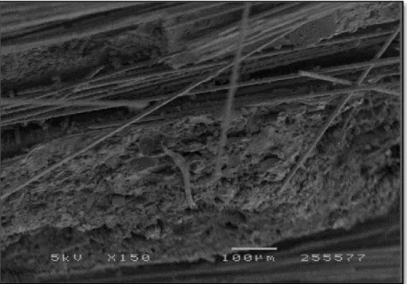
Figure 19: SEM fractograph of woven carbon fiber epoxy composite after fracture under compression (36.8% vol). [Ghafaar et al., (2006)]... 39
Figure 20: Comparison of compressive failure of cuboidal specimens of (a) lightly compacted composites, and (b) a heavily compacted composite, that failed by delaminating. [Cox et al. (1994)] ... 40
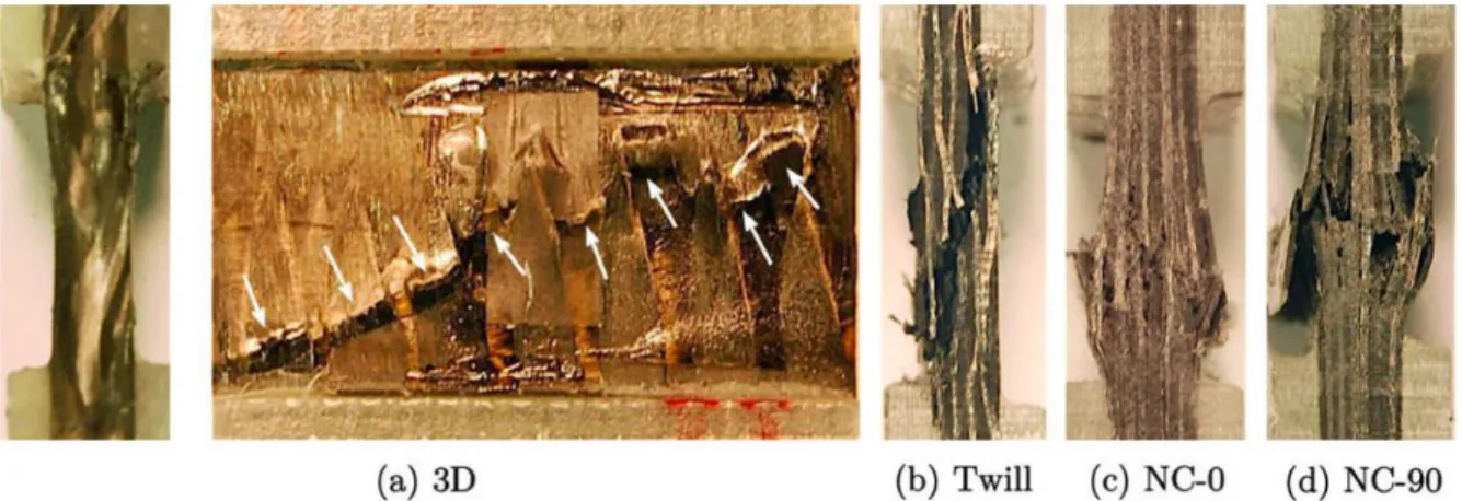
Figure 21: Failure modes in compression. (a) The warp yarns in the 3D specimens fail locally at an angle, see the right hand image, (b) fiber failure in the Twill and (c) + (d) brooming fiber failure of the two non-crimp laminates. [Fredrik et al., (2009)] ... 40
Figure 22: longitudinal compressive failure for (a) ply to ply 12 K/24 K, (b) ply to ply 24 K/24 K and (c) quasi-isotropic 2D woven fiber architectures. [Warren et al., (2015)] ... 41
Figure 23: 3D orthogonal woven carbon composites: Full TTT reinforcement (left) and Half TTT reinforcement (right). [Turner et al. (2016)] ... 42
Figure 24: Microbuckling modes. [Rosen, 1964] ... 43
Figure 25: Hierarchical levels of woven/textile-based composites. [M6] ... 50
Figure 26: Approximation of woven fabric as anisotropic continuum medium (left); fabric model geometry (right) [King et al., (2005)] ... 51
Figure 27: Comparison of global stiffness calculated with heterogenous model and non-local BNL model ... 62
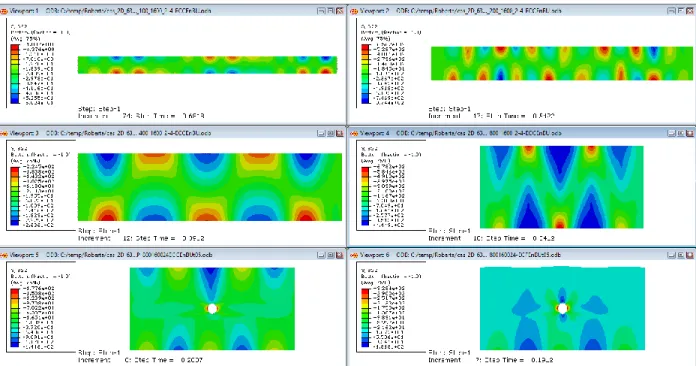
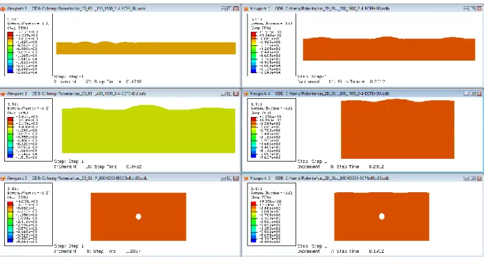
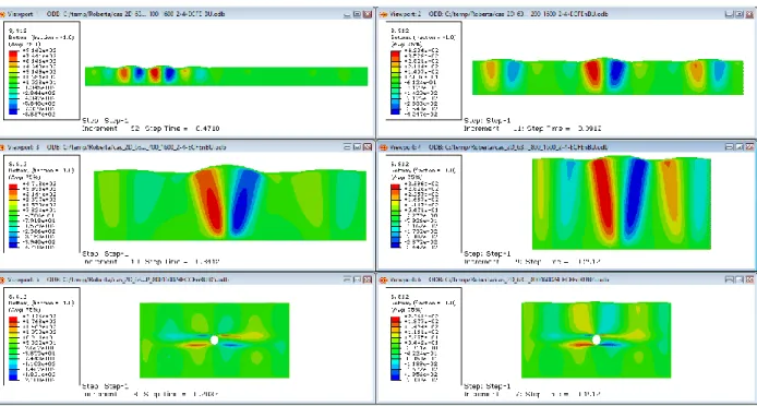
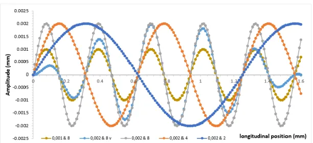
Figure 28: Influence of number of beams in 2D case (extract to internship of Roberta Maziotta) ... 63
Figure 29: Influence of number of beams in 3D case (extract to internship of Roberta Maziotta) ... 63
Figure 30: Clamped-Clamped (left) and Clamped-Free BC’s (right) ... 64
Figure 31: Critical stain in function of length of ply ... 64
Figure 32: Critical stain in function of thickness of ply... 65
Figure 34: Critical mode in function of thickness of ply (Clamped-Free BC's) ... 67
Figure 35: Comparison of modal displacements over ply thickness with Drapier et al., (1996) for clamped-clamped and clamped-clamped-free condition under pure compression ... 68
Figure 36: Elastic microbuckling mode in unidirectional ply under bending; clamped at left edge ... 69
Figure 37: Elastic microbuckling mode in [90°,0°,90°] laminate under compression; upper, lower and left edges are clamped ... 69
Figure 38: Elastic microbuckling mode in [90°,0°,90°] under bending; clamped at left edge ... 70
Figure 39: Elastic microbuckling mode in unidirectional case under compression just beams are represented in the right picture and a transverse cut is applied) ... 70
Figure 40: Elastic microbuckling mode in [90°,0°,90°] under compression; upper, lower and left faces are clamped (just beams are represented in right picture) ... 71
Figure 41: Elastic microbuckling mode in [90°,0°,90°] under bending; left face clamped (just beams in UD ply are represented in right picture) ... 71
Figure 42: Evolution of components of stiffness matrix in function of equivalent strain and comparison of nonlinear behavior under three different loads ... 73
Figure 43: Critical strain for different thickness on unidirectional ply under compression with two boundary conditions ... 74
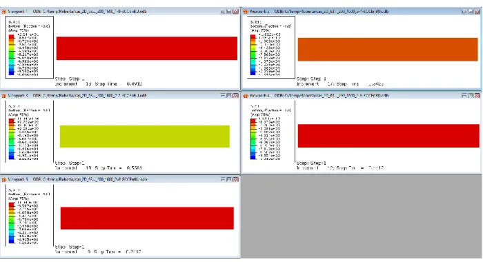
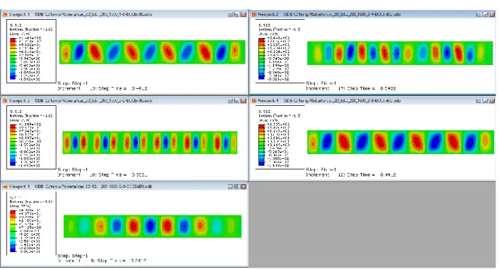
Figure 44: Fields of longitudinal stress at instability for a unidirectional ply under compression (clamped-clamped) – bottom right (clamped-free) ... 74
Figure 45: Fields of transverse stress at instability for a unidirectional ply under compression (clamped-clamped) – bottom right (clamped-free) ... 75
Figure 46: Fields of shear stress at instability for a unidirectional ply under compression (clamped-clamped) – bottom right (clamped-free) ... 75
Figure 47: Fields of longitudinal stress at instability for a unidirectional ply under compression (clamped-free) – bottom left (clamped-clamped) ... 76
Figure 48: Fields of transverse stress at instability for a unidirectional ply under compression (clamped-free) – bottom left (clamped-clamped) ... 76
Figure 49: Fields of shear stress at instability for a unidirectional ply under compression (clamped-free) – bottom left (clamped-clamped) ... 77
Figure 50: Evolution in the length of amplitude for studying defects ... 78
Figure 51: Evolution in the length of angle for studying defects ... 78
Figure 52: Critical strain in function of maximal angle ... 79
Figure 53: Critical strain in function of parameters of defect ... 79
Figure 54: Fields of longitudinal stress at instability for a unidirectional 200µm ply under compression (clamped-clamped)- definition of defect: ... 80
Figure 55: Fields of transverse stress at instability for a unidirectional 200µm ply under compression (clamped-clamped)- definition of defect: ... 80
Figure 56: Fields of shear stress at instability for a unidirectional 200µm ply under compression (clamped-clamped)- definition of defect: ... 81
Figure 57: Non-Local Super-parametric element (NL U32) ... 95
Figure 58: Mesh, Load and Boundary conditions: Case1 ... 113
Figure 59: Influence of Cf Parameters (Compression): Displacement, U ... 114
Figure 60: Influence of Cf Parameters (Compression): Displacement, V ... 114
Figure 61: Comparison of Displacement (V) at node 222 for different Cf parameters value (Compression) ... 115
Figure 62: Mesh, Load and Boundary Conditions: Case2 ... 115
Figure 63: Influence of Cf Parameters (Bending): Displacement, U ... 116
Figure 64: Influence of Cf Parameters (Bending): Displacement, V ... 116
Figure 65: Comparison of Displacement (U) at node 222 for different Cf parameters values (Bending) 117 Figure 66: Mesh Convergence Study of NL U32 element ... 118
Figure 68: Comparison of variation of displacement (U) over nodes ... 120 Figure 69: Comparison of variation of displacement (V) over nodes ... 120 Figure 70: Influence of Cf Parameters (Compression) with geometrical non-linearity: Displacement (U) ... 127 Figure 71: Influence of Cf Parameters (Compression) with geometrical non-linearity: Displacement (V) ... 128 Figure 72: Comparison of Displacements (V) at node 222 for different Cf parameters value (Compression) with geometrical non-linearity ... 128 Figure 73: Influence of Cf Parameters (Bending) with geometrical non-linearity: Displacement (U) ... 129 Figure 74: Influence of Cf Parameters (Bending) with geometrical non-linearity: Displacement (V) ... 129 Figure 75: Comparison of Displacement (U) at node 222 for different Cf parameters values (Bending) with geometrical non-linearity ... 130 Figure 76: Workflow of ABAQUS® UMAT subroutine ... 133 Figure 77: Comparison of UMAT EP-RO (Iso) with Abaqus EP-RO (Iso): Uniaxial Traction/Compression in X direction ... 134 Figure 78: Comparison of UMAT EP-RO (Iso) with Abaqus EP-RO (Iso): Uniaxial Traction/Compression in Y direction ... 135 Figure 79: Comparison of UMAT EP-RO (Iso) with Abaqus EP-RO (Iso): Shear in X / Y direction ... 135 Figure 80: Mesh, Load and Boundary conditions (Validation w.r.t hetero UD composite – matrix plasticity) in case of compression ... 138 Figure 81: Comparison of displacement fields (u,v) w.r.t hetero UD composite (Matrix plasticity and Non-Linear geometry) – compression ... 138 Figure 82: Comparison of S11 component – Non-linear Material and Non-Linear Geometry – compression ... 139 Figure 83: Comparison of S22 component – Non-linear Material and Non-Linear Geometry- compression ... 139 Figure 84: Comparison of S12 component – Non-linear Material and Non-Linear Geometry- compression ... 140 Figure 85: Comparison of E11 component – Non-linear Material and Non-Linear Geometry- compression ... 140 Figure 86: Comparison of E22 component – Non-linear Material and Non-Linear Geometry- compression ... 141 Figure 87: Comparison of E12 component – Non-linear Material and Non-Linear Geometry- compression ... 141 Figure 88: Curvature components fields – Non-linear Material and Non-Linear Geometry- compression ... 142 Figure 89: Distributed bending moment components fields – Non-linear Material and Non-Linear Geometry – compression ... 142 Figure 90: Mesh, Load and Boundary conditions (Validation w.r.t hetero UD composite – matrix plasticity) in case of bending ... 143 Figure 91: Comparison of displacement fields (u,v) w.r.t hetero UD composite (Matrix plasticity and Non-Linear geometry) – bending ... 143 Figure 92: Comparison of S11 component – Non-linear Material and Non-Linear Geometry – bending ... 144 Figure 93: Comparison of S22 component – Non-linear Material and Non-Linear Geometry – bending ... 144 Figure 94: Comparison of S12 component – Non-linear Material and Non-Linear Geometry – bending ... 145 Figure 95: Comparison of E11 component – Non-linear Material and Non-Linear Geometry- bending145 Figure 96: Comparison of E22 component – Non-linear Material and Non-Linear Geometry- bending ... 146
Figure 97: Comparison of E12 component – Non-linear Material and Non-Linear Geometry- bending
... 146
Figure 98: Curvature components fields – Non-linear Material and Non-Linear Geometry – bending ... 147
Figure 99: Distributed bending moment components fields – Non-linear Material and Non-Linear Geometry – compression ... 147
Figure 100: Comparison of UMAT EP-RO (Aniso) with Abaqus EP-RO (Iso): Uniaxial Traction/Compression ... 153
Figure 101: Comparison of UMAT EP-RO (Aniso) with Abaqus EP-RO (Iso): Uniaxial Traction/Compression ... 153
Figure 102: Comparison of UMAT EP-RO (Aniso) with Abaqus EP-RO (Iso): Shear in X / Y direction ... 154
Figure 103: “Black-box” interface between Dakota and a user-supplied simulation code. [D6] ... 157
Figure 104: Heterogenous and Homogenous RVE's ... 158
Figure 105: Optimization loop - DAKOTA ... 164
Figure 106: Initial and Optimal parameters for Microstructure 1 ... 167
Figure 107: Evolution of Relative Total Strain Energy Error with initial and optimal values over loading cases for Microstructure 1 ... 168
Figure 108: Initial and Optimal parameters for Microstructure 2 ... 169
Figure 109: Evolution of Relative Total Strain Energy Error with initial and optimal values over loading cases for Microstructure 2 ... 169
Figure 110: Initial and Optimal parameters for Microstructure 3 ... 170
Figure 111: Evolution of Relative Total Strain Energy Error with initial and optimal values over loading cases for Microstructure 3 ... 171
Figure 112: Influence of 𝛼12 parameter in case of traction along X direction ... 172
Figure 113: Influence of 𝛼12 parameter in case of traction along X direction for HOMNL model – Microstructure 1 ... 173
Figure 114: Influence of 𝛼22 parameter ... 174
Figure 115: Influence of 𝑛22 parameter ... 175
Figure 116: Influence of 𝜎220 parameter ... 175
Figure 117: Comparison of Global Energy of Homogenous Non-Local and Heterogenous RVE’s of Microstructure1 with optimal parameters of Anisotropic RO law for loading cases: 1 - 6 ... 177
Figure 118: Comparison of Global Energy of Homogenous Non-Local and Heterogenous RVE’s of Microstructure1 with optimal parameters of Anisotropic RO law for loading cases: 7 - 10 ... 178
Figure 119: Comparison of critical strain versus ply thickness under compression of UD ply for BNL and HOMNL model with two boundary conditions ... 179
Figure 120: Comparison of transverse displacement field for different lengths with constant ply thickness of 400𝜇𝑚 under clamped-clamped boundary condition for UD case ... 180
Figure 121: Comparison of transverse displacement field for different ply thickness with constant length of 1600μm under clamped-free boundary condition for UD case ... 181
Figure 122: Comparison of transverse displacement field for different lengths with constant ply thickness of 100μm under clamped-free boundary condition for woven case ... 182
Figure 123: Comparison of transverse displacement field for different ply thickness with constant length of 1600μm under clamped-free boundary condition for woven case ... 182
Figure 124: Comparison of critical strain versus ply thickness under compression of woven ply for Abaqus Heterogenous model and HOMNL model with two boundary conditions ... 183
Figure 125: 2D Plane stress User element (U4) ... 194
Figure 126: Detailed workflow of Abaqus/Standard (Abaqus user’s manual) ... 195
Figure 127: UEL subroutine header (Abaqus user’s manual 6.10, section 1.1.23) ... 195
Figure 128: I/O block diagram for UEL subroutine... 195
Figure 129: Loading and Boundary conditions for Case 1 (U4) ... 203
Figure 131: Loading and Boundary conditions for Case 3 (U4) ... 204
Figure 132: Loading and Boundary conditions for Case 4 (U4) ... 204
Figure 133: Mesh for case4 (generated in Abaqus) ... 205
Figure 134: Mesh, Load and Boundary conditions (compression) – Material Non-linearity ... 215
Figure 135: Comparison of Displacement Field (u) for different Cf parameters value (Compression) – Non-linear Material and Non-Linear Geometry ... 215
Figure 136: Comparison of Displacement Field (v) for different Cf parameters value (Compression) – Non-linear Material and Non-Linear Geometry ... 216
Figure 137: Comparison of S11 component for different Cf parameters values (Compression) – Non-linear Material and Non-Linear Geometry ... 217
Figure 138: Comparison of S22 component for different Cf parameters values (Compression) – Non-linear Material and Non-Linear Geometry ... 217
Figure 139: Comparison of S12 component for different Cf parameters values (Compression) – Non-linear Material and Non-Linear Geometry ... 218
Figure 140: Comparison of E11 component for different Cf parameters values (Compression) – Non-linear Material and Non-Linear Geometry ... 218
Figure 141: Comparison of E22 component for different Cf parameters values (Compression) – Non-linear Material and Non-Linear Geometry ... 219
Figure 142: Comparison of E12 component for different Cf parameters values (Compression) – Non-linear Material and Non-Linear Geometry ... 219
Figure 143: k111 component for different Cf parameters values (Compression) – Non-linear Material and Non-Linear Geometry ... 220
Figure 144: k122 component for different Cf parameters values (Compression) – Non-linear Material and Non-Linear Geometry ... 220
Figure 145: k112 component for different Cf parameters values (Compression) – Non-linear Material and Non-Linear Geometry ... 221
Figure 146: k211 component for different Cf parameters values (Compression) – Non-linear Material and Non-Linear Geometry ... 221
Figure 147: k222 component for different Cf parameters values (Compression) – Non-linear Material and Non-Linear Geometry ... 222
Figure 148: k212 component for different Cf parameters values (Compression) – Non-linear Material and Non-Linear Geometry ... 222
Figure 149: 𝜏111 component for different Cf parameters values (Compression) – Non-linear Material and Non-Linear Geometry ... 223
Figure 150: τ122 component for different Cf parameters values (Compression) – Non-linear Material and Non-Linear Geometry ... 223
Figure 151: τ112 component for different Cf parameters values (Compression) – Non-linear Material and Non-Linear Geometry ... 224
Figure 152: τ211 component for different Cf parameters values (Compression) – Non-linear Material and Non-Linear Geometry ... 224
Figure 153: τ222 component for different Cf parameters values (Compression) – Non-linear Material and Non-Linear Geometry ... 225
Figure 154: τ212 component for different Cf parameters values (Compression) – Non-linear Material and Non-Linear Geometry ... 225
Figure 155: Mesh, Load and Boundary conditions (bending) – Material Non-linearity ... 226
Figure 156: Comparison of Displacement Field (u) for different Cf parameters value (bending) – Non-linear Material and Non-Linear Geometry ... 226
Figure 157: Comparison of Displacement Field (v) for different Cf parameters value (bending) – Non-linear Material and Non-Linear Geometry ... 227
Figure 158: Comparison of S11 component for different Cf parameters values (Bending) – Non-linear Material and Non-Linear Geometry ... 228
Figure 159: Comparison of S22 component for different Cf parameters values (Bending) – Non-linear Material and Non-Linear Geometry ... 228 Figure 160: Comparison of S12 component for different Cf parameters values (Bending) – Non-linear Material and Non-Linear Geometry ... 229 Figure 161: Comparison of E11 component for different Cf parameters values (Bending) – Non-linear Material and Non-Linear Geometry ... 229 Figure 162: Comparison of E22 component for different Cf parameters values (Bending) – Non-linear Material and Non-Linear Geometry ... 230 Figure 163: Comparison of E12 component for different Cf parameters values (Bending) – Non-linear Material and Non-Linear Geometry ... 230 Figure 164: k111 component for different Cf parameters values (bending) – linear Material and Non-Linear Geometry ... 231 Figure 165: k122 component for different Cf parameters values (bending) – linear Material and Non-Linear Geometry ... 231 Figure 166: k112 component for different Cf parameters values (bending) – linear Material and Non-Linear Geometry ... 232 Figure 167: k211 component for different Cf parameters values (bending) – linear Material and Non-Linear Geometry ... 232 Figure 168: k222 component for different Cf parameters values (bending) – linear Material and Non-Linear Geometry ... 233 Figure 169: k212 component for different Cf parameters values (bending) – linear Material and Non-Linear Geometry ... 233 Figure 170: τ111 component for different Cf parameters values (bending) – linear Material and Non-Linear Geometry ... 234 Figure 171: τ122 component for different Cf parameters values (bending) – linear Material and Non-Linear Geometry ... 234 Figure 172: τ112 component for different Cf parameters values (bending) – linear Material and Non-Linear Geometry ... 235 Figure 173: τ211 component for different Cf parameters values (bending) – linear Material and Non-Linear Geometry ... 235 Figure 174: τ222 component for different Cf parameters values (bending) – linear Material and Non-Linear Geometry ... 236 Figure 175: τ212 component for different Cf parameters values (bending) – linear Material and Non-Linear Geometry ... 236
LIST OF TABLES
Table 1: Properties of heterogenous media for validation ... 61
Table 2: Properties of non-local homogenous media for validation ... 61
Table 3: Properties of heterogenous media to build a non-linear law (RO law) ... 72
Table 4: Elastic Material properties of UD ply (Drapier et al., 1996) ... 119
Table 5: Elastic fiber and Elasto-plastic matrix material properties of UD ply ... 137
Table 6: Mechanical Characteristics of UD ply – epoxy T300/914 (Drapier et al., 1996) ... 158
Table 7: Optimal values of classical elastic moduli and non-local moduli of HOMNL model for the heterogenous RVE’s ... 171
Table 8: Initial Anisotropic Elasto-plastic RO law parameters of Homogenous Non-local model ... 173
Table 9: Optimal material parameters of Anisotropic Ramberg-Osgood law of HOMNL model for heterogenous RVE of Microstructure1 ... 176
Table 10: Comparison of strain components and Max.nodal displacements (Case1)... 203
Table 11: Comparison of strain components and Max.nodal displacements for Case2 (U4) ... 203
Table 12: Comparison of strain components and Max.nodal displacements Case3 (U4) ... 204
Introduction
19
1
Introduction
The general context of this work is the modelling of the compressive behavior of unidirectional laminate and woven fabrics. This topic has been the subject of numerous researches since many years (starting from 1964) and regularly papers bring new results or confirm the results of the previous ones. The difficulty of this problem lies in the very mechanism of ruin. Its peculiarity is that the compressive strength cannot be only a 'material' quantity, but the mechanism is the joint consequence of material nonlinearities of the initial state of the material (initial defects) and structural parameters at the mesoscopic scale. To illustrate this point, pure compression tests are very difficult to handle because the material failure depends not only on the stress concentrations in the jaws, their intensity but also certainly on their gradients. The compressive strength under bending stress is higher than that of measured under pure compression.
From a more concrete point of view, faced with this rapid observation, engineers dimension in compression with coefficients that are not always in agreement with what the material is able to withstand. Grandidier et al., (2012) has proposed a simple criterion to ameliorate the dimensioning under compression. Besides, additional questions arise about the notions of damage tolerance or fatigue. How can we predict the compressive strength in structures that are tired or have damage inherent to severe use? These are all open questions that call for a little more work in modelling the behavior and resistance in compression. The work of this thesis should contribute to this problem. Based on this reflection and current knowledge, it appeared an opportunity to create theoretical and numerical tools to answer the questions of engineers.
More precisely, the global objective of the thesis is to: ‘Develop a Continuous Homogenized
Non-Local Finite Element model/ tool (2D and 3D), which is capable of predicting the compressive strength of the complex composite structures’. The objective defined is actually linked to the past
research works of Grandidier, Drapier et al., (1992,1996,1999). The clear definitions of the local objectives and the necessity to develop this model are explained comprehensively in Chapter 4. To have a clear vision of the problems and definition of objectives, it is recommended for the reader to have a prior understanding of the literature review on the general mechanical behavior of composites, especially under compression (Chapter section 2.6), various experimental investigations, theoretical and numerical models developed by many researchers over the years to modelize and predict the compressive strength (Chapter 3).
About Composites
21
2
About Composites
Composite materials continue to gain popularity in various industries like aerospace, automotive, naval, medical, etc. primarily due to their ability to reduce weight. One of the main advantages of composite materials is that they can be designed to obtain a wide range of properties by altering the type and ratios of constituent materials, their orientations, process parameters, and so on. Composites also have high mechanical properties with a low weight which makes them ideal materials for automotive and aerospace applications. Other advantages of composites include high fatigue resistance, toughness, thermal conductivity, and corrosion resistance. The main disadvantage of composites is the high processing costs which limit their wide-scale usage.
Figure 1: Applications of composite materials. [D7],[B21]
Components of Composite Materials:
A composite material consists of different phases called reinforcements (fibers) and matrix. When the composite material is undamaged, the latter two are perfectly bonded and consequently there can be no sliding or separation between the different phases. The reinforcements are in the form of continuous or discontinuous fibers. The main function of the matrix in a composite is to support the fibers. It must transfer the stress to the fibers and protect the fibers from environmental influences.
The requirements on the fibers in the composite are a high stiffness and strength because their function is to bear the loading. Fibers have normally a higher tensile strength and stiffness than the material in its bulk form. The arrangement of the fibers and their orientation permit to reinforce the mechanical properties of the structure.
About Composites
22
2.1 Classification of composites
Different materials are used in industrial structures, these ones can be classified as follows:
2.1.1 First Level (Matrix Material)
Different materials are used in industrial structures, which can be classified as follows: a) Polymer Matrix Composites (epoxydes, polyesters, nylons, etc.);
b) Ceramic Matrix Composites (SiC, glass ceramics, etc);
c) Metal Matrix Composites (aluminium alloys, magnesium alloys, titanium, etc).
2.1.2 Second Level (Reinforcement form)
For the reinforcement many possibilities are proposed to engineers to design composites, many kinds of materials exist and different shapes are proposed:
a) Fiber-short or long fiber (S-glass, R-glass, carbon fibers, born fibers, ceramic fibers and aramid fibers);
b) Yarn;
c) Fabric/Textile Composites (Woven, knitted, non-woven and braided).
The choice of an association between a reinforcement (fibers) and a matrix is very delicate and this work remains the responsibility of the chemists. Indeed, the interface resulting from the intimate association of two different constituents must have good mechanical performance. Examples of the association between reinforcement and resin commonly used in the aeronautical and space industry are:
• composites with carbon fiber and thermosetting epoxy matrix: carbon/epoxy: T300/5208, T300/914, IM6/914, GY/70M55J/M18, AS4/3501-6;
• composites with carbon fiber and thermoplastic epoxy matrix: carbon/polyamide IM7/K3B, C6000/PMR-15, AS4/PEEK (APC-2);
• composites with carbon fiber and carbon matrix: 3D C/C, 3D EVO, 4D C/C; • composites with ceramic fiber and ceramic matrix: SiC/SiC, Sic/Mas-L; • composites with metallic matrix: SCS-6/Ti-15-3.
In the present work, composite with long carbon fiber and thermosetting epoxy matrix: T300/914” (widely used in aircraft industries in the past) is considered because many data in the literature are proposed without restriction by the industry.
The reinforcements used during manufacturing maybe in form of laminates which are combined to get certain thickness or in the form of thick woven cloth. Soon the basis of reinforcement composites can be categorized in two categories: laminated composites; 2D or 3D woven composites.
2.2 Laminated Composites
In laminar composites, the layers of reinforcement are stacked in a specific pattern (unidirectional or bi-directional) to obtain required properties in the resulting composite piece. These layers are called plies or laminates (see Figure 3). These layers are formed of long fiber reinforcements bonded by resin. The individual layers consist of high-modulus, high-strength fibers in a polymeric, metallic or ceramic matrix material. Typical fibers used include glass, carbon, boron, silicon carbide and matrix materials, such as epoxies, polyamides, aluminium, titanium and
About Composites
23
alumina. Layers of different materials may be used, resulting in a hybrid laminate. The individual layers generally are orthotropic (that is, with principal properties in orthogonal directions) or transversely isotropic(with isotropic properties in the transverse plane) with the laminate then exhibiting anisotropic (with variable direction of principal properties), orthotropic, or quasi-isotropic properties. Quasi-quasi-isotropic laminates exhibit quasi-isotropic (that is, independent of direction) in-plane response but are not restricted to isotropic out-of-plane (bending) response. Depending upon the stacking sequence of the individual layers, the laminate may exhibit coupling between in-plane and out-of-plane response ([M1], [A3] and [B1]).
Figure 3: Long carbon fiber composite UD ply (left) and laminate (right). [B5]
2.3 Woven composites
Woven fabrics/ textile reinforced composites, characterized by the interlacing of two or more yarns (called, warp and weft) systems, are currently the most widely used textile reinforcement with glass, carbon and aramid reinforced. The use of woven fibers was originally introduced mainly to solve the problem of the high anisotropic behavior of unidirectional composites. Woven fabric reinforced composites are orthotropic and they have similar properties in the length and width directions, i.e., the warp and weft directions. They are increasingly used in various industries such as aerospace, construction, automotive, medicine, and sports due to their distinctive advantages over traditional materials such as metals and ceramics. They have good fatigue and impact resistance. Their directional and overall properties can be tailored to fulfil specific needs of different end uses by changing constituent material types and fabrication parameters such as fiber volume fraction and fiber architecture. A variety of fiber architectures can be obtained by using two- (2D) and three-dimensional (3D) fabric production techniques such as weaving, knitting,
braiding, stitching, and nonwoven methods. (Note: Only weaving technique is discussed here)
Each fiber architecture/textile form results in a specific configuration of mechanical and performance properties of the resulting composites and determines the end-use possibilities and product range. The mechanical properties of woven fabric-reinforced composites are dominated by the type of fiber used, the weaving parameters and the stacking and orientation of the various layers.
The first textile structure to be used in composite reinforcement was 2D biaxial fabric to produce carbon-carbon composites for aerospace applications. However, multi-layered 2D fabric structures suffer from poor inter-laminar properties and damage tolerance due to lack of through-the-thickness fibers (z-fibers). 3D textile fabrics with through-the-through-the-thickness fibers have improved inter-laminar strength and damage tolerance. Therefore, 3D textile composites have attracted great interest in the aerospace industry since the 1960s in order to produce structural parts that can
About Composites
24
withstand multidirectional mechanical and thermal stresses. Advantages of 3D textile-reinforced composites are their high toughness, damage tolerance, structural integrity and handle ability of the reinforcing material, and suitability for net-shape manufacturing. 3D woven composites have a distinct advantage over 2D woven composites due to their enhanced inter-laminar and flexure properties. Today, composites reinforced with 2D and 3D fabrics are in common use in various industries including aerospace, construction, automotive, sports, and medicine [K2].
2.3.1 2D Woven fabrics
A woven fabric consists of two or more sets of yarns interlaced together to form a continuous 2D surface. The most common 2D woven fabric is the biaxial (orthogonal) fabric/ plain weave fabric which is composed of longitudinal (warp) yarns and transverse (weft or filling) yarns interlaced at right angles (see Figure 5). Different types of 2D woven fabrics and its configuration can also be seen in Figure 5.
It is produced by conventional 2D weaving process (see Figure 6). The fundamental operations constituting the weaving process are, in their sequential order, shedding, picking, beating up and
taking up. The shedding operation displaces the warp yarns using healds (a heald is a flat steel
strip or wire, with one or more eyes in which warp yarns are threaded) to create a shed (a gap). The shedding operation is followed by the picking operation whereby the weft yarns are inserted in the created shed. The weft that is laid in the shed is beaten-up by the reed (reed- a metal comb fixed in the loom used for beating up) to the fabric-fell position, and thereby completing the fabric
About Composites
25
formation. To achieve continuity in the process, the produced fabric is advanced forward by the take-up operation. This cycle of operations is continued repeatedly to obtain the woven fabric [F8].
Biaxial woven fabric has a good dimensional stability and balanced properties in the fabric plane. Another advantage of this fabric type is the ease of handling and low fabrication cost. Disadvantages include poor in-plane shear resistance, lack of through-the-thickness reinforcement, and poor fiber-to-fabric tensile strength translation
2.3.2 3D Woven fabrics
3D woven fabrics are produced using multiple warp layers. The movement of each group of warp yarns is governed by separate harnesses so that some are formed into layers, while others weave these layers together. The most common classes of 3D weaves are angle-interlock, orthogonal, and fully interlaced weaves (see Figure 7). Angle-interlock fabrics fall into two main categories depending on the number of layers that the warp weavers travel such as through-the-thickness angle interlock and layer-to-layer angle interlock. In through-the-thickness fabric, warp weavers pass through the entire thickness of the preform, while in layer-to-layer structure, they bind only two filling layers. Orthogonal interlock weaves, on the other hand, are characterized by warp weavers oriented from orthogonal to other in-plane directions and run through the thickness of the preform. 3D weaving is capable of producing a wide range of architectures [K2]. The main
Figure 6: Illustration of 2D weaving principle for 2D fabrics. [Fredrik et al., (2009)] Figure 5: Types of 2D woven fabrics and its configuration. Ref: Textile Reinforced
About Composites
26
limitations of 3D woven fabrics include the lack of in-plane bias reinforcement and long preparation and processing times.
2.3.3 3D woven production techniques
3D woven fabrics can be manufactured both with 2D and 3D weaving. The produced 3D fabrics are different from the properties point of view due to the differences in weaving methods. With 2D weaving, pleated or plissé fabric, terry fabrics, velvet fabrics and multilayer woven fabrics can be manufactured with machines used in clothes industry. Orthogonal 3D weave structures, fully interlaced 3D weave structures can be manufactured only by using special designed 3D weaving machines.
2D weaving
The manner in which the 2D-weaving process is employed for producing 3D-fabrics is illustrated in Figure 8. Two mutually perpendicular sets of yarns, the warps and the wefts, are used. The warp yarns run in the length-wise direction of the fabric, and the weft yarns in the transverse direction, using fundamental weaving operations (as discussed earlier). This arrangement remains unchanged whether a single warp sheet is used (to produce sheet-like 2D-fabrics) or multiple warp sheets are used (to produce 3D-fabrics). For more details refer Fredrik et al., [F8]. The two most common 2D-woven 3D-fabrics are: the layer-to-layer angle interlock weave and
through-the-thickness angle interlock weave (also known as 3-X weave). The 2D-woven 3D-frabrics are
usually produced as wide sheets for use in manufacturing conveyor belts, paper clothing, double cloth etc. The 2D weaving technique also allows indirect production of a few, relatively simple, shell type profiled 3D-fabrics.
Figure 7: Types of 3D woven composites: (a) orthogonal, (b) through the thickness angle interlock, (c) layer-to-layer angle interlock, and (d) fully interlaced (plain 3D
About Composites
27
3D Fabrics could also be produced by 2D techniques, with different sets of warp yarns in the ways mentioned below [G6]:
1. By effective utilisation of warp and weft in single layer;
2. By the use of multi-layer warp and weft or multi-layer ground warp, binder warp and weft;
3. Conventional 2D process can also produce pile fabrics by utilising three sets of yarns, namely, single-layer ground warp, pile warp and weft.
3D weaving
weaving is a relatively new weaving development, invented by Khokar in 1997 [K4]. The 3D-weaving process is characterised by the incorporation of the dual directional shedding operation. Such a shedding system enables the warp yarns to interlace with the horizontal and the vertical sets of weft yarns. Khokar [K3] defines the 3D-weaving process as: “the action of interlacing a
grid-like multiple-layer warp with the sets of vertical and horizontal wefts”.
The schematic representation of the weaving process is illustrated in Figure 10 for a plain 3D-weave (fully interlaced). As shown, the warp yarns are arranged and supplied in a grid-like arrangement (Figure 10a), warps are displaced in the vertical direction to create multiple horizontal
Figure 8: Illustration of 2D weaving principle for 3D fabrics. [Fredrik et al., (2009)]
Figure 9: Schematic representation of warp and weft yarns with a crossover of binder yarn in 3D woven fabrics (orthogonal). [Elsaid et al., (2014)]
About Composites
28
sheds (Figure 10b), corresponding number of horizontal wefts are inserted into the created sheds (Figure 10c), the multiple horizontal sheds are then closed (Figure 10d), whereby the warp yarns become interlaced with the horizontal weft yarns. The warps are at their level positions (Figure 10e) in the weaving cycle. Next, the warp yarns are displaced in the horizontal direction to create multiple vertical sheds (Figure 10f), corresponding number of vertical wefts are inserted into the created sheds (Figure 10g), the multiple vertical sheds are then closed (Figure 10h), whereby the warp yarns become interlaced with the vertical weft yarns. These sequences of operations are repeated once more to insert the wefts in the respective opposite directions to complete one cycle of the 3D-weaving process to obtain the woven structure in Figure 10i.
Figure 10: Illustration of 3D weaving principle for 3D fabrics, seen from the warp or 1-direction. [Fredrik et al., (2009)]
Figure 11: A plain 3D-weave without stuffer yarns seen from its three principle planes and from an isometric view. Warp yarns are blue, horizontal weft yarns red and vertical weft
About Composites
29
In order to have better picture of the weave illustration given in Figure 10i, the views from the three principle planes and from an isometric view are shown in Figure 11. For more comprehensive overview on fabrication methods of 3D textile composites refer Chen et al., (2011).
General production methods of composites
The type of matrix material, i.e., thermosetting or thermoplastic, is the main factor that determines the manufacturing technique used for the production of composites. Other parameters include: the matrix material used, reinforcement form, fiber volume fraction, dimensions of the part to be produced, and complexity of the part shape. In the thermosetting resin-based methods, the matrix material is generally used in liquid resin form, whereas thermoplastic-based composite processing requires the melting of the polymer material. Thermosetting composites can be manufactured using a range of methods such as hand lay-up, Resin Transfer Molding (RTM), Autoclave molding,
Compression molding, Filament winding, Vacuum infusion, and Pultrusion. For thermoplastic
matrix-based composites, Injection molding and Thermo-forming are the most commonly used techniques [K2].
2.4 Defects from process/manufacturing techniques
The manufacturing process has the potential for causing a wide range of defects, the most common of which is “porosity,” the presence of small voids in the matrix. Porosity can be caused by incorrect, or non-optimal, cure parameters such as duration, temperature, pressure, or vacuum bleeding of resin. Porosity levels can be critical, as they will affect mechanical performance parameters, such as compressive strength, transverse tensile strength and inter-laminar shear stress. More recent low-cost manufacturing techniques, involving the infusion of resin into pre-formed dry fibers in moulds, have introduced other potential defects such as fiber misalignment, or waviness, both in the plane of the material and out-of-plane. Sandwich structures with honeycomb or foam cores can suffer from poor bonding of the skin to the core. Delamination can occur at the skin-to-adhesive interface or at the adhesive to-core interface[S10]. Other defects include matrix cracking, laminate warping and buckling from build-up of thermal residual stresses during the curing etc., [W5]. In case of woven composites: crimp, tow waviness, and fiber breakage during processing are the main factors leading to property reduction, such as in-plane and fatigue performance [T7].
2.5 Specific case: long carbon fiber reinforced composites
The superior mechanical properties of long carbon fiber reinforced composites make them an ideal substitute for metals. Some of major advantages of long carbon fiber reinforced composites include[B5]:
• High strength-to-weight ratio;
• Resistant to deformation and crack propagation; • Superb load carrying ability;
• Exceptional long-term creep resistance; • Cyclical fatigue endurance;
About Composites
30 • Outstanding dimensional stability;
• Performance maintained at low and elevated temperatures; • Low coefficient of thermal expansion;
• Dampen vibrations and sound.
One of the main disadvantages of this type of composites is the ‘high processing costs’, which limit their wide scale usage. In the present work, as discussed in the earlier sections, we mainly focus on composite with long carbon fiber and thermosetting epoxy matrix which is widely used in aircraft industries and in specific custom applications: racing cars, racing yachts, etc,. Typical representation of UD long Carbon Fiber Reinforced Plastic (CFRP) composites is illustrated in Figure 12.
Figure 12: UD Carbon/Epoxy (CFRP) Composite. [Thirumalai et al., (2017)]
2.6 Behavior of composite materials
The section contains brief overview of general mechanical behavior of composite materials, for example: static and fatigue under different loading conditions. And then focused with respect to particularly UD and woven composites, followed by explaining the specific problem of compression, the need of modelling the rupture/failure under compression.
2.6.1 General behavior
The composite materials are generally treated as a heterogenous anisotropic continuum. Materials whose properties at a point vary in different directions are anisotropic; those with properties which vary from point to point are heterogenous. This physical property significantly increases the number of parameters that determine rigidity, strength, thermal effects, etc., (generally there are at least three elasticity modulus, three Poisson's ratios and three shear moduli). Thus, there are two concepts, heterogeneity and anisotropy, which are pertinent to the study of composite materials. A composite can be one or both or neither of these depending upon the constituents and the scale of interest. Fox example, consider a fiber composite material; that is a mixture of fibers contained in a matrix material which binds the fibers together. The two phases may individually be isotropic or
About Composites
31
anisotropic materials. When the fibers are oriented within the matrix - for example, a set of filaments, all parallel to a given line, embedded in an otherwise isotropic and homogenous matrix - the composite material is heterogenous but isotropic. This is on a small scale; however, for contemporary filaments whose cross-sectional dimensions are extremely small, practical interest focusses on the average of stresses and strains over a dimension which is large compared to this cross-sectional dimension. For that purpose, it is possible to consider the materials response in an average way to be anisotropic but homogenous; that is, one may consider a material which has the same average properties as a given fiber composite material. This new average or "effective", material will have properties in the fiber direction which differ substantially from those in a direction transverse to the filaments. This makes it an anisotropic material. Since one is not concerned with the local perturbations associated with the individual filaments, this may be considered to be a homogenous material. This replacement of “actual” by “effective” material provides the transition from “micromechanics” to “macromechanics”. On a microscopic scale, the composite is a heterogenous isotropic material; whereas on a macroscopic scale, it is an anisotropic but homogenous material [R2].
For anisotropic materials like composites, application of a normal stress leads not only extension in the direction of the stress and contraction perpendicular to it, but to shearing deformation. Conversely, application of shear stress causes extension and contraction in addition to the distortion of shearing deformation, i.e., shear-extension coupling, which is also characteristic of orthotropic materials subjected to normal stress in a non-principal material direction [J1].
The main factors that could cause fractures on composite part or structure are numerous [J2]: • Environment: temperature, contact with chemicals, humidity (influence on mechanical
properties mainly at low number of cycles);
• Inadequate or faulty design: over-estimation of the strength of the material, underestimation of actual stress;
• Type of stress: especially compression and shear; • Presence of manufacturing defects.
The different stages in the damage (microscale) process occur earlier or later depending on the type and direction of the reinforcement and also depending on the type of mechanical stresses applied. However, the damage process is always driven by the same process: the first damage occurring requires low energy consumption (interface or matrix failure), while the last stages (fiber breakage) require more significant energy level.
More precisely the first step of damage begins logically in zones of lower strength such as the matrix fiber interfaces and the matrix itself, with failure over small distances called intralaminar cracks. Intralaminar damages mainly appear in the areas where fibers are not oriented in the axis of the load, when the strain in the matrix reaches its breaking strain. In general, intralaminar cracks are parallel and regularly spaced [J2]. It is necessary to underline that under static loading, the engineers think that the composite materials generally have a lower compression resistance than tensile resistance.
In the case of a laminated composite, in addition to the intralaminar damage, the interlaminar damage called delamination occurs. When cracks develop in a ply, the propagation is stopped by
About Composites
32
the adjacent plies. At the intralaminar crack tip, the singularities of stress make the cracks propagate at the interface between two adjacent plies layers. In the case of a laminated composite with different directions plies, delamination can also initiate because of differences of stiffness of the different plies forming the laminate. This damage can also develop from sources like manufacturing defects and impact events.
Finally, when the volume ratio of the matrix damage reaches a certain level, the final stage of damage corresponds to the failure of the fibers, called translaminar failure. This type of damage is mainly involved in the final stages of ruin in areas where fiber orientation more or less coincides with the axis of stress. This is usually the case in the high stress-applying region of the parts [J2].
2.6.2 Unidirectional case
The unidirectional composites behave as an effective anisotropic material. In the most general case, it may be an orthotropic material having nine independent elastic constants. For a random distribution of fibers over a given cross section, the transverse plane may be considered to be an isotropic plane and the composite itself is then a transversely isotropic composite having five independent elastic constants. With the desired loading conditions defined, it is possible to determine the properties analytically or experimentally [R2].
The understanding of the influence of constituent properties upon composite strength is not as definitive as of the results obtained in the literature for the other physical properties. The primary reason for this is the influence of material heterogeneity. When simple problem of assessing the tensile strength of unidirectional fiber composites under a unidirectional load parallel to the fiber axes is considered, a range of complexities can occur. First, since the fibers are generally brittle materials, their strength varies from point to point and fiber strength can only be defined by statistical measures. As a result of this, when tensile load is applied to the composite, some fractures of fibers will occur, at relatively low load levels, at weak points of the fibers. In the vicinity of these fractures there will be perturbations of the stress field. The resulting stress concentrations can cause a multiplicity of other failure modes. Thus, we may have interface separation, matrix yielding, or matrix cracking, or the stress concentration may cause crack propagation. It is to be expected in the general case that a combination of these possible failure modes will occur. Thus, under increasing load there will be a continual increase in the number of damaged regions and in the size of these damaged regions. This growth of internal damage will continue until either a crack propagation becomes unstable causing failure, or until the interaction of the large number of damaged regions causes overall failure of the material [R2].
A load in other direction generate many damages under the form of crack inside the ply in the matrix and interfaces. Moreover, the composite can exhibit a nonlinear behavior with plasticity and viscous phenomena. The evolution and scenario of damage is complex and many articles deal with this subject.