RESEARCH OUTPUTS / RÉSULTATS DE RECHERCHE
Author(s) - Auteur(s) :
Publication date - Date de publication :
Permanent link - Permalien :
Rights / License - Licence de droit d’auteur :
Bibliothèque Universitaire Moretus Plantin
Institutional Repository - Research Portal
Dépôt Institutionnel - Portail de la Recherche
researchportal.unamur.be
University of NamurAn evaluation of species distribution models to estimate tree diversity at genus level in a heterogeneous urban-rural landscape
Stas, Michiel; Aerts, Raf; Hendrickx, Marijke; Dendoncker, Nicolas; Dujardin, Sebastien; Linard, Catherine; Nawrot, Tim; Van Nieuwenhuyse, An; Aerts, Jean Marie; Van Orshoven, Jos; Somers, Ben
Published in:
Landscape and Urban Planning
DOI:
10.1016/j.landurbplan.2020.103770
Publication date:
2020
Document Version
Peer reviewed version Link to publication
Citation for pulished version (HARVARD):
Stas, M, Aerts, R, Hendrickx, M, Dendoncker, N, Dujardin, S, Linard, C, Nawrot, T, Van Nieuwenhuyse, A, Aerts, JM, Van Orshoven, J & Somers, B 2020, 'An evaluation of species distribution models to estimate tree diversity at genus level in a heterogeneous urban-rural landscape', Landscape and Urban Planning, vol. 198, 103770. https://doi.org/10.1016/j.landurbplan.2020.103770
General rights
Copyright and moral rights for the publications made accessible in the public portal are retained by the authors and/or other copyright owners and it is a condition of accessing publications that users recognise and abide by the legal requirements associated with these rights. • Users may download and print one copy of any publication from the public portal for the purpose of private study or research. • You may not further distribute the material or use it for any profit-making activity or commercial gain
• You may freely distribute the URL identifying the publication in the public portal ? Take down policy
If you believe that this document breaches copyright please contact us providing details, and we will remove access to the work immediately and investigate your claim.
An evaluation of species distribution models to
1
estimate tree diversity at genus level in a
2
heterogeneous urban-rural landscape.
3 4
Open Access* version of the published article 5 6 7 8 9 Citation: 10
Stas M., Aerts R., Hendrickx M., Dendoncker N., Dujardin S., Linard C., Nawrot T.S., Van
11
Nieuwenhuyse A., Aerts J.M., Van Orshoven J., Somers B. (2020) An evaluation of species
12
distribution models to estimate tree diversity at genus level in a heterogeneous urban-rural
13
landscape. Landscape and Urban Planning 198:103770
14
https://doi.org/10.1016/j.landurbplan.2020.103770
15 16
*Elsevier authorized the authors to post this accepted author manuscript with the complete
17
citation and with a link to the Digital Object Identifier (DOI) of the article immediately to an
18
institutional repository and make this publicly available after an embargo period has expired.
19 20 21 22
Creative Commons Attribution-Noncommercial-Share Alike 2.0 Belgium LicensePermissions
23
beyond the scope of this license may be available at
24
http://www.elsevier.com/wps/find/authorsview.authors/copyright#whatrights
An evaluation of species distribution models to estimate tree diversity at genus level in a
26
heterogeneous urban-rural landscape
27 28
Abstract
29
Trees provide ecosystem services that improve the environment and human health. The
30
magnitude of these improvements may be related to tree diversity within green spaces, yet
31
spatially explicit diversity data necessary to investigate such associations are often missing.
32
Here, we evaluate two methods to model tree diversity at genus level based on environmental
33
covariates and presence point data. We want to identify the drivers and suitable methods for
34
urban and rural tree diversity models in the heterogeneous region of Flanders, Belgium.
35
We stratified our research area into dominantly rural and dominantly urban areas and developed
36
distribution models for 13 tree genera for both strata as well as for the area as a whole.
37
Occurrence data were obtained from an open-access presence-only database of validated
38
observations of vascular plants. These occurrence data are combined with environmental
39
covariates in MaxEnt models. Tree diversity is modelled by adding up the individual species
40
distribution models.
41
Models in the dominantly rural areas are driven by soil characteristics (soil texture and drainage
42
class). Models in the dominantly urban areas are driven by environmental covariates explaining
43
urban heterogeneity. Nevertheless, the stratification into urban and rural did not contribute to
44
a higher model quality. Generic tree diversity estimates were better when presences derived
45
from distribution models were simply added up (binary stacking, True Positive Rate of 0.903).
46
The application of macro-ecological constraints resulted in an underestimation of generic tree
47
diversity (probability stacking, True Positive Rate of 0.533). We conclude that summing
48
presences derived from species distribution models (binary stacking) is a suitable approach to
49
increase knowledge on regional diversity.
51
HIGHLIGHTS:
52
Rural species distribution models (SDMs) are driven by soil characteristics.
53
Urban SDMs are driven by environmental covariates explaining urban heterogeneity.
54
Summing presences derived from SDMs is suitable to assess diversity.
55
Summing habitat suitability derived from SDMs underestimates diversity.
56
1. Introduction
58
Trees in urban environments deliver important ecosystem services. Street trees help to cool
59
cities (Konarska et al., 2016; Scholz et al., 2018), partially mitigating the urban heat island
60
effect and human heat stress (Lee et al., 2016). Trees can also remove particulate matter from
61
the atmosphere (Scholz et al., 2018; Selmi et al., 2016). Through climate regulation, air
62
pollution mitigation and aesthetic and cultural values, trees contribute to better human
well-63
being (Salmond et al., 2016). Individual trees in the city also contribute to indirect nature
64
experiences, which benefits human health (Cox et al., 2019). The ecosystem services delivered
65
by trees are tree species specific (Donovan et al., 2005). Increasing biodiversity is expected to
66
result in better ecosystem functioning and may yield more stable ecosystem services through
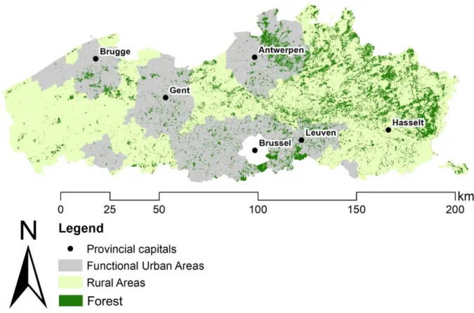
67
time (Cardinale et al., 2012).
68
Tree diversity has been studied at genus level before (Hoover et al., 2017; Hope et al., 2003)
69
and might become more popular with increasing availability of observations from citizen
70
science (Dobbs et al., 2018). Observations of trees through citizen science initiatives have been
71
found to be more accurate at genus level than at species level (Roman et al., 2017). Plant
genus-72
level diversity is strongly linked to plant species-level diversity (O’Brien et al., 1998).
73
Additionally, interactions with host plants often occur at genus level and therefore genus level
74
diversity is also relevant for insect diversity (Kemp and Ellis, 2017), or ectomycorrhizal fungal
75
diversity (Gao et al., 2013). Thomsen et al. (2016) emphasize that a healthy urban tree
76
population requires a high generic diversity. Modelling tree diversity at genus level is thus of
77
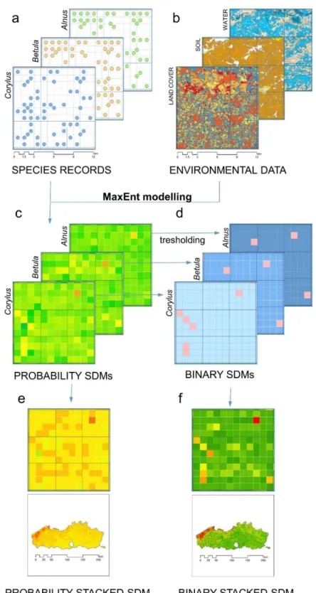
high value because it encompasses more reliable observation data and allows for diverse
78
applications.
79
Genus-level presence-only data can be used in species distribution models (SDMs). SDMs
80
correlate species observations and environmental covariates to predict habitat suitability (Elith
81
et al., 2006). Applications of SDMs are manifold: identifying species distributions, studying 82
impact of climate and land use change scenarios (Dyderski et al., 2018) and identifying areas
83
of interest for conservation (McCune, 2016). Applications of SDMs in urbanized areas are not
84
common (Della Rocca et al., 2017), yet they have been successfully applied in urban green
85
spaces (Milanovich et al., 2012) and human-dominated landscapes (McCune, 2016).
86
Species richness can be modelled by stacking individual SDMs on top of one another to yield
87
a total richness. Stacking of SDMs is most commonly done after thresholding the continuous
88
probability output of the individual SDMs, a method known as binary stacking (Calabrese et
89
al., 2014). Nevertheless, discretizing continuous probabilities using fixed thresholds (for 90
example considering all cases with a modelled probability of p > 0.55 as being present) is
91
generally discouraged (Merow et al., 2013). Instead, species-specific threshold rules can be
92
applied (Cao et al., 2013). Still, the literature suggests that binary stacking tends to
93
overestimate species richness because biotic limitations are not accounted for (Calabrese et al.,
94
2014; Gavish et al., 2017; Guisan and Rahbek, 2011). Nonetheless, combining binary SDMs
95
is the most straightforward method to create species richness maps (Trotta-Moreu & Lobo,
96
2010). Combining continuous probability data, which is called probability stacking, is an
97
alternative stacking approach (Calabrese et al., 2014), although interpretations are less
98
straightforward. Guisan & Rahbek (2011) have proposed a framework for spatially explicit
99
species assemblage modelling (SESAM). In the SESAM framework, a macro-ecological model
100
limits the number of species that can co-occur in one cell. One way of defining the
macro-101
ecological constraint is by stacking the probabilities of SDMs (probability stacking). D’Amen
102
et al. (2015) reduced overestimation by applying probability stacking successfully in the Alps 103
of western Switzerland at a fine spatial resolution.
104
In this study, we test a stratified approach, in which we run separate SDMs for rural and urban
105
areas in a mosaic landscape, to model tree diversity at genus level. We evaluate which
106
environmental covariates drive the urban and rural models. First, we hypothesize that different
environmental covariates drive the urban and rural models. We expect that soil nutrients and
108
soil moisture determine vegetation in rural areas, because this vegetation resembles the
109
potential natural vegetation more closely (Walthert and Meier, 2017). For urban areas we
110
expect an anthropogenic influence on the vegetation composition (Bourne and Conway, 2014).
111
Second, we hypothesize that the application of a macro-ecological constraint to take biotic
112
interactions into account would improve models for rural areas, but not for urban areas. We
113
expect that biotic interactions are more relevant in rural areas (D’Amen et al., 2015). Third, we
114
hypothesize that binary stacking performs sufficiently well in urban areas. We expect that
115
biotic interactions are less relevant in urban areas because of human intervention.
116 117
2. Materials and methods
118
2.1. Study area and stratification 119
Flanders is the northernmost of the three administrative regions of Belgium with an area of
120
13,522 km2 and a population density of 482 inhabitants per km2. The area has a north-south
121
soil gradient of decreasing fraction of sand and increasing fraction of silt. The climate
122
according to Köppen is a maritime temperate climate (Cfb) (Peel et al., 2007). The
123
Organization for Economic Co-operation and Development (OECD) considers Flanders
124
entirely as urbanized (Vervoort, 2016). Nevertheless, based on the Urban Audit of 2018
125
published by Eurostat, core cities and functional urban areas (FUAs) are delineated for
126
Flanders. The delineation is used to distinguish dominantly urban areas from more rural areas
127
in Flanders (Fig. 1). FUAs define a metropolitan area outside the geographical city boundaries,
128
taking into account demographic, economic and environmental factors (Khalili et al., 2018). In
129
Flanders, the FUAs are located around the capitals of each province, except for Hasselt (Fig.
130
1). Hasselt is a provincial capital located in the east of the region where forest cover is higher.
131
As only 10.6% of the study area consists of forest (De Keersmaeker et al., 2015), other (urban)
green spaces are of high importance for biodiversity (Aronson et al., 2017; Lepczyk et al.,
133
2017). Green space is most commonly defined as a vegetated area (Taylor and Hochuli, 2017).
134
We will focus on vegetated areas containing woody vegetation. The Belgian and Luxemburg
135
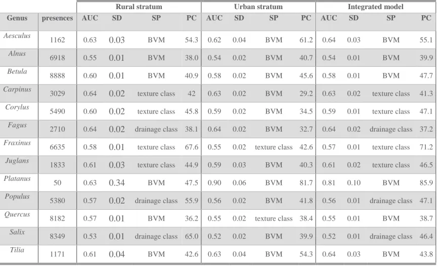
Institute for Floristics (IFBL) developed a regular grid of 4×4 km squares further divided into
136
1×1 km squares covering Belgium and Luxemburg. This grid is used as a reference for mapping
137
species distributions (Van Rompaey, 1943). In this study the 1×1 km IFBL grid is used to mask
138
observation data and environmental covariates.
139
140
Fig. 1: Stratification of the Region of Flanders into functional urban areas and rural areas 141
according to the Urban Audit of Eurostat (2018). The provincial capital cities are labeled and the 142
forest cover in the region is visualized. 143
2.2. Species distribution modelling 144
Species distribution models (SDMs) estimate the relationship between recorded occurrences at
145
sites (samples) and the environmental and/or spatial characteristics of those sites
146
(environmental covariates) (Elith et al., 2011). This relationship is then used to predict
147
occurrences elsewhere. In the stratified approach, separate SDMs are run for the urban and
148
rural strata. Subsequently, the urban and rural data are combined in an integrated approach to
form a model that covers the whole region of Flanders. The models are validated with
150
independent field data to evaluate their utility in the urban and rural strata. The workflow for
151
the integrated approach, which is parallel for the stratified approach, is visualized in Fig. 2 and
152
explained in the following sections.
153
2.2.1. Occurrence data
The occurrence data of thirteen tree genera were included in the study: Aesculus (horse
154
chestnut), Alnus (alder), Betula (birch), Carpinus (hornbeam), Corylus (hazel), Fagus (beech),
155
Fraxinus (ash), Juglans (walnut), Platanus (plane), Populus (poplar), Quercus (oak), Salix 156
(willow) and Tilia (linden). Presence-records of these genera were extracted from Florabank1
157
(Van Landuyt & Brosens, 2017) available on GBIF.org. The Florabank is an open-access
158
presence-only database of validated observations of vascular plants, from checklists, literature
159
and herbarium specimen information. The observations are georeferenced and attributed to the
160
centers of 14317 1km×1km IFBL grid cells (Van Landuyt et al., 2012).
161 162 163
Fig. 2: Mapping tree diversity at the genus level from presence-only and environmental data. Presence-only data from Florabank (a) and environmental data from various sources (b) are combined in a Species Distribution Model (SDM) using MaxEnt. The continuous output of MaxEnt, probability models (c), can be converted to presence-absence models (binary SDMs) by applying genus specific thresholds (d). Stacking the probability models and applying the probability ranking rule results in a probability stacked SDM (e). Aggregating the thresholded SDMs results in a binary stacked SDM (f).
2.2.2. Environmental covariates 164
Soil texture class, soil drainage class, mean lowest and highest groundwater table depth, land
165
cover type and habitat type were the environmental covariates used. In Belgium, natural plant
166
communities are primarily determined by variation in soil nutrient content and soil moisture
167
(Cornelis et al., 2009). Thus, soil texture and drainage class were extracted as categorical soil
168
variables from the Belgian soil map (Dondeyne et al., 2014). This vector geodataset was first
169
resampled to a raster, using the IFBL grid as the mask layer and the cell assignment type
170
‘maximum combined area’. The ‘maximum combined area’ rule selects the attribute value from
171
the polygon with the largest total area overlapping with the grid cell (ESRI, 2017). Mean
172
highest and lowest groundwater tables data were obtained from a soil hydrology raster
173
(ECOPLAN, 2014) and resampled to the IFBL grid.
174
Land cover data were obtained from one of the base layers in the ECOPLAN ecosystem
175
services information system (ECOPLAN, 2014). The geodataset contains a basic land cover
176
classification (the list of classes is available in Appendix 1). The grid with a spatial resolution
177
of 5m was resampled to the IFBL grid, retaining the land cover with the largest area in the grid
178
cell.
179
Habitat data were obtained from the Biological Valuation Map (BVM), a geodataset of habitat
180
types with attribute information on the ecological context and value of the delineated areas
181
(Vriens et al., 2011). The BVM contains information about heterogeneity of urban areas, such
182
as the density and context of built-up areas, industrial areas and recreational areas. The classes
183
of the BVM are listed in Appendix 1. The BVM is a vector geodataset and was resampled to
184
the IFBL grid using ‘maximum combined area’ as the cell assignment type. Resampling and
185
masking of the environmental geodatasets were performed in ArcGIS 10.5.1-software (ESRI,
186
Redlands, CA, 2017).
187
2.2.3. Probability models 188
Probability models of the spatial distribution of each of the 13 genera were developed using
189
MaxEnt version 3.3.3k. MaxEnt is a machine‐learning algorithm highly suitable to develop
190
models from presence-only data (Elith et al., 2006; Phillips et al., 2006). The algorithm is based
191
on the principles of maximum entropy and finds an optimal probability distribution using a
192
combination of occurrence data and environmental data (Elith et al., 2011). MaxEnt is known
193
to perform well even when environmental covariates are linearly correlated (De Marco and
194
Nóbrega, 2018). The logistic output of MaxEnt is an attempt at expressing the raw output as a
195
probability of presence (Elith et al., 2011). A 10-fold cross validation was applied. Model
196
performance was assessed with the area under the receiver operating characteristic curve
197
(AUC) statistic, ranging between 0 and 1. When AUC values are higher than 0.5, the model
198
performs better than a random distribution. For every genus, three models were developed: one
199
using the entire dataset (integrated approach), then one for the rural and one for the urban areas
200
(stratified approach). To evaluate the driving factors in these models, we determined the
201
environmental covariate with the highest percentage of contribution to the model.
202 203
2.2.4. Binary stacking 204
We applied the ‘10 percentile training presence’ rule on the MaxEnt-output (Ficetola et al.,
205
2009; Pearson et al., 2006; Skowronek et al., 2017), for every genus and model approach
206
separately, resulting in a threshold value above which 90% of the training samples are correctly
207
classified. Thus, a unique threshold value is used for every genus to create a binary output (0
208
= absence, 1 = presence). Binary stacking is the process of adding up the individual binary
209
models, resulting in a generic tree diversity varying from 0 to 13 genera.
210 211
2.2.5. Probability stacking 212
As a cell-specific macro-ecological constraint we summed the MaxEnt-probabilities per grid
213
cell (D’Amen et al., 2015), resulting in a possible generic tree diversity range between 1.96
214
and 8.76. To determine which genera occur in the constrained cells we used the ‘probability
215
ranking’ rule. The genera are assigned to the cell according to decreasing order of probability
216
of presence determined from the SDMs (2.2.3), until the cell-specific macro-ecological
217
constraint is reached. Probability ranking as described in the SESAM framework is
218
incorporated in the package ‘ecospat’ available for R (Di Cola et al., 2017) and was executed
219
with R software 3.4.3 (R Core Team, 2017).
220 221
2.3. Validation 222
The probability models (2.2.3) were cross-validated before they were stacked. In addition, the
223
stacked models were validated with independent field data. The independent field data
224
consisted of recordings of the genus’s occurrence around 208 randomly selected point
225
locations, with a search effort per point of ten minutes with two observers. The sampling
226
protocol is derived from the timed-meander sampling protocol (Goff et al., 1982), which is
227
applied in various fields of ecology (Threlfall et al., 2017) and is favored because of its
cost-228
effectiveness (Hamm, 2013). The 208 point locations are distributed over 130 IFBL cells.
229
There are 87 rural cells and 43 urban cells. A genus is present in a cell if it is observed in at
230
least one of the random point locations within the cell. The field data are assumed to provide
231
the true condition that is compared to the predicted condition provided by the SDMs at genus
232
level. True condition data and predicted condition data were compared in a confusion matrix,
233
describing true positive (TP), true negative (TN), false positive (FP) and false negative (FN)
234
outcomes. Based on the values in the confusion matrix, we evaluated the model performance
235
by calculating the true positive rate (TPR). TPR is the number of true positives divided by the
236
total of positive cases, the sum of true and false positives. The TPR informs simultaneously
about the presences that are correctly predicted and about those that were incorrectly identified
238
as positives. A TPR of 80% would indicate that 80% of the presences are true positives while
239
20% are false positives. However, in the present study, the false positives are not necessarily
240
false as the species could have been missed during the validation field work. Therefore we
241
focus on the true positives when interpreting the TPR. Additionally, the percentage of false
242
negatives is included in the evaluation, because this percentage provides information on the
243
underestimation of the stacking method. The higher the percentage of false negatives, the more
244
the tree diversity at genus level is underestimated.
245 246
2.4 Compare model outcomes 247
To compare model outcomes we calculated average modelled tree diversity at genus level and
248
95% confidence intervals for binary stacked vs. probability stacked models and for integrated
249
vs. stratified approaches and for urban vs. rural areas. We used the paired sample t-test (with a
250
statistical cutoff value of 0.05) to test whether overall average modelled tree diversity at genus
251
level differed between binary stacked and probability stacked models. We then used the paired
252
sample t-test to test whether modelled generic tree diversity differed between integrated and
253
stratified approaches within the binary stacked models, both for the entire dataset and for a
254
dataset stratified in urban vs. rural areas.
255 256
3. Results
257
3.1 Probability models 258
The species distribution models outperformed the random spatial distribution (all AUC > 0.5;
259
Table 1), for the stratified approach as well as the integrated approach. On average the AUC is
260
0.60 with a standard deviation of 0.007. The strength of the strongest predictor ranges from
261
32.7-85.7 percent of contribution (Table 1). For 11 out of 13 urban models, the strongest
262
predictor is the Biological Valuation Map (BVM), containing information on urban
263
heterogeneity. For the rural model as well as the integrated model, we found that for some
264
genera the strongest predictors were the soil variables texture class and drainage class.
Table 1: Summary of the species distribution models for each genus. Reporting the number of grid cells occupied by an observation (presences), the average area under the curve (AUC) as a measure to evaluate the models, the standard deviation of the AUC (SD), the strongest predictor (SP) and the percent of contribution (PC) of this strongest predictor to the MaxEnt model. (BVM = Biological Valuation Map)
Rural stratum Urban stratum Integrated model
Genus presences AUC SD SP PC AUC SD SP PC AUC SD SP PC
Aesculus 1162 0.63 0.03 BVM 54.3 0.62 0.04 BVM 61.2 0.64 0.03 BVM 55.1 Alnus 6918 0.55 0.01 BVM 38.0 0.54 0.02 BVM 40.7 0.54 0.01 BVM 39.9 Betula 8888 0.60 0.01 BVM 40.9 0.58 0.02 BVM 45.6 0.58 0.01 BVM 47.7 Carpinus
3029 0.64 0.02 texture class 42 0.63 0.02 BVM 29.2 0.63 0.02 texture class 41.3
Corylus
5490 0.60 0.02 texture class 45.8 0.59 0.02 BVM 34.5 0.59 0.01 texture class 47.1
Fagus
2710 0.64 0.02 drainage class 38.1 0.64 0.02 BVM 32.7 0.64 0.02 drainage class 37.2
Fraxinus
6635 0.58 0.01 texture class 67.6 0.55 0.02 texture class 42.6 0.57 0.01 texture class 71.2
Juglans
1833 0.61 0.03 texture class 44.9 0.59 0.03 BVM 40.3 0.61 0.02 texture class 46.5
Platanus
50 0.63 0.34 BVM 47.5 0.90 0.06 BVM 81.7 0.81 0.10 BVM 85.9
Populus
5380 0.57 0.02 drainage class 55.9 0.56 0.02 BVM 41.8 0.56 0.01 drainage class 47.1
Quercus
8182 0.57 0.01 BVM 36.2 0.55 0.02 texture class 38.4 0.55 0.01 BVM 38.7
Salix
8349 0.53 0.01 drainage class 65.0 0.52 0.02 BVM 39.9 0.52 0.01 drainage class 46.4
Tilia
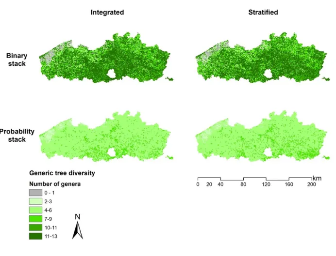
3.2 Stacked species distribution models
For the integrated as well as the stratified approach binary stacking resulted in a generic tree diversity varying between 0 and 13. Probability stacking resulted in a lower generic tree diversity between 2 and 9 (Fig. 3). Spatial differences in generic tree diversity between the integrated and the stratified approach are not strongly pronounced.
Fig. 3: Tree diversity at genus level determined by binary (upper) and probability (lower) stacking of the MaxEnt models developed in an integrated (left) and stratified (right) modelling approach. The cell size is 1km×1km.
3.3 Validation
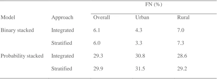
The binary stacking method, with an overall TPR of 0.90, performed better than the probability stacking method, with a considerably lower overall TPR of 0.52-0.53 (Table 2). Overall, the integrated and the stratified approach performed equally well. The binary stacking method had a lower percentage of false negatives (6.0 - 6.1 %) than the probability stacking method (29.3 – 29.9 %) (Table 3).
Table 2: Validation results: true positive rate (TPR) derived from the confusion matrix.
TPR
Model Approach Overall Urban Rural Binary stacked Integrated 0.90 0.94 0.89
Stratified 0.90 0.95 0.88 Probability stacked Integrated 0.53 0.54 0.53 Stratified 0.52 0.53 0.53
Table 3: Validation results: percentage of false negatives (%) derived from the confusion matrix.
FN (%)
Model Approach Overall Urban Rural
Binary stacked Integrated 6.1 4.3 7.0
Stratified 6.0 3.3 7.3
Probability stacked Integrated 29.3 30.8 28.6
3.4 Comparison of model outcomes
3.4.1 Binary stacking vs. probability stacking
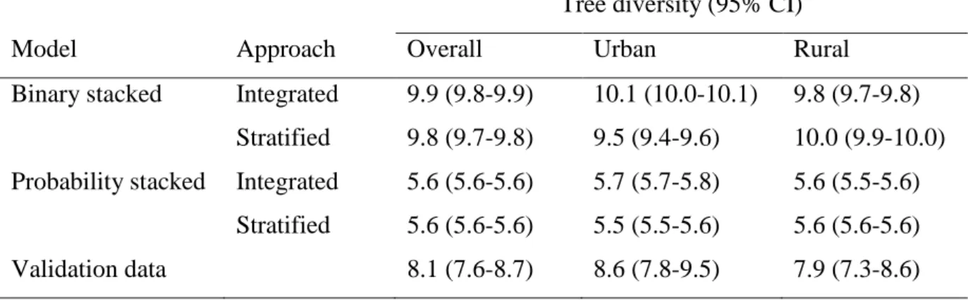
The overall average tree diversity at genus level was higher for binary stacked models (9.8-9.9) than for probability stacked models (5.6) (Table 4). The diversity based on the validation data was 8.1, in line with results from the binary stacking approach. There was a significant mean difference of 4.3 (95% CI 4.2-4.3) between binary stacked and probability stacked models for the integrated approach (paired t-test t = 200.1, df = 13458, p < 0.001). There was a significant mean difference of 4.2 (95% CI 4.1-4.3) between binary and probability stacked models for the stratified approach (paired t-test t = 153.7, df = 13458, p < 0.001).
Table 4: Average modelled tree diversity at genus level based on binary and probability stacked models, for integrated and stratified approaches and for urban and rural areas.
Tree diversity (95% CI) Model Approach Overall Urban Rural
Binary stacked Integrated 9.9 (9.8-9.9) 10.1 (10.0-10.1) 9.8 (9.7-9.8) Stratified 9.8 (9.7-9.8) 9.5 (9.4-9.6) 10.0 (9.9-10.0) Probability stacked Integrated 5.6 (5.6-5.6) 5.7 (5.7-5.8) 5.6 (5.5-5.6)
Stratified 5.6 (5.6-5.6) 5.5 (5.5-5.6) 5.6 (5.6-5.6) Validation data 8.1 (7.6-8.7) 8.6 (7.8-9.5) 7.9 (7.3-8.6)
3.4.2 Binary stacking: rural vs. urban areas
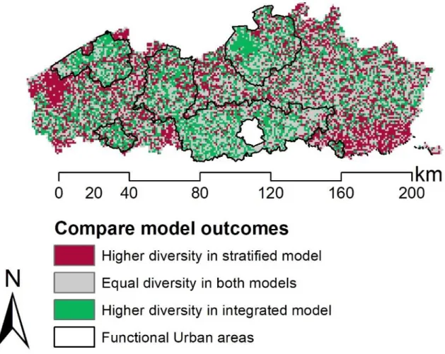
For binary stacked models, the integrated approach yielded a statistically significant higher overall estimated tree diversity at genus level [mean difference integrated vs. stratified 0.09 (95% CI 0.06-0.11), t = 6.72, df = 13458, p<0.001]. However, subtracting the stratified result from the integrated result revealed a spatial differentiation (Fig. 4). The stratified approach resulted in a significantly higher diversity in the rural areas, thus a negative mean difference of –0.18 (95% CI -0.21 – -0.15) (t = -12.5, df = 8359, p<0.001). The integrated approach, however, resulted in a significantly higher diversity in the urban areas, thus a positive mean difference of 0.52 (95% CI 0.48-0.57) (t = 22.3, df = 5098, p<0.001).
Green pixels (Fig. 4) represent a higher diversity obtained with the integrated approach. These green pixels are often clustered within the FUAs (black outline, Fig. 4). Conversely, red pixels represent a higher diversity obtained with the stratified approach. These red pixels are observed in clusters outside the FUAs, especially in extremely rural areas such as: ‘De Westhoek’ in the west and ‘Haspengouw’ in the south-east of Flanders (Fig. 4).
Fig. 4: The difference in the binary stacking results from the integrated and stratified approach. Cell size is 1km×1km.
4. Discussion and conclusions 4.1 Environmental covariates
Rural and urban models were driven by different environmental covariates, which confirms the first hypothesis. As expected, soil variables, such as texture class and drainage class, were of high importance to explain the distribution of native trees in rural areas. Texture class was an important covariate for Corylus, for example, because this genus requires richer loamy soils (Özenç, 2001). Salix and Populus can tolerate wet soils (Zalesny and Bauer, 2007) and as a result drainage class was an important environmental covariate in their SDMs. Earlier studies demonstrated that including soil factors in plant SDMs results in improved predictions (Buri et al., 2017). For urban areas we expected that the vegetation would be determined by anthropogenic influences. The urban heterogeneity, which is better described in the Biological Valuation Map (BVM), was the most important covariate in the urban SDMs (Table 1). In the BVM seven urban/built up types are included (ua, ud, un, ur, uv, uc and ui), while the the other land cover map (ECOPLAN) contains only three urban land cover types (9101, 9201, 9202) (see Appendix 1). It has been emphasized in the past that including environmental covariates that account for the diverse functions of urban areas is important to understand urban plant species patterns (Godefroid and Koedam, 2007). Future developments of species distribution models in urban areas need to include covariates that address the variety of anthropogenic influence.
4.2 Stacking methods
At a fine spatial resolution, as in the work of D’Amen et al. (2015), binary stacking overestimates species diversity in a natural environment, because dispersal limitations and biotic interactions are not taken into account. In this study, however, we worked at a spatial resolution of 1km×1km and biotic interactions are less important at this relatively coarse resolution (Thuiller et al., 2015). The probability stacking method should prevent from overestimating tree diversity at genus level. Nevertheless, the low true positive rate (Table 2)
and the high percentage of false negatives (Table 3) showed that the probability stacking method underestimated tree diversity in Flanders. Additionally, in urbanized areas, human decision-making and management most likely override natural species selection and biotic interactions are therefore less likely to drive species composition. Therefore, binary stacking is the preferred method for biodiversity modelling at 1km×1km resolution in both urban areas and rural areas. Nevertheless, the scale-dependent applicability of a macro-ecological constraint needs further research as there is, to our knowledge, no literature on this topic.
4.3 Comparison of model outcomes
Binary stacking resulted in a significantly higher diversity at genus level compared to probability stacking (Table 4). This difference is not an overestimation of binary stacking, but due to an underestimation of probability stacking. Using the binary stacking method and the stratified approach, higher diversity was clustered in the rural areas (Table 4 and Fig. 4). Rural areas are thus more prone to overestimation and would probably benefit more from applying ecological constraints, compared to urban areas. Nevertheless, applications of macro-ecological constraints seem to be of higher relevance in more natural areas (D’Amen et al., 2015), far less urbanized than the rural areas in Flanders.
To conclude, we find that binary stacking is most suitable for both urban and rural areas in Flanders. Stratification of the study area did not improve model quality considerably, but confirmed that different environmental covariates contributed to the models of urban and rural areas. Probability stacking is to be considered in natural areas, but does not perform well in urbanized areas, especially at the moderate spatial resolution of 1km×1km.
4.4 Limitations
All Species Distribution Models (SDMs) had relatively low Area Under the Curve values (average AUC: 0.60± 0.01), but all performed better than random distributions (Table 1). By
stacking SDMs, errors in individual species models accumulate and degrade predictions of species diversity (D’Amen et al., 2015; Pottier et al., 2013). The importance of the BVM as an environmental covariate emphasizes the relevance of including urban heterogeneity in SDMs. Unfortunately, at a moderate resolution of 1×1km relevant intra-urban variation of the tree canopy (Weinberger et al., 2016) cannot be observed.
4.5 Applications
The model resulting from this study can be expanded by stacking more binary SDMs, by producing species-level models or by producing models of other plant groups. Spatially-explicit biodiversity data are vital for emerging environmental health studies (McInnes et al., 2017), for example to study relationships between residential and dynamic exposure and human health outcomes (Cox et al., 2017; Shanahan et al., 2016). Hjort et al. (2016) present a concept to calculate individual long-term or life time exposure to pollen with geographic information systems. Landscape and urban planners could also use tree diversity maps to identify areas with low diversity and optimize the delivery of ecosystem services or decrease potential social inequalities in access to biodiverse green space by increasing biodiversity in focus areas (Wolch et al., 2014). Finally, when subsets of models for allergenic species are used, diversity maps could be interpreted as allergy risk maps and inform pollen allergy patients about pollen allergy risks (McInnes et al., 2017).
References
Alvey, A.A., 2006. Promoting and preserving biodiversity in the urban forest. Urban For. Urban Green. 5, 195–201. https://doi.org/10.1016/J.UFUG.2006.09.003
Aronson, M.F., Lepczyk, C.A., Evans, K.L., Goddard, M.A., Lerman, S.B., MacIvor, J.S., Nilon, C.H., Vargo, T., 2017. Biodiversity in the city: key challenges for urban green space management. Front. Ecol. Environ. 15, 189–196. https://doi.org/10.1002/fee.1480
Buri, A., Cianfrani, C., Pinto-Figueroa, E., Yashiro, E., Spangenberg, J.E., Adatte, T., Verrecchia, E., Guisan, A., Pradervand, J.-N., 2017. Soil factors improve predictions of plant species distribution in a mountain environment. Prog. Phys. Geogr. 41, 703–722. https://doi.org/10.1177/0309133317738162
Calabrese, J.M., Certain, G., Kraan, C., Dormann, C.F., 2014. Stacking species distribution models and adjusting bias by linking them to macroecological models. Glob. Ecol. Biogeogr. 23, 99–112. https://doi.org/10.1111/geb.12102
Cao, Y., DeWalt, R.E., Robinson, J.L., Tweddale, T., Hinz, L., Pessino, M., 2013. Using Maxent to model the historic distributions of stonefly species in Illinois streams: The effects of regularization and threshold selections. Ecol. Modell. 259, 30–39. https://doi.org/10.1016/J.ECOLMODEL.2013.03.012
Cardinale, B.J., Duffy, J.E., Gonzalez, A., Hooper, D.U., Perrings, C., Venail, P., Narwani, A., Mace, G.M., Tilman, D., Wardle, D.A., Kinzig, A.P., Daily, G.C., Loreau, M., Grace, J.B., Larigauderie, A., Srivastava, D.S., Naeem, S., 2012. Biodiversity loss and its impact on humanity. https://doi.org/10.1038/nature11148
Cornelis, J., Hermy, M., Roelandt, B., De Keersmaeker, L., Vandekerkhove Kris, 2009. Bosplantengemeenschappen in Vlaanderen, eEen typologie van bossen gebasseerd op de kruidlaag. INBO.M.2009.5. Agentschap voor Natuur en Bos en Intituut voor Natuur- en Bosonderzoek, Brussel.
Cox, D.T.C., Bennie, J., Casalegno, S., Hudson, H.L., Anderson, K., Gaston, K.J., 2019. Skewed contributions of individual trees to indirect nature experiences. Landsc. Urban
Plan. 185, 28–34. https://doi.org/10.1016/J.LANDURBPLAN.2019.01.008
D’Amen, M., Dubuis, A., Fernandes, R.F., Pottier, J., Pellissier, L., Guisan, A., 2015. Using species richness and functional traits predictions to constrain assemblage predictions from stacked species distribution models. J. Biogeogr. 42, 1255–1266. https://doi.org/10.1111/jbi.12485
De Keersmaeker, L., Onkelinx, T., De Vos, B., Rogiers, N., Vandekerkhove, K., Thomaes, A., De Schrijver, A., Hermy, M., Verheyen, K., 2015. The analysis of spatio-temporal forest changes (1775–2000) in Flanders (northern Belgium) indicates habitat-specific levels of fragmentation and area loss. Landsc. Ecol. 30, 247–259. https://doi.org/10.1007/s10980-014-0119-7
De Marco, P., Nóbrega, C.C., 2018. Evaluating collinearity effects on species distribution models: An approach based on virtual species simulation. PLoS One 13, e0202403. https://doi.org/10.1371/journal.pone.0202403
Della Rocca, F., Bogliani, G., Milanesi, P., 2017. Patterns of distribution and landscape connectivity of the stag beetle in a human-dominated landscape. Nat. Conserv. 19, 19–37. https://doi.org/10.3897/natureconservation.19.12457
Di Cola, V., Broennimann, O., Petitpierre, B., Breiner, F.T., D’Amen, M., Randin, C., Engler, R., Pottier, J., Pio, D., Dubuis, A., Pellissier, L., Mateo, R.G., Hordijk, W., Salamin, N., Guisan, A., 2017. ecospat: an R package to support spatial analyses and modeling of species niches and distributions. Ecography (Cop.). 40, 774–787. https://doi.org/10.1111/ecog.02671
Dobbs, C., Hernández, A., de la Barrera, F., Miranda, M.D., Paecke, S.R., 2018. Integrating Urban Biodiversity Mapping, Citizen Science and Technology, in: Urban Biodiversity. Routledge, pp. 236–247. https://doi.org/10.9774/GLEAF.9781315402581_16
Dondeyne, S., Vanierschot, L., Langohr, R., Ranst, E. Van, Deckers, J., 2014. The soil map of the Flemish region converted to the 3rd edition of the World Reference Base for soil resources 139.
Donovan, R.G., Stewart, H.E., Owen, S.M., MacKenzie, A.R., Hewitt, C.N., 2005. Development and Application of an Urban Tree Air Quality Score for Photochemical Pollution Episodes Using the Birmingham, United Kingdom, Area as a Case Study. Environ. Sci. Technol. 39, 6730–6738. https://doi.org/10.1021/ES050581Y
Dyderski, M.K., Paź, S., Frelich, L.E., Jagodziński, A.M., 2018. How much does climate change threaten European forest tree species distributions? Glob. Chang. Biol. 24, 1150– 1163. https://doi.org/10.1111/gcb.13925
ECOPLAN, 2014. ECOPLAN Monitor [WWW Document]. URL
http://www.ecosysteemdiensten.be/cms/
Elith, J., H. Graham, C., P. Anderson, R., Dudík, M., Ferrier, S., Guisan, A., J. Hijmans, R., Huettmann, F., R. Leathwick, J., Lehmann, A., Li, J., G. Lohmann, L., A. Loiselle, B., Manion, G., Moritz, C., Nakamura, M., Nakazawa, Y., McC. M. Overton, J., Townsend Peterson, A., J. Phillips, S., Richardson, K., Scachetti-Pereira, R., E. Schapire, R., Soberón, J., Williams, S., S. Wisz, M., E. Zimmermann, N., 2006. Novel methods improve prediction of species’ distributions from occurrence data. Ecography (Cop.). 29, 129–151. https://doi.org/10.1111/j.2006.0906-7590.04596.x
Elith, J., Phillips, S.J., Hastie, T., Dudík, M., Chee, Y.E., Yates, C.J., 2011. A statistical explanation of MaxEnt for ecologists. Divers. Distrib. 17, 43–57. https://doi.org/10.1111/j.1472-4642.2010.00725.x
ESRI, 2017. ESRI, Redlands, US. http://www.esri.com/software/arcgis. last accessed 23/09/2017.
Ficetola, G.F., Thuiller, W., Padoa-Schioppa, E., 2009. From introduction to the establishment of alien species: bioclimatic differences between presence and reproduction localities in the slider turtle. Divers. Distrib. 15, 108–116. https://doi.org/10.1111/j.1472-4642.2008.00516.x
Gao, C., Shi, N.-N., Liu, Y.-X., Peay, K.G., Zheng, Y., Ding, Q., Mi, X.-C., Ma, K.-P., Wubet, T., Buscot, F., Guo, L.-D., 2013. Host plant genus-level diversity is the best predictor of
ectomycorrhizal fungal diversity in a Chinese subtropical forest. Mol. Ecol. 22, 3403– 3414. https://doi.org/10.1111/mec.12297
Gavish, Y., Marsh, C.J., Kuemmerlen, M., Stoll, S., Haase, P., Kunin, W.E., 2017. Accounting for biotic interactions through alpha-diversity constraints in stacked species distribution models. Methods Ecol. Evol. 8, 1092–1102. https://doi.org/10.1111/2041-210X.12731 Godefroid, S., Koedam, N., 2007. Urban plant species patterns are highly driven by density and
function of built-up areas. Landsc. Ecol. 22, 1227–1239. https://doi.org/10.1007/s10980-007-9102-x
Goff, F.G., Dawson, G.A., Rochow, J.J., 1982. Site examination for threatened and endangered plant species. Environ. Manage. 6, 307–316. https://doi.org/10.1007/BF01875062
Guisan, A., Rahbek, C., 2011. SESAM - a new framework integrating macroecological and species distribution models for predicting spatio-temporal patterns of species assemblages. J. Biogeogr. 38, 1433–1444. https://doi.org/10.1111/j.1365-2699.2011.02550.x
Hamm, C.A., 2013. Estimating abundance of the federally endangered Mitchell’s satyr butterfly using hierarchical distance sampling. Insect Conserv. Divers. 6, 619–626. https://doi.org/10.1111/icad.12017
Hjort, J., Hugg, T.T., Antikainen, H., Rusanen, J., Sofiev, M., Kukkonen, J., Jaakkola, M.S., Jaakkola, J.J.K., 2016. Fine-Scale Exposure to Allergenic Pollen in the Urban Environment: Evaluation of Land Use Regression Approach. Environ. Health Perspect. 124, 619–26. https://doi.org/10.1289/ehp.1509761
Hoover, J.D., Kumar, S., James, S.A., Liesz, S.J., Laituri, M., 2017. Modeling hotspots of plant diversity in New Guinea. Trop. Ecol. 58, 623–640.
Hope, D., Gries, C., Zhu, W., Fagan, W.F., Redman, C.L., Grimm, N.B., Nelson, A.L., Martin, C., Kinzig, A., 2003. Socioeconomics drive urban plant diversity, PNAS.
Hüse, B., Szabó, S., Deák, B., Tóthmérész, B., 2016. Mapping an ecological network of green habitat patches and their role in maintaining urban biodiversity in and around Debrecen city (Eastern Hungary). Land use policy 57, 574–581.
https://doi.org/10.1016/J.LANDUSEPOL.2016.06.026
Kemp, J.E., Ellis, A.G., 2017. Significant local-scale plant-insect species richness relationship independent of abiotic effects in the temperate cape floristic region biodiversity hotspot. PLoS One 12. https://doi.org/10.1371/journal.pone.0168033
Khalili, A., van den Besselaar, P., de Graaf, K.A., 2018. Using Linked Open Geo Boundaries for Adaptive Delineation of Functional Urban Areas. Springer, Cham, pp. 327–341. https://doi.org/10.1007/978-3-319-98192-5_51
Konarska, J., Uddling, J., Holmer, B., Lutz, M., Lindberg, F., Pleijel, H., Thorsson, S., 2016. Transpiration of urban trees and its cooling effect in a high latitude city. Int. J. Biometeorol. 60, 159–172. https://doi.org/10.1007/s00484-015-1014-x
Lee, H., Mayer, H., Chen, L., 2016. Contribution of trees and grasslands to the mitigation of human heat stress in a residential district of Freiburg, Southwest Germany. Landsc. Urban Plan. 148, 37–50. https://doi.org/10.1016/j.landurbplan.2015.12.004
Lepczyk, C.A., Aronson, M.F.J., Evans, K.L., Goddard, M.A., Lerman, S.B., MacIvor, J.S., 2017. Biodiversity in the City: Fundamental Questions for Understanding the Ecology of Urban Green Spaces for Biodiversity Conservation. Bioscience 67, 799–807. https://doi.org/10.1093/biosci/bix079
McCune, J.L., 2016. Species distribution models predict rare species occurrences despite significant effects of landscape context. J. Appl. Ecol. 53, 1871–1879. https://doi.org/10.1111/1365-2664.12702
McInnes, R.N., Hemming, D., Burgess, P., Lyndsay, D., Osborne, N.J., Skjøth, C.A., Thomas, S., Vardoulakis, S., 2017. Mapping allergenic pollen vegetation in UK to study environmental exposure and human health. Sci. Total Environ. 599–600, 483–499. https://doi.org/10.1016/J.SCITOTENV.2017.04.136
Merow, C., Smith, M.J., Silander, J.A., 2013. A practical guide to MaxEnt for modeling species’ distributions: what it does, and why inputs and settings matter. Ecography (Cop.). 36, 1058–1069. https://doi.org/10.1111/j.1600-0587.2013.07872.x
Milanovich, J.R., Peterman, W.E., Barrett, K., Hopton, M.E., 2012. Do species distribution models predict species richness in urban and natural green spaces? A case study using
amphibians. Landsc. Urban Plan. 107, 409–418.
https://doi.org/10.1016/J.LANDURBPLAN.2012.07.010
O’Brien, E.M., Whittaker, R.J., Field, R., 1998. Climate and woody plant diversity in southern Africa: relationships at species, genus and family levels. Ecography (Cop.). 21, 495–509. https://doi.org/10.1111/j.1600-0587.1998.tb00441.x
Özenç, D.B., 2001. Methods of determining lime requirements of soils in the eastern black sea
hazelnut growing region. Acta Hortic. 335–342.
https://doi.org/10.17660/ActaHortic.2001.556.50
Pearson, R.G., Raxworthy, C.J., Nakamura, M., Townsend Peterson, A., 2006. Predicting species distributions from small numbers of occurrence records: a test case using cryptic geckos in Madagascar. J. Biogeogr. 34, 102–117. https://doi.org/10.1111/j.1365-2699.2006.01594.x
Peel, M.C., Finlayson, B.L., Mcmahon, T.A., 2007. Updated world map of the Köppen-Geiger climate classification, Hydrology and Earth System Sciences Discussions, European Geosciences Union. https://doi.org/<hal-00305098>
Phillips, S.J., Anderson, R.P., Schapire, R.E., 2006. Maximum entropy modeling of species geographic distributions. Ecol. Modell. 190, 231–259. https://doi.org/10.1016/j.ecolmodel.2005.03.026
Pottier, J., Dubuis, A., Pellissier, L., Maiorano, L., Rossier, L., Randin, C.F., Vittoz, P., Guisan, A., 2013. The accuracy of plant assemblage prediction from species distribution models varies along environmental gradients. Glob. Ecol. Biogeogr. 22, 52–63. https://doi.org/10.1111/j.1466-8238.2012.00790.x
R Core Team (2017). R: A language and environment for statistical computing. R Foundation for Statistical Computing, Vienna, Austria. URL https://www.R-project.org/.
Sanders, J.R., Betz, D.R., Jordan, R.C., 2017. Data quality in citizen science urban tree inventories. Urban For. Urban Green. 22, 124–135. https://doi.org/10.1016/J.UFUG.2017.02.001
Salmond, J.A., Tadaki, M., Vardoulakis, S., Arbuthnott, K., Coutts, A., Demuzere, M., Dirks, K.N., Heaviside, C., Lim, S., Macintyre, H., McInnes, R.N., Wheeler, B.W., 2016. Health and climate related ecosystem services provided by street trees in the urban environment. Environ. Heal. 15, S36. https://doi.org/10.1186/s12940-016-0103-6
Scholz, T., Hof, A., Schmitt, T., 2018. Cooling Effects and Regulating Ecosystem Services Provided by Urban Trees—Novel Analysis Approaches Using Urban Tree Cadastre Data. Sustainability 10, 712. https://doi.org/10.3390/su10030712
Selmi, W., Weber, C., Rivière, E., Blond, N., Mehdi, L., Nowak, D., 2016. Air pollution removal by trees in public green spaces in Strasbourg city, France. Urban For. Urban Green. 17, 192–201. https://doi.org/10.1016/J.UFUG.2016.04.010
Skowronek, S., Ewald, M., Isermann, M., Van De Kerchove, R., Lenoir, J., Aerts, R., Warrie, J., Hattab, T., Honnay, O., Schmidtlein, S., Rocchini, D., Somers, B., Feilhauer, H., 2017. Mapping an invasive bryophyte species using hyperspectral remote sensing data. Biol. Invasions 19, 239–254. https://doi.org/10.1007/s10530-016-1276-1
Taylor, L., Hochuli, D.F., 2017. Defining greenspace: Multiple uses across multiple disciplines.
Landsc. Urban Plan. 158, 25–38.
https://doi.org/10.1016/J.LANDURBPLAN.2016.09.024
Thomsen, P., Bühler, O., Kristoffersen, P., 2016. Diversity of street tree populations in larger Danish municipalities. Urban For. Urban Green. 15, 200–210. https://doi.org/10.1016/J.UFUG.2015.12.006
Threlfall, C.G., Mata, L., Mackie, J.A., Hahs, A.K., Stork, N.E., Williams, N.S.G., Livesley, S.J., 2017. Increasing biodiversity in urban green spaces through simple vegetation interventions. J. Appl. Ecol. 54, 1874–1883. https://doi.org/10.1111/1365-2664.12876 Thuiller, W., Pollock, L.J., Gueguen, M., Münkemüller, T., 2015. From species distributions to
meta-communities. Ecol. Lett. 18, 1321–1328. https://doi.org/10.1111/ele.12526
Trotta-Moreu, N., Lobo, J.M., 2010. Deriving the Species Richness Distribution of Geotrupinae (Coleoptera: Scarabaeoidea) in Mexico From the Overlap of Individual Model Predictions. Environ. Entomol. 39, 42–49. https://doi.org/10.1603/EN08179
Van Landuyt, W., Vanhecke, L., Brosens, D., 2012. Florabank1: a grid-based database on vascular plant distribution in the northern part of Belgium (Flanders and the Brussels Capital region). PhytoKeys 12, 59–67. https://doi.org/10.3897/phytokeys.12.2849
Van Rompaey, E., 1943. Cartes Floristiques. Bull. la Société R. Bot. Belgique / Bull. van K. Belgische Bot. Ver. 75, 48–56. https://doi.org/10.2307/20791920
Vervoort, P., 2016. A healthy urban future for Flanders? Reducing the gap in knowledge for spatial policy and outlining consequences for governance, in: 10th AESOP YA Conference. AESOP, Ghent.
Vriens, L., De Knijf, G., De Saeger, S., Guelinckx, R., Oosterlynck, P., Van Hove, M., Paelinckx, D., 2011. De Biologische Waarderingskaart. Biotopen en hun verspreiding in Vlaanderen en het Brussels Hoofdstedelijk Gewest., in: Mededelingen van Het Instituut Voor Natuur- En Bosonderzoek. INBO.M.2011.1, Brussels, p. 416.
Weinberger, K.R., Kinney, P.L., Robinson, G.S., Sheehan, D., Kheirbek, I., Matte, T.D., Lovasi, G.S., 2016. Levels and determinants of tree pollen in New York City. J. Expo. Sci. Environ. Epidemiol. 28, 119. https://doi.org/10.1038/jes.2016.72
Wolch, J.R., Byrne, J., Newell, J.P., 2014. Urban green space, public health, and environmental justice: The challenge of making cities ‘just green enough.’ Landsc. Urban Plan. 125, 234– 244. https://doi.org/10.1016/J.LANDURBPLAN.2014.01.017
Zalesny, R.S., Bauer, E.O., 2007. Selecting and utilizing Populus and Salix for landfill covers: Implications for leachate irrigation. Int. J. Phytoremediation 9, 497–511. https://doi.org/10.1080/15226510701709689
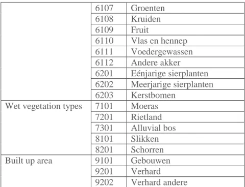
Appendix 1:
Table 1: Ecoplan land cover classification (in Dutch). Retrieved from:
https://www.uantwerpen.be/nl/onderzoeksgroep/ecoplan/ecoplan-tools/ecoplan-geoloket/
Complex Code Dutch name
water 10101 Stilstaand water
10201 Getijde mesohaline 10202 Getijde Oligohalien 10203 Getijde zoet
10204 Zoet 10301 Zee
Bush land 1101 Ruigten en pioniersvegetatie 1201 Struweel 1301 Struiken boomgaard 1302 Laagstam 1303 Hoogstam 1401 Ander hooggroen 1402 Ander laaggroen Forest complexes 2101 Berk
2102 Beuk 2103 Beuk – naaldhout 2104 Eik 2105 Eik – naaldhout 2106 Populier 2107 Populier – naaldhout 2108 Ander loofhout
2109 Ander loofhout – naaldhout 2201 lork
2202 Lork – loofhout 2203 Fijnspar
2204 Fijnspar – loofhout 2205 Zwarte den
2206 Zwarte den – loofhout 2207 Grove den
2208 Grove den – loofhout 2209 Ander naaldhout
2210 Ander naaldhout – loofhout Grasslands 3101 Voedselarm grassland
3102 Voedselrijk grassland 3201 Voedselrijk grasland Heath lands 4101 Droge heide
4201 Vochtige heide Bare soils 5101 Kale bodem
5201 Duinen 5301 Strand
5401 Niet verharde wegen Agricultural land 6101 Aardappel
6102 Mais 6103 Graan 6104 Zaden 6105 Peulvruchten 6106 Suikerbiet
6107 Groenten 6108 Kruiden 6109 Fruit 6110 Vlas en hennep 6111 Voedergewassen 6112 Andere akker 6201 Eénjarige sierplanten 6202 Meerjarige sierplanten 6203 Kerstbomen
Wet vegetation types 7101 Moeras 7201 Rietland 7301 Alluvial bos 8101 Slikken 8201 Schorren Built up area 9101 Gebouwen
9201 Verhard
9202 Verhard andere
Table 2: Biological valuation map classification of habitat types (in Dutch). Retreived from: https://www.geopunt.be/catalogus/datasetfolder/bf31d5c7-e97d-4f71-a453-5584371e7559
Complex Code(s) Dutch name
Stagnant water ad Bezinkingsbekken ae, aer, aev Eutroof
ap, apo, app Diep of zeer diep water
ao, aoo, aom Oligotroof tot mesotroof water ah Brak of zilt water
Swamps ms Zuur laagveen mm Galigaanvegetatie mk Alkalisch laagveen mc Grote zeggenvegetatie mz Brak tot zilt moeras
mr Rietland en andere Phragmition vegetaties md Drijfzoom en/of drijftil
Grasslands ha Struisgrasvegetatie hc Dotterbloemgrasland hk Kalkgrasland
hm, hmm, hme Vochtig schraalgrasland hmo Vochtig heischraalgrasland hn Droog heischraalgrasland hu Mesofiel hooiland
hj Vochtig grasland gedomineerd door russen hp×, hpr× Soortenrijk premanent cultuurgrasland hpr(×)+da, hp(×)+da,
h+da
Soortenrijk premanent cultuurgraslandmet zilte elementen
hp Soortenarm permanent cultuurgrasland hx Zeer soortenarm, vaak tijdelijk grasland hf, hfc, hft Moerasspirearuigte
hr verruigd grasland
hz grasland op zware metalen vergiftiged bodems hpr weidelandcomplex met veel sloten of microreliëf
High fenn t hoogveen
Heath lands cg Droge struikheivegetatie cv Droge heide met bosbes
ce, ces Vochtige tot natte dopheivegetatie
cm Gedegradeerde heide met dominantie van pijpenstrootje
cp Gedegradeerde heide met dominantie van adelaarsvaren
cd Gedegradeerde heide met dominantie van bochtige smele
Dunes and tidal flats ds Slikken da Schorre
dd Stuifduinen aan de kust dl Strand
dz Zandbank Bush land sd(b) Duinstruweel
sp Doornstruweel
sk Struweel op kalkrijke bodem sg, sgu, sgb Brem- en gaspeldoornstruweel sz Opslag van allerlei aard
sf Vochtig wilgenstruweel op voedselrijke bodem so Vochtig wilgenstruweel op venige of zure grond sm Gagelstruweel
se Kapvlakte
Beech forests fe Beukenbos met wilde hyacint
fa Beukenbos met voorjaarsflora, zonder wilde hyacint
fm Beukenbos met parelgras en lievevrouwebedstro fk Beukenbos op mergel
fl Beukenbos met witte veldbies fs Zuur beukenbos
Oak forests qe Eiken-haagbeukenbos met wilde hyacint qa Eiken-haagbeukenbos
qk Eiken-haagbeukenbos op mergel ql Eikenbos met witte veldbies qs Zuur eikenbos
qb Eikenberkenbos Wet forests vc Bronbos
va Alluviaal elzen-essenbos vf Elzen-eikenbos
vn Nitrofiel alluviaal elzenbos vm Elzenbroek
vo Oligotroof elzenbroek met veenmossen vt Berkenbroek
Ruderal forests ru, rud ruderaal olmenbos
Coniferous forests pi, ppi, pa, ppa Naaldhoudsbestand zonder ondergroei pmh, pms, pmb, ppmh,
ppms, ppmb
Naaldhoutbestand met ondergroei Poplar forests lhi, lhb, lsi, lsb, lsh Populiersbestand
Other deciduous forests
n Loofhout aanplant (exclusief populier) Agricultural fields bk, bl, bs, bu Akker
Urban and built up areas
ua, ud, un, ur Bebouwing uv, uc Recreatiegebied ui Industrie Small landscape elements kj Hoogstamboomgaard kb Bomenrij kh Houtkant khw Houtwal
k lijnvormige begroeiing van perceelsranden, sloten en bermen
kk Doline, ingang ondergrondse mergelgroeve km Muurvegetatie kn Veedrinkpoel kt Talud kw Holle weg Other mapped elements ko Stort kr Groeve
kf Voormalig militair fort kg Terril kz Opgehoogd terrein ki Vliegveld kg Kwekerij of Serre ka Eendenkooi kr Rots kd Dijk ks Verlaten spoorweg kl Laagstamboomgaard kp Park kpa Arboretum kpk Kasteelpark
![[PDF] Bootstrap tutorial in R [Eng] | Cours Bootstrap](data:image/gif;base64,R0lGODlhAQABAIAAAP///wAAACH5BAEAAAAALAAAAAABAAEAAAICRAEAOw==)