RESEARCH OUTPUTS / RÉSULTATS DE RECHERCHE
Author(s) - Auteur(s) :
Publication date - Date de publication :
Permanent link - Permalien :
Rights / License - Licence de droit d’auteur :
Bibliothèque Universitaire Moretus Plantin
Institutional Repository - Research Portal
Dépôt Institutionnel - Portail de la Recherche
researchportal.unamur.be
University of Namur
RailNet
Michal, Guillaume; Huynh, Nam; Shukla, Nagesh; Munoz, Albert; Barthelemy, Johan
Published in:Transportation Research Procedia DOI:
10.1016/j.trpro.2017.05.426
Publication date: 2017
Document Version
Publisher's PDF, also known as Version of record
Link to publication
Citation for pulished version (HARVARD):
Michal, G, Huynh, N, Shukla, N, Munoz, A & Barthelemy, J 2017, 'RailNet: A simulation model for operational planning of rail freight', Transportation Research Procedia, vol. 25, pp. 461-473.
https://doi.org/10.1016/j.trpro.2017.05.426
General rights
Copyright and moral rights for the publications made accessible in the public portal are retained by the authors and/or other copyright owners and it is a condition of accessing publications that users recognise and abide by the legal requirements associated with these rights. • Users may download and print one copy of any publication from the public portal for the purpose of private study or research. • You may not further distribute the material or use it for any profit-making activity or commercial gain
• You may freely distribute the URL identifying the publication in the public portal ?
Take down policy
If you believe that this document breaches copyright please contact us providing details, and we will remove access to the work immediately and investigate your claim.
ScienceDirect
Available online at www.sciencedirect.com
Transportation Research Procedia 25 (2017) 461–473
2352-1465 © 2017 The Authors. Published by Elsevier B.V.
Peer-review under responsibility of WORLD CONFERENCE ON TRANSPORT RESEARCH SOCIETY. 10.1016/j.trpro.2017.05.426
www.elsevier.com/locate/procedia
10.1016/j.trpro.2017.05.426
© 2017 The Authors. Published by Elsevier B.V.
Peer-review under responsibility of WORLD CONFERENCE ON TRANSPORT RESEARCH SOCIETY.
2352-1465 Available online at www.sciencedirect.com
ScienceDirect
Transportation Research Procedia 00 (2017) 000–000
www.elsevier.com/locate/procedia
2214-241X © 2017 The Authors. Published by Elsevier B.V.
Peer-review under responsibility of WORLD CONFERENCE ON TRANSPORT RESEARCH SOCIETY.
World Conference on Transport Research - WCTR 2016 Shanghai. 10-15 July 2016
RailNet: A simulation model for operational planning of rail freight
Guillaume Michal
a, Nam Huynh
b*, Nagesh Shukla
b, Albert Munoz
c, Johan Barthelemy
baSchool of Mechanical, Materials and Mechatronics Engineering, Faculty of Engineering and Information Sciences, University of Wollongong, NSW 2522, Australia
bSMART Infrastructure Facility, Faculty of Engineering and Information Sciences, University of Wollongong, NSW 2522, Australia cSchool of Management, Operations and Marketing, Faculty of Business, University of Wollongong, NSW 2522, Australia
Abstract
In many rail networks, infrastructure constraints force the shared usage of lines between passenger and freight movements. Scheduling additional freight movements around existing passenger services and peak traffic based curfews presents significant challenges to commodity industries eager to increase export volumes. This paper addresses the problem of inserting additional freight movements in a constrained railway network. To this end, a railway operations planning model was developed to simulate and insert feasible rail movements in a non-periodic timetable. The simulation modelling platform developed in this paper is called RailNet, which simulates the existing railway network constraints and is capable of adding freight paths for planning and scheduling. The timetable for passenger trains is kept unchanged. The paper also reports a real case study in which RailNet was used to quantify the capacity of the track network at the Port Kembla Coal Terminal in New South Wales, Australia under different scenarios of infrastructure upgrades.
© 2017 The Authors. Published by Elsevier B.V.
Peer-review under responsibility of WORLD CONFERENCE ON TRANSPORT RESEARCH SOCIETY.
Keywords: rail net work; freight trains; operations research; logistics
1. Introduction
Freight transportation of mined commodities is considered to be one of the main factors that have buoyed Australia’s economy amidst global monetary uncertainties. In Australia, the freight sector generates and facilitates economic growth and employment, and accounts for a significant share of GDP (IA, 2011). In 2007, nearly 40% of
* Corresponding author. Tel.: +61 2 4239 2329; fax: +61 2 4221 1489. E-mail address: [email protected]
Available online at www.sciencedirect.com
ScienceDirect
Transportation Research Procedia 00 (2017) 000–000
www.elsevier.com/locate/procedia
2214-241X © 2017 The Authors. Published by Elsevier B.V.
Peer-review under responsibility of WORLD CONFERENCE ON TRANSPORT RESEARCH SOCIETY.
World Conference on Transport Research - WCTR 2016 Shanghai. 10-15 July 2016
RailNet: A simulation model for operational planning of rail freight
Guillaume Michal
a, Nam Huynh
b*, Nagesh Shukla
b, Albert Munoz
c, Johan Barthelemy
baSchool of Mechanical, Materials and Mechatronics Engineering, Faculty of Engineering and Information Sciences, University of Wollongong, NSW 2522, Australia
bSMART Infrastructure Facility, Faculty of Engineering and Information Sciences, University of Wollongong, NSW 2522, Australia cSchool of Management, Operations and Marketing, Faculty of Business, University of Wollongong, NSW 2522, Australia
Abstract
In many rail networks, infrastructure constraints force the shared usage of lines between passenger and freight movements. Scheduling additional freight movements around existing passenger services and peak traffic based curfews presents significant challenges to commodity industries eager to increase export volumes. This paper addresses the problem of inserting additional freight movements in a constrained railway network. To this end, a railway operations planning model was developed to simulate and insert feasible rail movements in a non-periodic timetable. The simulation modelling platform developed in this paper is called RailNet, which simulates the existing railway network constraints and is capable of adding freight paths for planning and scheduling. The timetable for passenger trains is kept unchanged. The paper also reports a real case study in which RailNet was used to quantify the capacity of the track network at the Port Kembla Coal Terminal in New South Wales, Australia under different scenarios of infrastructure upgrades.
© 2017 The Authors. Published by Elsevier B.V.
Peer-review under responsibility of WORLD CONFERENCE ON TRANSPORT RESEARCH SOCIETY.
Keywords: rail net work; freight trains; operations research; logistics
1. Introduction
Freight transportation of mined commodities is considered to be one of the main factors that have buoyed Australia’s economy amidst global monetary uncertainties. In Australia, the freight sector generates and facilitates economic growth and employment, and accounts for a significant share of GDP (IA, 2011). In 2007, nearly 40% of
* Corresponding author. Tel.: +61 2 4239 2329; fax: +61 2 4221 1489. E-mail address: [email protected]
462 Guillaume Michal et al. / Transportation Research Procedia 25 (2017) 461–473 Michal, Huynh, Shukla, Munoz, Barthelemy/ Transportation Research Procedia 00 (2017) 000–000 3
of available space as new paths, taking into account the train length, specified departure time and the window of arrival time.
RailNet can be used to simulate track network at both macro-level (e.g. urban or regional rail networks) and local level (e.g. track networks at coal fields, train unloading terminals at sea ports). It plans additional freight movements in and around existing freight paths and passenger paths while avoiding collisions and adhering to track segment speed limits. Thanks to this feature, it can assist commodity based industries to find additional capacity in existing infrastructure and operational configurations.
This paper is organised as follows. Section 2 discusses the problem of freight train trip planning in railway networks, with the focus being on the railway network in New South Wales (NSW), Australia. Section 3 discusses the simulation modelling platform RailNet which is can be used for automated trip planning and evaluation. Section 4 discusses a real case study in which RailNet was used to quantify the capacity of the track network at the Port Kembla Coal Terminal in NSW, Australia under different scenarios of infrastructure upgrades. The paper is concluded in Section 5.
2. Problem statement
Sea ports are the main entry and exit points for variety of freights ranging from bulk materials (such as coal, ores, and crude oil) to non-bulk items (such as vehicles). Port corporations face challenges related to planning and scheduling rail operations. Largely, these rail operations include planning and scheduling freight rail movements on a network of railway tracks shared with passenger trains and other freight trains. The number of operational complexities present significant trade-offs in volumes occurring on a regular basis. These complexities include fleet availability and reliability, load point constraints, and refueling delays. Amongst these complexities there is a clear necessity to schedule additional freight movements to meet the increasing demands of international customers. The total demand volumes must be met within operational and network constraints, leaving operators with little recourse but to attempt to plan more freight train movements to account for exogenous operational uncertainties.
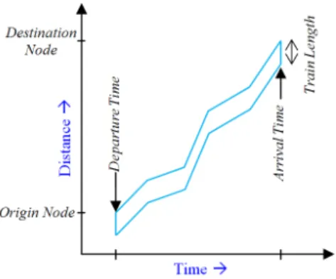
The railway track occupancy by existing passenger and freight trains in the network is determined by the operational working timetable. The timetable includes the information about train travel times between different nodes (stations, terminals) and operational restrictions such as speed limits, planned maintenance of tracks in the network. The timetables are generally visualized with the help of travel graphs. The travel graph illustrates the path occupied by passenger and freight trains through all the important network locations over 24-hour period, days, or weeks. Fig. 1 illustrates the conceptual model of the travel graph, where Y-axis represents distances between different nodes and X-axis represents time taken by trains to travel.
Fig. 1. Travel graph used for visualising the train timetables.
Freight train trips are to be planned in the existing network (containing existing passenger and other freight trains) to deal with the ever increasing port import/export operations. There are several types of constraints under which the freight trains operate. Some of the major constraints can be classified into loading/unloading constraints at
2 Michal, Huynh, Shukla, Munoz, Barthelemy/ Transportation Research Procedia 00 (2017) 000–000
the freight distribution is carried by rail in Australia (BITRE, 2009). It is predicted that rail freight services will grow significantly to be more than double by 2030. This growth is mainly attributed to the expected mineral export growth (BITRE, 2009). Therefore, increasingly, importance is being placed on efficient use of existing railway assets for freight transport.
Organisations managing this growth continuously receive increasing volumes of orders from customers such as sea-port corporations, mining industries, and international customers. Infrastructure improvement plans by the government are proposed, but do not facilitate the immediate need for higher export volumes. In some Australian ports, local topography and proximity to large cities limit the allowable train set configurations, leaving little alternative but to schedule additional freight movements to meet demand volumes. As a result, train operators have to schedule and plan feasible freight train trips in the existing railway network, which are largely time consuming and complex due to presence of large amount of constraints and factors. Lack of decision support tools and overwhelming demands for rail operators to explore feasible options for planning new freight trips before implementation adds to operational risks in planning. Furthermore, the use of complex mathematical models and optimization methods for freight trip simulation are restricted. Hence, a decision support platform is required which can help train operators to simulate existing train network together with the functionalities to plan and add new freight train trips.
The railway network planning and scheduling has attracted wider community of researchers in operational research due to the challenges posed at the strategic, tactical, and operational levels. Range of operations research (OR) tools and methodologies are proposed in this area. Caprara et al. (2002) proposed an integer linear programming (ILP) formulation for solving the periodic timetabling problem. The review of literature on railroad planning and scheduling have been discussed in (Ahuja et al., 2005). Törnquist (2005) has reviewed the models and algorithms in railway traffic scheduling and dispatching with a focus on problem type, solution methodology, and experimental evaluation. Similarly, Cordeau et al., (1998) have reviewed various optimization models for train routing and scheduling. Recently, Mu and Dessouky (2011) and Cacchiani et al. (2010) have proposed optimisation approaches for scheduling freight trains in complex networks. Further, Confessore et al. (2009) have used simulation based methods for estimating capacity of railways. Although, these approaches are known to be useful to find an optimal and sub-optimal solutions for complex optimization problems in rail network planning and scheduling; this requires the decision makers to have good grasp in operations research based mathematical modelling and optimisation, which restricts their use in real situations. Furthermore, real life cases can involve several problem specific and system related constraints which are difficult to model in a closed form, making it infeasible to be implemented. Therefore, instead of developing complex optimisation methods for global optimal solution to the problem, a simulation model based method is proposed. The proposed simulation modelling platform can be used by decision makers having little OR and simulation background.
There are many simulation models developed for many years, which are used for analysis of both passenger rail systems and freight transport networks. Several types of models are developed for simulation to model railroad problems at varying geographic scales. Macro-level simulation models are developed for high-level network planning problems and cover large geographic area. Examples of these models include countrywide freight model in Spain (Garcia and Gutierrez, 2003), a regional freight model in Southern California (WGI 2007), and an intra-urban passenger/freight network in North Carolina (Leilich 1998). Other type of simulation models are known as micro-level models which generally focus on the operations aspects of a citywide rail networks (Nash et al. 2006) or at the yard and terminal level (Dalal and Jensen, 2001). These micro-level models concentrate mainly on train movements and their network operations.
The rail simulation model (called ‘RailNet’) we describe in this paper aims at providing a tool to assist train and rail network operators with long term planning, by allowing them to visualize the performance of the network and to carry out scheduling tasks. RailNet extracts the occupancy of existent trains (for both passenger and freight services) along a route across the rail network from a working timetable and plots them on a graph of track nodes on this route versus time. On such a graph, the occupancy of a train path sharing track segments with this route is represented by a polygon or a series of polygons in a 2-dimensional space. In order to enable RailNet to schedule additional train paths on this route, a space partitioning algorithm was developed to divide this 2-dimensional space into subsets of occupied space (i.e. the aforementioned polygons) and available space. RailNet then assesses the viability of subsets
Guillaume Michal et al. / Transportation Research Procedia 25 (2017) 461–473 463
Michal, Huynh, Shukla, Munoz, Barthelemy/ Transportation Research Procedia 00 (2017) 000–000 3
of available space as new paths, taking into account the train length, specified departure time and the window of arrival time.
RailNet can be used to simulate track network at both macro-level (e.g. urban or regional rail networks) and local level (e.g. track networks at coal fields, train unloading terminals at sea ports). It plans additional freight movements in and around existing freight paths and passenger paths while avoiding collisions and adhering to track segment speed limits. Thanks to this feature, it can assist commodity based industries to find additional capacity in existing infrastructure and operational configurations.
This paper is organised as follows. Section 2 discusses the problem of freight train trip planning in railway networks, with the focus being on the railway network in New South Wales (NSW), Australia. Section 3 discusses the simulation modelling platform RailNet which is can be used for automated trip planning and evaluation. Section 4 discusses a real case study in which RailNet was used to quantify the capacity of the track network at the Port Kembla Coal Terminal in NSW, Australia under different scenarios of infrastructure upgrades. The paper is concluded in Section 5.
2. Problem statement
Sea ports are the main entry and exit points for variety of freights ranging from bulk materials (such as coal, ores, and crude oil) to non-bulk items (such as vehicles). Port corporations face challenges related to planning and scheduling rail operations. Largely, these rail operations include planning and scheduling freight rail movements on a network of railway tracks shared with passenger trains and other freight trains. The number of operational complexities present significant trade-offs in volumes occurring on a regular basis. These complexities include fleet availability and reliability, load point constraints, and refueling delays. Amongst these complexities there is a clear necessity to schedule additional freight movements to meet the increasing demands of international customers. The total demand volumes must be met within operational and network constraints, leaving operators with little recourse but to attempt to plan more freight train movements to account for exogenous operational uncertainties.
The railway track occupancy by existing passenger and freight trains in the network is determined by the operational working timetable. The timetable includes the information about train travel times between different nodes (stations, terminals) and operational restrictions such as speed limits, planned maintenance of tracks in the network. The timetables are generally visualized with the help of travel graphs. The travel graph illustrates the path occupied by passenger and freight trains through all the important network locations over 24-hour period, days, or weeks. Fig. 1 illustrates the conceptual model of the travel graph, where Y-axis represents distances between different nodes and X-axis represents time taken by trains to travel.
Fig. 1. Travel graph used for visualising the train timetables.
Freight train trips are to be planned in the existing network (containing existing passenger and other freight trains) to deal with the ever increasing port import/export operations. There are several types of constraints under which the freight trains operate. Some of the major constraints can be classified into loading/unloading constraints at
2 Michal, Huynh, Shukla, Munoz, Barthelemy/ Transportation Research Procedia 00 (2017) 000–000
the freight distribution is carried by rail in Australia (BITRE, 2009). It is predicted that rail freight services will grow significantly to be more than double by 2030. This growth is mainly attributed to the expected mineral export growth (BITRE, 2009). Therefore, increasingly, importance is being placed on efficient use of existing railway assets for freight transport.
Organisations managing this growth continuously receive increasing volumes of orders from customers such as sea-port corporations, mining industries, and international customers. Infrastructure improvement plans by the government are proposed, but do not facilitate the immediate need for higher export volumes. In some Australian ports, local topography and proximity to large cities limit the allowable train set configurations, leaving little alternative but to schedule additional freight movements to meet demand volumes. As a result, train operators have to schedule and plan feasible freight train trips in the existing railway network, which are largely time consuming and complex due to presence of large amount of constraints and factors. Lack of decision support tools and overwhelming demands for rail operators to explore feasible options for planning new freight trips before implementation adds to operational risks in planning. Furthermore, the use of complex mathematical models and optimization methods for freight trip simulation are restricted. Hence, a decision support platform is required which can help train operators to simulate existing train network together with the functionalities to plan and add new freight train trips.
The railway network planning and scheduling has attracted wider community of researchers in operational research due to the challenges posed at the strategic, tactical, and operational levels. Range of operations research (OR) tools and methodologies are proposed in this area. Caprara et al. (2002) proposed an integer linear programming (ILP) formulation for solving the periodic timetabling problem. The review of literature on railroad planning and scheduling have been discussed in (Ahuja et al., 2005). Törnquist (2005) has reviewed the models and algorithms in railway traffic scheduling and dispatching with a focus on problem type, solution methodology, and experimental evaluation. Similarly, Cordeau et al., (1998) have reviewed various optimization models for train routing and scheduling. Recently, Mu and Dessouky (2011) and Cacchiani et al. (2010) have proposed optimisation approaches for scheduling freight trains in complex networks. Further, Confessore et al. (2009) have used simulation based methods for estimating capacity of railways. Although, these approaches are known to be useful to find an optimal and sub-optimal solutions for complex optimization problems in rail network planning and scheduling; this requires the decision makers to have good grasp in operations research based mathematical modelling and optimisation, which restricts their use in real situations. Furthermore, real life cases can involve several problem specific and system related constraints which are difficult to model in a closed form, making it infeasible to be implemented. Therefore, instead of developing complex optimisation methods for global optimal solution to the problem, a simulation model based method is proposed. The proposed simulation modelling platform can be used by decision makers having little OR and simulation background.
There are many simulation models developed for many years, which are used for analysis of both passenger rail systems and freight transport networks. Several types of models are developed for simulation to model railroad problems at varying geographic scales. Macro-level simulation models are developed for high-level network planning problems and cover large geographic area. Examples of these models include countrywide freight model in Spain (Garcia and Gutierrez, 2003), a regional freight model in Southern California (WGI 2007), and an intra-urban passenger/freight network in North Carolina (Leilich 1998). Other type of simulation models are known as micro-level models which generally focus on the operations aspects of a citywide rail networks (Nash et al. 2006) or at the yard and terminal level (Dalal and Jensen, 2001). These micro-level models concentrate mainly on train movements and their network operations.
The rail simulation model (called ‘RailNet’) we describe in this paper aims at providing a tool to assist train and rail network operators with long term planning, by allowing them to visualize the performance of the network and to carry out scheduling tasks. RailNet extracts the occupancy of existent trains (for both passenger and freight services) along a route across the rail network from a working timetable and plots them on a graph of track nodes on this route versus time. On such a graph, the occupancy of a train path sharing track segments with this route is represented by a polygon or a series of polygons in a 2-dimensional space. In order to enable RailNet to schedule additional train paths on this route, a space partitioning algorithm was developed to divide this 2-dimensional space into subsets of occupied space (i.e. the aforementioned polygons) and available space. RailNet then assesses the viability of subsets
464 Guillaume Michal et al. / Transportation Research Procedia 25 (2017) 461–473 Michal, Huynh, Shukla, Munoz, Barthelemy/ Transportation Research Procedia 00 (2017) 000–000 5 3.1.2 Track nodes
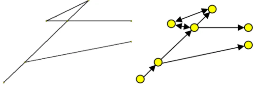
These entities represent junctions, stations, location of signal boxes, railroad switch, and ends of track segments across the rail network. Fig. 2a illustrates a section of railway network with nodes and various track segments connecting them. Stations are the locations in the track network where trains can park, stop or pass through. Trains can overtake and cross at stations having multiple track. Junctions are locations where two different track segments fork. The information about stations, junctions, segment ends, and their locations are generally available with the track infrastructure managers. In digraph G, it is represented as v1∈ V, which ordered set of nodes on the track network.
Fig. 2. (a) Section of the railway network having nodes and track segments; (b) corresponding digraph with nodes and directed edges. 3.1.3 Trains
These are the entities in the model which are free to move on the track segments to traverse from their origin node to destination node in the network. T is defined as finite set of trains which are considered in this model.
T = {t+, t,, t-, … , tL} (4)
T = TN∪ TPQR and TN∩ TPQR= ∅ (5)
In Equation 5 TN⊂ T is a subset of existing trains that are currently running in the network and whose timetable cannot be modified. TPQR⊆ T is a subset of trains that new freight trains which are not scheduled and therefore, does not have any timetable yet. So the problem is to assign feasible timetable and path to each trains in TPQR by following this conceptual modelling framework.
For each train t ∈ T, there is an ordered set of nodes defined by VW which represents the journey of tWX train. VW represents the order of nodes that is used by tWX train in the network, mathematically expressed as below
VW= v+W, v,W, v-W, … , vPWY ∀t ∈ T, ∃VW: VW⊆ V (6)
In Equation 6 v1W and vPWY represents the iWX and last node traversed by train t, respectively.
Further, each train t ∈ T will have set of arrival (AW∀t ∈ T) and departure times (DW∀t ∈ T) to and from nodes in VW.
AW= (a]W^, a]W_, … , a]W`, … , aW](|bY|c^)) , where v1 ∈ VW\{vPWY} (7)
DW= (d]W^, d]W_, … , dW]`, … , d]W(|bY|c^)) , where v1 ∈ VW\{veW} (8)
In Equations 7 and 8, a]W` and d]W` represents the arrival and departure times for the tWX train at v1W.
Let us consider, θ]W`→]`g^ be the time taken by tWX train to travel from node v1W to v1h+W . This can be evaluated by
using maximum allowable speed on the track segment connecting v1W and v1h+W and length of the track segment
4 Michal, Huynh, Shukla, Munoz, Barthelemy/ Transportation Research Procedia 00 (2017) 000–000
nodes, track lengths, track occupancy constraints, planned maintenance or closure of nodes and tracks, refueling/crew change constraints, collision constraint, and allowable staging of trains on rail tracks.
Movement of freights to and from ports through freight trains is contingent upon their adherence to abovementioned constraints and available time windows in the existing rail network, without causing significant time delays. Excessive time delays associated with the freight trains may impact the movements of other trains and can result in widespread delays across the whole network. Thus, planning and scheduling of the freight train trips to and from ports becomes a complex task for freight train operators. Therefore, a computational modelling platform is required for them to understand the current or existing rail network traffic, consisting of passenger trains and other freight trains, and schedule/plan new freight train trips. The model will also help freight train operators to oversee the railway traffic for bottleneck assessments and streamline rail freight operations. The next section discusses the modelling platform developed for simulating the existing network and for performing experiments to fit new freight train trips.
3. RailNet: a modelling platform for freight train operations
This section details the modelling platform RailNet that simulates the operation of train services on an existing railway network with and more importantly allows for the scheduling of new (freight) train trips.
3.1. Conceptual model of a rail network
In this section, the conceptual representation of a rail network infrastructure is discussed. This infrastructure representation describes the type of railway infrastructure that the approach can be applied to. The rail network can be defined as a digraph, which are graphs having directed edges between source and target nodes. Let us define digraph ≔ (V, E, s, f) , where V = (v+, v,, v-, … v/) is a set of nodes (i.e. track nodes), E = (e+, e,, e-, … ) is a set of edges (i.e. track segments), and s and f define the function which maps e1 to its source and target node. Mathematically these functions are defined by Equation 1.
𝑠𝑠, 𝑓𝑓: 𝐸𝐸 → 𝑉𝑉 (1)
The description about the relationships between G and rail network are discussed below.
3.1.1 Track segments
These are the stationary entities within the model which maps the railway tracks or routes. In digraph G, it is represented as e1∈ E. Fig. 2a illustrates the track segments in a rail network. Fig. 2b illustrates corresponding digraph with nodes and directed edges. Further, each e1 ∈ E has the speed limit constraint (defined by function sp: E → SL) which limits the train movements on e1. Where, SL is a set of speed limits (sl+, sl,, sl-, … ). The track segment attributes such as track length, availability for staging, and others can be associated with each e1∈ E such that
e1= l1, stage1 , ∀ e1∈ E (2)
stage1= 10 if staging is not allowedif staging is allowed (3) In Equation 2, l1 represents the length of the track segment and stage1 is the decision variable which defines whether or not staging is allowed on e1. The directionality of track segments are included in the model using functions s and f. These functions can define the track segment to be either uni-directional or bi-directional.
Guillaume Michal et al. / Transportation Research Procedia 25 (2017) 461–473 465
Michal, Huynh, Shukla, Munoz, Barthelemy/ Transportation Research Procedia 00 (2017) 000–000 5 3.1.2 Track nodes
These entities represent junctions, stations, location of signal boxes, railroad switch, and ends of track segments across the rail network. Fig. 2a illustrates a section of railway network with nodes and various track segments connecting them. Stations are the locations in the track network where trains can park, stop or pass through. Trains can overtake and cross at stations having multiple track. Junctions are locations where two different track segments fork. The information about stations, junctions, segment ends, and their locations are generally available with the track infrastructure managers. In digraph G, it is represented as v1∈ V, which ordered set of nodes on the track network.
Fig. 2. (a) Section of the railway network having nodes and track segments; (b) corresponding digraph with nodes and directed edges. 3.1.3 Trains
These are the entities in the model which are free to move on the track segments to traverse from their origin node to destination node in the network. T is defined as finite set of trains which are considered in this model.
T = {t+, t,, t-, … , tL} (4)
T = TN∪ TPQR and TN∩ TPQR= ∅ (5)
In Equation 5 TN⊂ T is a subset of existing trains that are currently running in the network and whose timetable cannot be modified. TPQR ⊆ T is a subset of trains that new freight trains which are not scheduled and therefore, does not have any timetable yet. So the problem is to assign feasible timetable and path to each trains in TPQR by following this conceptual modelling framework.
For each train t ∈ T, there is an ordered set of nodes defined by VW which represents the journey of tWX train. VW represents the order of nodes that is used by tWX train in the network, mathematically expressed as below
VW= v+W, v,W, vW-, … , vPWY ∀t ∈ T, ∃VW: VW⊆ V (6)
In Equation 6 v1W and vPWY represents the iWX and last node traversed by train t, respectively.
Further, each train t ∈ T will have set of arrival (AW∀t ∈ T) and departure times (DW∀t ∈ T) to and from nodes in VW.
AW= (aW]^, a]W_, … , a]W`, … , a]W(|bY|c^)) , where v1∈ VW\{vPWY} (7)
DW= (d]W^, d]W_, … , dW]`, … , d]W(|bY|c^)) , where v1∈ VW\{veW} (8)
In Equations 7 and 8, a]W` and d]W` represents the arrival and departure times for the tWX train at v1W.
Let us consider, θ]W`→]`g^ be the time taken by tWX train to travel from node v1W to v1h+W . This can be evaluated by
using maximum allowable speed on the track segment connecting v1W and v1h+W and length of the track segment
4 Michal, Huynh, Shukla, Munoz, Barthelemy/ Transportation Research Procedia 00 (2017) 000–000
nodes, track lengths, track occupancy constraints, planned maintenance or closure of nodes and tracks, refueling/crew change constraints, collision constraint, and allowable staging of trains on rail tracks.
Movement of freights to and from ports through freight trains is contingent upon their adherence to abovementioned constraints and available time windows in the existing rail network, without causing significant time delays. Excessive time delays associated with the freight trains may impact the movements of other trains and can result in widespread delays across the whole network. Thus, planning and scheduling of the freight train trips to and from ports becomes a complex task for freight train operators. Therefore, a computational modelling platform is required for them to understand the current or existing rail network traffic, consisting of passenger trains and other freight trains, and schedule/plan new freight train trips. The model will also help freight train operators to oversee the railway traffic for bottleneck assessments and streamline rail freight operations. The next section discusses the modelling platform developed for simulating the existing network and for performing experiments to fit new freight train trips.
3. RailNet: a modelling platform for freight train operations
This section details the modelling platform RailNet that simulates the operation of train services on an existing railway network with and more importantly allows for the scheduling of new (freight) train trips.
3.1. Conceptual model of a rail network
In this section, the conceptual representation of a rail network infrastructure is discussed. This infrastructure representation describes the type of railway infrastructure that the approach can be applied to. The rail network can be defined as a digraph, which are graphs having directed edges between source and target nodes. Let us define digraph ≔ (V, E, s, f) , where V = (v+, v,, v-, … v/) is a set of nodes (i.e. track nodes), E = (e+, e,, e-, … ) is a set of edges (i.e. track segments), and s and f define the function which maps e1 to its source and target node. Mathematically these functions are defined by Equation 1.
𝑠𝑠, 𝑓𝑓: 𝐸𝐸 → 𝑉𝑉 (1)
The description about the relationships between G and rail network are discussed below.
3.1.1 Track segments
These are the stationary entities within the model which maps the railway tracks or routes. In digraph G, it is represented as e1∈ E. Fig. 2a illustrates the track segments in a rail network. Fig. 2b illustrates corresponding digraph with nodes and directed edges. Further, each e1∈ E has the speed limit constraint (defined by function sp: E → SL) which limits the train movements on e1. Where, SL is a set of speed limits (sl+, sl,, sl-, … ). The track segment attributes such as track length, availability for staging, and others can be associated with each e1∈ E such that
e1 = l1, stage1 , ∀ e1 ∈ E (2)
stage1= 10 if staging is not allowedif staging is allowed (3) In Equation 2, l1 represents the length of the track segment and stage1 is the decision variable which defines whether or not staging is allowed on e1. The directionality of track segments are included in the model using functions s and f. These functions can define the track segment to be either uni-directional or bi-directional.
466 Guillaume Michal et al. / Transportation Research Procedia 25 (2017) 461–473 Michal, Huynh, Shukla, Munoz, Barthelemy/ Transportation Research Procedia 00 (2017) 000–000 7
d]W`− aW]`≥ γ1W (15)
Delay due braking and speeding for unexpected stops. Speeding and braking time will have to be added to
normal time θ]W`→]`g^ between v1 and v1h+ when a trains stops unexpectedly (due to crossing and overtaking) at
station where γ1W= 0. Let the additional time be represented as τW. Thus,
dW]`− aW]`> 0 ∧ γW1 = 0 ⇒ θW]`c^→]` = θW]`c^→]`+ τW θ]W`→]`g^= θ]W`→]`g^− τW (16)
Buffer time. There is a minimum buffer time (µ1) allowed between the departure times of two trains (tL, tt) travelling on same track (eL which directs from v1 to v1h+) and in same direction.
d]`
Wu− d
]`
Ww
Qu≥ µ1 (17)
Maximum allowed staging. There is a constraint which restricts the amount of time that any train t ∈ TPQR can stage on track eL which directs from v1 to v1h+. Staging time at the busy track segments can be less or zero compared to the less busy segments. Let us consider, φL be the maximal staging time on eL. Thus,
aW]`g^− d]W` Qu≤ φL ⋀ stageL= 1 (18)
3.2.3 Infrastructure related constraints
Track curfew. This constraint restricts the movement of trains t ∈ TPQR on tracks eL which directs from v1 to v1h+ at the maintenance time interval [CkQu, C
lQu]. Thus, d]W` Qu< Ck Qu ⋀ a ]` W Qu< Ck Qu (19)
Using the abovementioned constraints, new freight train trips can be planned such that it satisfies all the constraints. This will require various complex computations and interactions to be computed for each freight train. The functionalities of RailNet help freight train operators to plan new train trips without having to tackle these complex interactions manually.
3.3. RailNet simulation model
As described in the previous section, RailNet makes use of a combination of rail line components that include nodes, track segments with its attributes, and train timetables for all the running services, including passenger trains, freight trains, and trains for maintenance purposes. The model features a friendly user graphical interface that the user can interact with to perform operating/management tasks such as planning new freight train paths, or viewing network statistics and performance. Next subsection illustrates the steps involved and functionalities present in the current RailNet simulation platform for new freight trip planning.
3.3.1 Data input and network generation
Remove inconsistencies in working timetable. The rail network generation function starts with inputting the
network related data by removing the inconsistencies in the existing working timetables. This function checks for errors in the working timetable provided by train operating organisations so that it can be used in RailNet model. The rail network is populated with currently running passenger and/or freight trains working timetable in comma
6 Michal, Huynh, Shukla, Munoz, Barthelemy/ Transportation Research Procedia 00 (2017) 000–000
(defined in section 3.1.1). Existing freight and passenger trains movements are modelled as the time periods (determined by AW to DW) when sets of track segments are unavailable.
Other train related attributes such as train lengths, commodity, and train capacity can be also included in this model but for the sake of brevity these are not considered in this study.
3.2. New freight train trip planning
The problem addressed in this paper is to insert new train trips into the existing timetable for freight trains. The new set of freight trains to be inserted in the current timetable is represented as TPQR. Each train t ∈ TPQR will have a origin node (defined as viW ∈ V), destination node (vPWY∈ V), time window for departure from viW and arrival at vPWY.
Let the departure time window from viW be αkW, αlW and arrival time window at vWPY be βkW, βlW . There are various
constraints based on the freight train operator requirements, operational constraints, and infrastructure related constraints. These constraints are mathematically modelled as described below.
3.2.1 Operator requirements
Origin departure. Each train t ∈ TPQR should depart from origin node viW ∈ V such that,
αkW ≤ d]Wo≤ αlW (9)
Destination arrival. Each train t ∈ TPQR should arrive at destination node vPWY∈ V such that,
βkW ≤ a]WpY ≤ βlW (10)
Maximum allowable delay in trip completion. Let a maximum allowable trip completion time be defined as φW and the minimum trip time, which is defined for each train, be MW. Thus this constraint is defined as
aW]pY− d]Wo− MW≤ φW (11)
3.2.2 Operational constraints
Running time. The running time for train t on the network should satisfy following constraint
aW]`g^− d]W` = θ]W`→]`g^ (12)
Overtaking. This constraint will avoid trains tL, tt ⊆ TPQR, travelling in the same directions on a same track segment between v1 and v1h+ in their journeys. This is modelled as
a]`g^ Wu > a ]`g^ Ww ↔ d ]` Wu> d ]` Ww (13)
Crossing. This constraint will avoid trains tL, tt traveling in opposite direction on a same track segment between v1 and v1h+ in their journeys. This is modeled as
d]`g^ Wu > a ]`g^ Ww ∨ d ]` Ww > a ]` Wu (14)
Train stopping at stations. A train t ∈ TPQR, has to stop at station/node v1W for at least γ1W time units. Where γ1W is the amount of time units that train t has to stop at v1W. The value of γ1W for freight trains is normally computed based on the loading/unloading capacity at particular stations. Mathematically,
Guillaume Michal et al. / Transportation Research Procedia 25 (2017) 461–473 467
Michal, Huynh, Shukla, Munoz, Barthelemy/ Transportation Research Procedia 00 (2017) 000–000 7
d]W`− a]W` ≥ γ1W (15)
Delay due braking and speeding for unexpected stops. Speeding and braking time will have to be added to
normal time θ]W`→]`g^ between v1 and v1h+ when a trains stops unexpectedly (due to crossing and overtaking) at
station where γ1W= 0. Let the additional time be represented as τW. Thus,
dW]`− a]W` > 0 ∧ γW1 = 0 ⇒ θW]`c^→]`= θW]`c^→]`+ τW θ]W`→]`g^ = θ]W`→]`g^− τW (16)
Buffer time. There is a minimum buffer time (µ1) allowed between the departure times of two trains (tL, tt) travelling on same track (eL which directs from v1 to v1h+) and in same direction.
d]`
Wu− d
]`
Ww
Qu≥ µ1 (17)
Maximum allowed staging. There is a constraint which restricts the amount of time that any train t ∈ TPQR can stage on track eL which directs from v1 to v1h+. Staging time at the busy track segments can be less or zero compared to the less busy segments. Let us consider, φL be the maximal staging time on eL. Thus,
a]W`g^− d]W` Qu≤ φL ⋀ stageL= 1 (18)
3.2.3 Infrastructure related constraints
Track curfew. This constraint restricts the movement of trains t ∈ TPQR on tracks eL which directs from v1 to v1h+ at the maintenance time interval [CkQu, C
l Qu]. Thus, d]W` Qu< Ck Qu ⋀ a ]` W Qu< Ck Qu (19)
Using the abovementioned constraints, new freight train trips can be planned such that it satisfies all the constraints. This will require various complex computations and interactions to be computed for each freight train. The functionalities of RailNet help freight train operators to plan new train trips without having to tackle these complex interactions manually.
3.3. RailNet simulation model
As described in the previous section, RailNet makes use of a combination of rail line components that include nodes, track segments with its attributes, and train timetables for all the running services, including passenger trains, freight trains, and trains for maintenance purposes. The model features a friendly user graphical interface that the user can interact with to perform operating/management tasks such as planning new freight train paths, or viewing network statistics and performance. Next subsection illustrates the steps involved and functionalities present in the current RailNet simulation platform for new freight trip planning.
3.3.1 Data input and network generation
Remove inconsistencies in working timetable. The rail network generation function starts with inputting the
network related data by removing the inconsistencies in the existing working timetables. This function checks for errors in the working timetable provided by train operating organisations so that it can be used in RailNet model. The rail network is populated with currently running passenger and/or freight trains working timetable in comma
6 Michal, Huynh, Shukla, Munoz, Barthelemy/ Transportation Research Procedia 00 (2017) 000–000
(defined in section 3.1.1). Existing freight and passenger trains movements are modelled as the time periods (determined by AW to DW) when sets of track segments are unavailable.
Other train related attributes such as train lengths, commodity, and train capacity can be also included in this model but for the sake of brevity these are not considered in this study.
3.2. New freight train trip planning
The problem addressed in this paper is to insert new train trips into the existing timetable for freight trains. The new set of freight trains to be inserted in the current timetable is represented as TPQR. Each train t ∈ TPQR will have a origin node (defined as viW ∈ V), destination node (vPWY∈ V), time window for departure from viW and arrival at vPWY.
Let the departure time window from viW be αkW, αlW and arrival time window at vPWY be βkW, βlW . There are various
constraints based on the freight train operator requirements, operational constraints, and infrastructure related constraints. These constraints are mathematically modelled as described below.
3.2.1 Operator requirements
Origin departure. Each train t ∈ TPQR should depart from origin node viW ∈ V such that,
αkW ≤ d]Wo≤ αlW (9)
Destination arrival. Each train t ∈ TPQR should arrive at destination node vPWY∈ V such that,
βkW ≤ a]WpY ≤ βlW (10)
Maximum allowable delay in trip completion. Let a maximum allowable trip completion time be defined as φW and the minimum trip time, which is defined for each train, be MW. Thus this constraint is defined as
a]WpY− d]Wo− MW≤ φW (11)
3.2.2 Operational constraints
Running time. The running time for train t on the network should satisfy following constraint
a]W`g^− d]W`= θ]W`→]`g^ (12)
Overtaking. This constraint will avoid trains tL, tt ⊆ TPQR, travelling in the same directions on a same track segment between v1 and v1h+ in their journeys. This is modelled as
a]`g^ Wu > a ]`g^ Ww ↔ d ]` Wu> d ]` Ww (13)
Crossing. This constraint will avoid trains tL, tt traveling in opposite direction on a same track segment between v1 and v1h+ in their journeys. This is modeled as
d]`g^ Wu > a ]`g^ Ww ∨ d ]` Ww > a ]` Wu (14)
Train stopping at stations. A train t ∈ TPQR, has to stop at station/node v1W for at least γ1W time units. Where γ1W is the amount of time units that train t has to stop at v1W. The value of γ1W for freight trains is normally computed based on the loading/unloading capacity at particular stations. Mathematically,
468 Guillaume Michal et al. / Transportation Research Procedia 25 (2017) 461–473 Michal, Huynh, Shukla, Munoz, Barthelemy/ Transportation Research Procedia 00 (2017) 000–000 9
In order to plan new train trips – a particular train type t is selected from the list of trains TPQR; their origin to destination trip is selected from the list of trips VW; earliest departure time of new train trip at origin; arrival time window at destination βkW, βlW ; and, maximum allowable time for arrival at the destination node φW. Users can select each of these parameters from the user interface and the feasibility of these trips can be analysed. The simulation model analyses the feasibility of the new train trip paths given abovementioned parameters based on model defined in Section 3.2.
Fig. 3. RailNet interface for new trip planning. 3.3.3 Visualisation and performance measurement
This section details various types of analysis and visualisation that can be performed using RailNet.
Fig. 4. Calendar table listing all the train trips (existing and newly scheduled) 8 Michal, Huynh, Shukla, Munoz, Barthelemy/ Transportation Research Procedia 00 (2017) 000–000
separated value (.csv) format. The model checks the timetable for a certain errors (for example inconsistency in data format) and removes them if there are any to make sure the currently working timetable is feasible/suitable for simulation.
Generate local networks. This function helps to create various separate railway networks such as port network,
colliery network, passenger train network; which are separately managed by different train operating organisations. Options of format of input data which can be used to create a local network are described below.
• Working timetable: this is a modified version of working timetable obtained from section 3.3.1.1. This helps to determine AW, DW ∀t ∈ TN.
• Network spreadsheets: information of the network can alternatively be stored in two spreadsheets (or CSV files). One contains data of network nodes (V), and the other contains data of track segments (E).
• Trip templates: A trip template is defined as a sequence of nodes and sections a train can take to travel from a particular origin to destination node (i.e., VW). Most of the time, train operating organisations use these templates for managing their train movements in the network.
Generate a global network. This function combines and re-indexes nodes and sections that are present in multiple
local networks created in section 3.3.1.2 to form a global network.
Identify routes for new freight trains. This function identifies routes or templates (VW) for each trains that can planned (TPQR) from working timetable. It extracts list of sequence of nodes that belong to each trains that will be used for planning. This is done because most trains have pre-defined set of routes (sequences of network nodes) which they can take while running between a particular origin and destination node. Therefore, the new freight trains will use these templates for planning trips in next subsection.
3.3.2 Planning trips for new freight trains
This subsection will use the global network created in section 3.3.1.3 and list of trains with their templates that will be used for planning. Users or train operators can select few freight trains from the comprehensive list of trains to be planned (TPQR). Then following files/data are used for setting parameters for planning new freight train trips. • Select a list of rules, which is a csv file, of user-specified track unavailability, i.e. [CkQu, C
lQu].
• Select a dwelling file, which contains user-defined information of track nodes where trains can stop and sections where trains can stage, i.e. stage1.
• Select a starting date and end date for the simulation period (the ‘calendar’)
• Enter a time buffer between trains in seconds which applies to all trains, i.e. same buffer time applies between two freight trains, two passenger trains or between a freight train and a passenger train, i.e., µ1.
• More information about special nodes such as refueling nodes and nodes where coal/grain unloaders are located can be also inputted. However, these are not detailed in this paper for the sake of brevity.
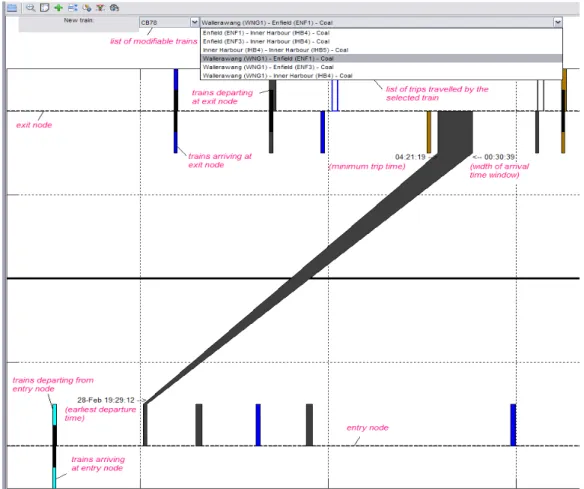
The RailNet layout for planning new freight train trips is illustrated in Fig. 3. Elements of the trip management layout shown in Fig. 3 includes
• a list of trains that can be used for planning new trips, i.e., TPQR
• a list of trips (origin to destination, i.e., viW and vPWY) travelled by each train t ∈ TPQR
• two bold horizontal dashed lines represents the origin node (the lower line) and destination node (the upper line) of the selected trip in distance time graph
• vertical bars above and below the bold horizontal dashed lines represents the incoming and outgoing trips. These bars are coloured based on the commodity a particular train is carrying. The width of each vertical bar represents the time duration that a corresponding train occupies at the origin or destination node.
Guillaume Michal et al. / Transportation Research Procedia 25 (2017) 461–473 469
Michal, Huynh, Shukla, Munoz, Barthelemy/ Transportation Research Procedia 00 (2017) 000–000 9
In order to plan new train trips – a particular train type t is selected from the list of trains TPQR; their origin to destination trip is selected from the list of trips VW; earliest departure time of new train trip at origin; arrival time window at destination βkW, βlW ; and, maximum allowable time for arrival at the destination node φW. Users can select each of these parameters from the user interface and the feasibility of these trips can be analysed. The simulation model analyses the feasibility of the new train trip paths given abovementioned parameters based on model defined in Section 3.2.
Fig. 3. RailNet interface for new trip planning. 3.3.3 Visualisation and performance measurement
This section details various types of analysis and visualisation that can be performed using RailNet.
Fig. 4. Calendar table listing all the train trips (existing and newly scheduled) 8 Michal, Huynh, Shukla, Munoz, Barthelemy/ Transportation Research Procedia 00 (2017) 000–000
separated value (.csv) format. The model checks the timetable for a certain errors (for example inconsistency in data format) and removes them if there are any to make sure the currently working timetable is feasible/suitable for simulation.
Generate local networks. This function helps to create various separate railway networks such as port network,
colliery network, passenger train network; which are separately managed by different train operating organisations. Options of format of input data which can be used to create a local network are described below.
• Working timetable: this is a modified version of working timetable obtained from section 3.3.1.1. This helps to determine AW, DW ∀t ∈ TN.
• Network spreadsheets: information of the network can alternatively be stored in two spreadsheets (or CSV files). One contains data of network nodes (V), and the other contains data of track segments (E).
• Trip templates: A trip template is defined as a sequence of nodes and sections a train can take to travel from a particular origin to destination node (i.e., VW). Most of the time, train operating organisations use these templates for managing their train movements in the network.
Generate a global network. This function combines and re-indexes nodes and sections that are present in multiple
local networks created in section 3.3.1.2 to form a global network.
Identify routes for new freight trains. This function identifies routes or templates (VW) for each trains that can planned (TPQR) from working timetable. It extracts list of sequence of nodes that belong to each trains that will be used for planning. This is done because most trains have pre-defined set of routes (sequences of network nodes) which they can take while running between a particular origin and destination node. Therefore, the new freight trains will use these templates for planning trips in next subsection.
3.3.2 Planning trips for new freight trains
This subsection will use the global network created in section 3.3.1.3 and list of trains with their templates that will be used for planning. Users or train operators can select few freight trains from the comprehensive list of trains to be planned (TPQR). Then following files/data are used for setting parameters for planning new freight train trips. • Select a list of rules, which is a csv file, of user-specified track unavailability, i.e. [CkQu, C
l Qu].
• Select a dwelling file, which contains user-defined information of track nodes where trains can stop and sections where trains can stage, i.e. stage1.
• Select a starting date and end date for the simulation period (the ‘calendar’)
• Enter a time buffer between trains in seconds which applies to all trains, i.e. same buffer time applies between two freight trains, two passenger trains or between a freight train and a passenger train, i.e., µ1.
• More information about special nodes such as refueling nodes and nodes where coal/grain unloaders are located can be also inputted. However, these are not detailed in this paper for the sake of brevity.
The RailNet layout for planning new freight train trips is illustrated in Fig. 3. Elements of the trip management layout shown in Fig. 3 includes
• a list of trains that can be used for planning new trips, i.e., TPQR
• a list of trips (origin to destination, i.e., viW and vPWY) travelled by each train t ∈ TPQR
• two bold horizontal dashed lines represents the origin node (the lower line) and destination node (the upper line) of the selected trip in distance time graph
• vertical bars above and below the bold horizontal dashed lines represents the incoming and outgoing trips. These bars are coloured based on the commodity a particular train is carrying. The width of each vertical bar represents the time duration that a corresponding train occupies at the origin or destination node.
470 Guillaume Michal et al. / Transportation Research Procedia 25 (2017) 461–473
Michal, Huynh, Shukla, Munoz, Barthelemy/ Transportation Research Procedia 00 (2017) 000–000 11
Fig. 7. A snapshot of the network statistics
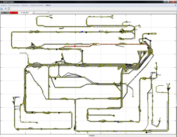
Generate network graph. This generates graph which shows the dynamics of trains as they move on the network
(see Fig. 6). Static yellow dots are network nodes in Fig. 6. Moving blue dots are the trains that can be used for planning new trips. Moving black dots are other trains (which cannot be used for planning new trips). The moving red dot is the activated train. The rail segments in red indicate the path of the activated train. Further, more information about each of the track segment and node can be obtained by clicking on them in the interface.
Analyse network statistics. This function shows the dynamic changes of nodal statistics on the network graph (see
Fig. 7). Users can select different statistics such as: nodal occupancy, nodal flow, nodal performance, and nodal congestion. In Fig. 7, green nodes represent lower nodal flow and red nodes represent high nodal flow.
4. Case study
The RailNet modelling platform was used to simulate the operations of coal trains in a complex rail network within the Port Kembla Coal Terminal in NSW, Australia. The aim of the exercise was to quantify the operational capacity of the network under various scenarios of infrastructure upgrade.
The railway tracks considered in this modelling exercise involved a circular closed loop railway track, aka the Balloon Loop, which is part of the Coal Terminal (see Fig. 8) and rail corridors external to coal terminal shared between passenger and freight trains. Currently, the Balloon Loop has a single entry point, a single exit point, two coal arrival railroads, two grain arrival railroads, one coal unloader, one grain unloader, four coal exit railroads and two grain exit railroads. Grain arrival roads cannot be shared with coal trains and vice versa. The coal arrival roads are named NN48 and NN53. Both arrival roads have a dwelling length without collisions of 815 meters. The single coal unloader is capable of unloading X tons per hours. The operation of freight trains based on these existent infrastructure elements in the Coal Terminal forms the base case against which simulation results of other upgrade options will be compared. In later discussions, we refer to this base case as option 0.
10 Michal, Huynh, Shukla, Munoz, Barthelemy/ Transportation Research Procedia 00 (2017) 000–000
Generate calendar table. This shows the list of all trips existing in the working timetable as well as new train
trips that were successfully scheduled by the model (Fig. 4).
Generate travel graph. This function generates the travel graph (distance-time graphs) for the selected trains (see
Fig. 5). The horizontal axis indicates the time line from the beginning to the end of the calendar. The vertical axis indicates the sequence of nodes the activated train travels.
Fig. 5. Travel graph for multiple trains on distance-time axis
Guillaume Michal et al. / Transportation Research Procedia 25 (2017) 461–473 471
Michal, Huynh, Shukla, Munoz, Barthelemy/ Transportation Research Procedia 00 (2017) 000–000 11
Fig. 7. A snapshot of the network statistics
Generate network graph. This generates graph which shows the dynamics of trains as they move on the network
(see Fig. 6). Static yellow dots are network nodes in Fig. 6. Moving blue dots are the trains that can be used for planning new trips. Moving black dots are other trains (which cannot be used for planning new trips). The moving red dot is the activated train. The rail segments in red indicate the path of the activated train. Further, more information about each of the track segment and node can be obtained by clicking on them in the interface.
Analyse network statistics. This function shows the dynamic changes of nodal statistics on the network graph (see
Fig. 7). Users can select different statistics such as: nodal occupancy, nodal flow, nodal performance, and nodal congestion. In Fig. 7, green nodes represent lower nodal flow and red nodes represent high nodal flow.
4. Case study
The RailNet modelling platform was used to simulate the operations of coal trains in a complex rail network within the Port Kembla Coal Terminal in NSW, Australia. The aim of the exercise was to quantify the operational capacity of the network under various scenarios of infrastructure upgrade.
The railway tracks considered in this modelling exercise involved a circular closed loop railway track, aka the Balloon Loop, which is part of the Coal Terminal (see Fig. 8) and rail corridors external to coal terminal shared between passenger and freight trains. Currently, the Balloon Loop has a single entry point, a single exit point, two coal arrival railroads, two grain arrival railroads, one coal unloader, one grain unloader, four coal exit railroads and two grain exit railroads. Grain arrival roads cannot be shared with coal trains and vice versa. The coal arrival roads are named NN48 and NN53. Both arrival roads have a dwelling length without collisions of 815 meters. The single coal unloader is capable of unloading X tons per hours. The operation of freight trains based on these existent infrastructure elements in the Coal Terminal forms the base case against which simulation results of other upgrade options will be compared. In later discussions, we refer to this base case as option 0.
10 Michal, Huynh, Shukla, Munoz, Barthelemy/ Transportation Research Procedia 00 (2017) 000–000
Generate calendar table. This shows the list of all trips existing in the working timetable as well as new train
trips that were successfully scheduled by the model (Fig. 4).
Generate travel graph. This function generates the travel graph (distance-time graphs) for the selected trains (see
Fig. 5). The horizontal axis indicates the time line from the beginning to the end of the calendar. The vertical axis indicates the sequence of nodes the activated train travels.
Fig. 5. Travel graph for multiple trains on distance-time axis
472 Guillaume Michal et al. / Transportation Research Procedia 25 (2017) 461–473 Michal, Huynh, Shukla, Munoz, Barthelemy/ Transportation Research Procedia 00 (2017) 000–000 13
With these new infrastructural change options, the simulation model for option 0 is used to plan new freight train trips from different coal pits/mines arriving and departing from balloon loop to satisfy projected demand. Currently running freight trains from each of the coal pits in year 2011 is considered as the base case (option 0) and extra freight trains from coal pits are to be planned for a future year to satisfy the projected demand with infrastructure change options (options 1 and 2). The simulation results are illustrated with the help of travel graphs in Fig. 9. This figure shows the existing train trips currently running in balloon loop (option 0), and new train trips that are planned together with existing train trips for option 1 and option 2.
The whole journey of trains in travel graphs in Fig. 9 is not illustrated as above travel graph is created for a particular track and the trains are using multiple railway tracks for completing respective journeys. For the sake of brevity, only few options of infrastructural changes and few freight train trips from coal pits are considered in the case study. Due to the confidentiality agreements with the organizations involved, most of the information is anonymously provided and only higher level data is discussed.
5. Conclusions
This paper presents a simulation modelling platform RailNet for modelling complex rail networks and assessing the feasibility of additional freight paths in the network. The model can also be used to assess the impact of rail infrastructural changes. The RailNet simulation platform takes into account network restrictions from passenger trains and port operational capacity. The inbuilt graphical user interfaces can help users to perform various analysis related to speed profiling, throughput issues, bottleneck analysis, capacity evaluation, network statistics and performance evaluation, timetabling of the trains, and planning of new train trips between origin and destination. The future research on RailNet simulation platform will include simulation optimisation module for optimising the operational parameters of the network together with the sequence of new train trips.
References
Ahuja, R. K., Cunha, C. B., Sahin, G., 2005. Network Models in Railroad Planning and Scheduling. Tutorials in Operations Research, pp 54-101. Cacchiani, V., Caprara, A., Toth, P., 2010. Scheduling extra freight trains on railway networks. Transportation Research Part B: Methodological,
44(2), 215-231.
Caprara, A., Fischetti, M., Toth, P., 2002. Modelling and solving the train timetabling problem modelling. Operations Research, 50(5), 851-861. Confessore, G., Liotta, G., Cicini, P., Rondinone, F., De Luca, P., 2009. A simulation-based approach for estimating the commercial capacity of
railways. Winter Simulation Conference, Austin, Texas, pp. 2542-2552.
Cordeau, J. F., Paolo, T., Daniele, V., 1998. A survey of optimization models for train routing and scheduling. Transportation Science, 32(4), 380-404.
Dalal, M. A., Jensen., L.P., 2001. Simulation modeling at union pacific railroad, Proceedings of the 33rd Conference on Winter Simulation, Arlington, Virginia, pp. 1048-1055.
Discussion paper, National Land Freight Strategy. Infrastructure Australia. 2011.
Garcia, I., Gutierrez, G., 2003. A simulation model for strategic planning in rail freight transport systems. ITE Journal, 73 (9), 32-40. Information sheet 34, Road and rail freight: competitors or complements? Bureau of Infrastructure, Transport, and Regional Economics, 2009. Leilich, R.H., 1998. Application of simulation models in capacity constrained rail corridors. Proceedings of the 30th Conference on Winter
Simulation, Washington D.C. pp. 1125 – 1134.
Mu, S., Dessouky, M., 2011. Scheduling freight trains travelling on complex networks. Transportation Research Part B: Methodological, 45(7), 1103-1123.
Nash, A., Weidmann, U., Bollinger, S., Luethi, M., Buchmueller, S., 2006. Increasing schedule reliability on Zurich’s S-Bahn through computer analysis and simulation. In: Transportation Research Record: Journal of the Transportation Research Board, No. 1955, TRB, National Research Council, Washington, D.C., pp. 16–25.
Törnquist, J., 2005. Computer-based decision support for railway traffic scheduling and dispatching: A review of models and algorithms. ATMOS2005 (Algorithmic Methods and Models for Optimization of Railways), Palma de Mallorca, Spain.
Washington Group International, Inc. 2007. RTC simulations—LOSSAN north railroad capacity and performance analysis. LOSSAN Rail Corridor Agency and IBI Group.
12 Michal, Huynh, Shukla, Munoz, Barthelemy/ Transportation Research Procedia 00 (2017) 000–000
Fig. 8. The track network (the Balloon Loop) at the Port Kemble Coal Terminal (NSW, Australia) considered in this case study.
Fig. 9. Travel graphs for option 0, option 1, and option 2 illustrating newly scheduled train trips in the Balloon Loop.
The capacity additions of each of the alternative scenarios and its corresponding throughput values for the coal terminal need to be investigated and quantified. Following are few infrastructural change options that are simulated with the help of RailNet simulation platform to determine new feasible train paths across the Balloon Loop. The output of the simulation informs the terminal operators if a particular infrastructure upgrade option will achieve the required level of throughput in a year.
• Option 1 – Extending the existent coal arrival roads to 850 metres. The rail network is otherwise unchanged. • Option 2 – Doubling the existent unloading capacity. The whole rail network remains unchanged.