RESEARCH OUTPUTS / RÉSULTATS DE RECHERCHE
Author(s) - Auteur(s) :
Publication date - Date de publication :
Permanent link - Permalien :
Rights / License - Licence de droit d’auteur :
Bibliothèque Universitaire Moretus Plantin
Institutional Repository - Research Portal
Dépôt Institutionnel - Portail de la Recherche
researchportal.unamur.be
University of Namur
CASE Tool Support for Temporal Database Design
Detienne, Virginie; Hainaut, Jean-Luc
Published in:
Proc of the 20th Int. Conf. on Conceptual modeling - ER 2001
Publication date:
2001
Link to publication
Citation for pulished version (HARVARD):
Detienne, V & Hainaut, J-L 2001, CASE Tool Support for Temporal Database Design. in S Hideko, K Sushil & J Arne (eds), Proc of the 20th Int. Conf. on Conceptual modeling - ER 2001: 20th international conference on
conceptual modeling (ER 2001). vol. 2224, Springer, Berlin, pp. 208-224.
General rights
Copyright and moral rights for the publications made accessible in the public portal are retained by the authors and/or other copyright owners and it is a condition of accessing publications that users recognise and abide by the legal requirements associated with these rights. • Users may download and print one copy of any publication from the public portal for the purpose of private study or research. • You may not further distribute the material or use it for any profit-making activity or commercial gain
• You may freely distribute the URL identifying the publication in the public portal ?
Take down policy
If you believe that this document breaches copyright please contact us providing details, and we will remove access to the work immediately and investigate your claim.
Abstract. Current RDBMS technology provides little support for building
tempo-ral databases. The paper describes a methodology and a CASE tool that is to help practitioners develop correct and efficient relational data structures. The designer builds a temporal ERA schema that is validated by the tool, then converted into a temporal relational schema. This schema can be transformed into a pure relational schema according to various optimization strategies. Finally, the tool generates an active SQL-92 database that automatically maintain entity and relationship states. In addition, it generates a temporal ODBC driver that encapsulates complex tem-poral operators such as projection, join and aggregation through a small subset of TSQL2. This API allows programmers to develop complex temporal applications as easily as non temporal ones.
1
Introduction
A wide range of database applications manage time-varying data. Existing database technology currently provides little support for managing such data, and using conven-tional data models and query languages like SQL-92 to cope with such information is particularly difficult [12]. Developers of database applications can create only ad-hoc solutions that must be reinvented each time a new application is developed.
The scientific community has long been interested in this problem [9]. The research has focused on characterizing the semantics of temporal information and on providing expressive and efficient means to model, store and query temporal data.
A lot of those studies concerned temporal data models and query languages. Dozens of extended relational data models have been proposed [13], while about 40 temporal query languages have been defined, most with their own data model, the most complete certainly being TSQL2 [11]. However, it seems that neither standardization bodies nor DBMS editors are really willing to adopt these proposals, so that the problem of main-taining and querying temporal data in an easy and reliable way remains unsolved.
A handful of temporal DBMS prototypes have been proposed [1], [13]. Attention has been paid to performance issues because selection, join, aggregates and duplicates elim-ination (coalescing) require sophisticated and time consuming algorithms [2].
Several temporally enhanced Entity-Relationship (ER) models have been developed [6]. UML (Unified Modelling Language) also has been extended with temporal seman-tics and notation (TUML) [14].
Among those studies, few methodologies and tools support have been proposed for temporal database design.
About this paper
Like for conventional databases, a temporal database design methodology must lead to correct and efficient databases. However, the design of even modest ones can be fairly
CASE Tool Support for Temporal Database Design
Virginie Detienne, Jean-Luc Hainaut
Institut d’Informatique, University of Namur rue Grandgagnage, 21 - B-5000 Namur - Belgium
complex, hence the need for CASE tools, specially for generating the code of the data-base. This paper describes a simple methodology and a CASE tool that is to help practi-tioners develop temporal applications based on SQL-92 technology.
These results are part of the TimeStamp project whose the goal is to provide practi-tioners with practical tools (models, methods, CASE tools and API) to design, manage and exploit temporal databases through standard technologies, such as C, ODBC and SQL-92. Though the models and the languages used are more simple than those avail-able in the literature, the authors feel that they can help developers in mastering their temporal data.
Sections 2, 3 and 4 introduce the concepts of temporal conceptual, logical and phys-ical models for relational temporal databases that are specific to the TimeStamp approach. Section 5 describes the methodology for temporal database design, and pre-sents a CASE tool that automates the processes defined in the methodology.
2
A Temporal Conceptual Model
The database conceptual schema of an information system is the major document through which the user requirements about an application domain are translated into abstract information structures. When the evolution of the components of this applica-tion domain is a part of these requirements, this schema must include temporal aspects. This new dimension increases the complexity of the conceptual model, and makes it more difficult to use and to understand. To alleviate this drawback, we have chosen a simple and intuitive formalism that must improve the reliability of the analysis process. This model brings three advantages, which should be evaluated against its loss of expressive power. First, it has been considered easier to use by developers when the time dimension must be taken into account (for instance, temporal consistency through inher-itance mechanism is far from trivial). Secondly, the distance between a conceptual schema and its relational expression is narrower, a quality that is appreciated by pro-grammers. Thirdly, schema expressed in a richer model can be converted without loss into simpler structures through semantics-preserving transformations [8].
Though the concepts of temporal conceptual schemas have been specified for long in the literature, we will describe them very briefly [14], [6].
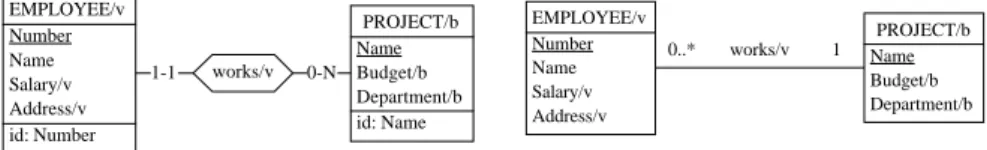
The conceptual model comprises three main constructs, namely entity types, single-valued atomic attributes and N-ary relationship types. Each construct can be non-tem-poral or temnon-tem-poral. In the first case, only the current states are of interest, while in the lat-ter case, we want to record past, current and future states. In this presentation, we will address the modelling and processing of historical states, that is the past and current states only1.
The temporal dimension can be based on valid time (/v), on transaction time (/t) or on both (/b for bitemporal). The instances of a non-temporal monotonic entity type (/m) can be created but never deleted, so that the letter enjoys some properties of temporal entity types. A construct is non-temporal, unless it is marked with a temporal tag: /m, /v,
1 Though most of the principles described in this paper can be extended to future states as well, the latter induce some constraints that we do not want to discuss in this paper. For instance, not all data distribution patterns proposed in the physical model can accommodate future states.
/t or /b (Fig. 1). An entity type can have one primary identifier (or key) and some sec-ondary identifiers. A relationship type has 2 or more roles, each of them being taken by an entity type. A role has a cardinality constraint defined by two numbers, the most com-mon values being 0-1, 1-1, 0-N.2 A non-temporal attribute can be declared stable, i.e., non-updatable. The temporal attributes of the time intervals of the states are implicit.
If an entity type is temporal, then, for each entity that existed or still exists, the birth and death instants (if any) are known (valid time), and/or the recording (in the database) and erasing instants (transaction time) are known. This information is implicit and is not part of the attributes of the entity type. If an attribute is temporal, then all the values associated with an entity are known, together with the instants at which each value was (is) active. The instants are from the valid and/or transaction time dimensions according to the time-tag of the attribute. If a relationship type is temporal, then the birth and death instants are known. The two time dimensions are allowed, according to the time-tag.
Fig. 1. A conceptual schema. Both ERA (left) and UML (right) notations are provided.
To ensure the consistency of the future temporal database, but also to limit its complexity and to make its physical implementation easier and more efficient, the model imposes some constraints of the valid schemas3. A conceptual schema is said to be consistent if: 1. the temporal attributes of an entity type have the same time-tag (mixing temporal and
non-temporal attribute is allowed);
2. the time-tag of an entity type is the same as that of its temporal attributes; there is no constraints if it has no temporal attributes;
3. each temporal entity type has a primary identifier (or key) made up of mandatory, sta-ble and unrecyclasta-ble4 attributes; there is no constraints on the other identifiers; 4. the entity types that appear in a temporal N-ary relationship type are either temporal
or monotonic;
5. the entity type that appears in the [i-1] role5 of a one-to-many temporal relationship type R has the same time-tag as R; one-to-one relationship types are constrained as if they were one-to-many;
6. the entity type that appears in the [0-N] role6 of a one-to-many temporal relationship type R has a time-tag compatible (in a sense that translates into valid foreign keys as stated in Sec. 3.4) with that of R; one-to-one relationship types are constrained as if they were one-to-many;
7. the entity types that appear in the roles of a N-ary relationship type R have a time-tag
2 Though they have the same expressive power in binary relationship types, the ERA cardinality and UML multiplicity have different interpretations.
3 We leave this undemonstrated for space limit.
4 An attribute is unrecyclable if its values cannot be used more than once, even if its parent entity is dead. 5 i.e., the domain of the function that R expresses;
6 i.e., the range of the function that R expresses; 0-N 1-1 works/v PROJECT/b Name Budget/b Department/b id: Name EMPLOYEE/v Number Name Salary/v Address/v id: Number 1 0..* works/v PROJECT/b Name Budget/b Department/b EMPLOYEE/v Number Name Salary/v Address/v
that is compatible (same meaning as above) with that of R.
A conceptual schema that meets all these conditions can be translated into a consistent
relational schema, as defined in Sec. 3.
3
A temporal Relational Logical Model
This model defines the interface used by the programmer, that is, the data structures, the operators and the programming interface. We could have adopted a more general tempo-ral relational model, such as that from [12]. However, the fact that the tables derive from a consistent conceptual schema induces specific properties that will simplify the imple-mentation and (hopefully) the mental model of the programmer.
This model comprises tables, columns, primary keys, secondary (i.e., candidate, non-primary) keys and foreign keys. These constructs can be temporal (except for primary keys) or non-temporal, according to the same time-tag as those used in the conceptual model. A table that implements an entity type is called an entity table, while a table that translates a N-ary or many-to-many relationship type is called an relationship table7. Only entity tables can be monotonic.
The structure of temporal tables is as usual [12]:
1. valid-time tables have two additional timestamp columns, called Vstart and Vend, such that each row describes a fact (such as a state of an entity or relationship) that was (or is) valid in the application domain during the interval [Vstart,Vend);8 these new columns can be explicitly updated by users according to limited rules;
2. any transaction-time table has two timestamp columns Tstart and Tend, that define the interval during which the fact was (is) recorded in the database; these columns cannot be updated by users;
3. in a bitemporal table, these four columns are present.
An entity table comprises three kinds of columns, namely the entity identifier, which forms the primary key of the set of current states of the entities, the timestamp columns Vstart, Vend, Tstart, Tend and the other columns, called attribute columns, that can be temporal or not. A relationship table is similarly structured: the relationship identifier, made up of the primary keys of the participating entity types, the timestamp columns and the attribute columns, if any. For simplicity, we ignore the latter in this paper.
For each temporal dimension, the right bound of the interval of the current state is set to the infinite future, represented by a valid timestamp, far in the future (noted
∞
here).The entity and relationship tables together form the set of database tables. However, other tables can be built and used, mainly by derivation from database tables. These tables may not enjoy the consistency properties that will be described, and therefore will require special care when used with database tables.
3.1 Temporal State Properties
The base tables of the database derive from the conceptual schema, so that not all data
7 Though complex mapping rules can be used to translate entity types and relationship types, those that we adopt in the methodology are sufficiently simple to make these concept valid.
patterns are allowed. In this sense, the model is a subset of those proposed in the litera-ture, e.g., in [12].
Let us first define their properties for temporal tables with one dimension only. The timestamp columns are simply called Start and End, since both kinds of time enjoy the same properties.
The granularity of the valid time clock is such that no two state changes can occur during the same clock tick for any given entity or relationship9. Similarly, no two states of the same entity/relationship can be recorded during the same transaction time clock tick. This gives a first property: for any state s, s.Start < s.End.
In a temporal entity table, be it transaction or valid time, all the rows related to the same entity form a continuous history, that is, each row, or state s1, but the last one, has a next state s2, such that s1.End = s2.Start. This property derives from the fact that, at each instant of its life, an entity is in one and only one state. Thirdly, any two states (s1,s2) such that s1.End = s2.Start (i.e., that are consecutive) must be different, that is, the values of at least one attribute column are distinct.
In a bitemporal entity table, each transaction time snapshot, i.e., the state of the table known as current at a given instant T, must be a valid time entity table that meets the properties described above.
In a temporal relationship table, a row tells that the participating entities were (are) linked during the interval [Start,End). For any two rows r1 and r2 defined on the same set of entities, either r1.End < r2.Start or r2.End < r1.Start hold.
3.2 Consistency State of a Table
The model defines four consistency states: a table can be corrupted, correct, normalized and fully normalized. In these definitions, two rows are said value-equivalent if they have the same values for all the columns (timestamp columns excluded).
A entity table is corrupted if, for some entity E and for some time point, it records at least two different states, i.e., states whose values differ for at least one attribute column. It is correct if, for any two states of the same entity that overlap, the values of the attribute columns are the same. It is normalized if, for any entity, its states do not over-lap. It is fully normalized if any entity has a state for each instant of its life (continuous history). All entity tables must be fully normalized. Derived tables, i.e., tables resulting from the application of DML operators, that represent some part of the history of a data-base object must be at least correct.
A relationship table is corrupted if, for some value of the relationship identifier, there exist at least two non value-equivalent rows whose temporal interval overlap. Such a table is correct otherwise.
This classification is irrelevant for plain temporal table that are neither entity or rela-tionship tables. In general, such tables will be said non corrupted.
3.3 Candidate Keys
If EI is the primary identifier of the entity/relationship type described by the valid time table T, then {EI,Vstart} is the primary key of T. {EI,Vend} is a secondary key, as well
9 When this property is not ensured by the natural time(s), techniques based on an abstract time line can be used. This point is out of the scope of this paper.
as {ESI,Vstart} and {ESI,Vend}, where ESI is any secondary identifier of the entity/ relationship type. For simplicity these candidate keys will not be represented in the log-ical schema, though they will be maintained in the database by the triggers of the physi-cal schema. Similarly, the primary key of the transaction time table T is {EI,Tstart}. Its secondary keys are derived in the same way as in valid time tables. Finally, the primary key of bitemporal table T is conventionally {EI,Vstart,Tstart}. Note that these defini-tions are valid for database tables only and not necessarily for derived tables.
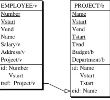
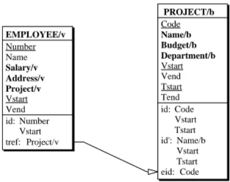
Fig. 2. A logical relational schema showing the transaction/valid timestamp columns. Tables and
columns can have time-tags. EMPLOYEE.Project is a temporal foreign key to PROJECT, whose column Name is the entity identifier (eid).
3.4 Foreign Keys
Let us first define this concept for non bitemporal tables. A column or a set of columns FK of a source table S is a foreign key to the target table T, with the primary key (PK,Start), if, for each state s of S where FK is not null, and for each time point p in [s.Start,s.End), there exists at least one state t in T such that s.FK=t.PK and t.Start≤p < t.End. This property, which must be checked when tuples are inserted, updated and deleted, is complex and expensive to evaluate for temporal databases in which the target tables are only required to be normalized or even correct [12].
In this model, a foreign key belongs to an entity or relationship table, but the target table always is an entity table. Considering that entity tables are fully normalized by construction (no gap, no overlap), the definition degenerates into a property that is more straightforward and easier (i.e., cheaper) to check. Let us consider the source table S(..., Start, End, ..., FK) and the target table T(PK, Start, End, ...). S.FK is a tempo-ral foreign key to S iff,
∀s∈S, ∃t1, t2∈T:
t1.PK= t2.PK=s.FK ∧ t1.Start≤s.Start < t1.End ∧ t2.Start < s.End≤t2.End For bitemporal databases, this definition must be valid for each snapshot.
The foreign key, its source table and its target table need not have the same time-tag. For instance, a non temporal foreign key (in a temporal or non temporal source table) can reference a non temporal (including monotonic) or a temporal table; a valid time foreign key can reference monotonic, valid time and bitemporal target table. The allowed pairs of source and target time-tags define the compatibility rules, that will not be developed further in this paper.
3.5 Operators
The semantics of the usual relational operators have been extended to temporal tables, PROJECT/b Name Vstart Vend Tstart Tend Budget/b Department/b id: Name Vstart Tstart eid: Name EMPLOYEE/v Number Vstart Vend Name Salary/v Address/v Project/v id: Number Vstart tref: Project/v
while new ones have been designed to cope with specific problems of temporal data [11]. This model includes four extraction operators, namely selection, projection, join, aggregation, and normalization transformations.
Temporal projection. This operator returns, for any correct source entity table S and for any subset A of its columns, a temporal table in which only the values of the columns in A are kept. If the set of the projection columns includes the entity identifier, the result is a normalized entity table. Conceptually, the temporal projection can be perceived as a standard projection followed by the merging (or coalescing) of the rows that have the same values of the non-temporal columns, and that either overlap or are consecutive.
Temporal selection. This operator returns the rows that meet some selection predicate
in a correct source table. The selection can involve the temporal columns, the other col-umns, or both.
Temporal join. Considering two correct temporal source tables S1 and S2, and a pred-icate P, this operator returns, for each couple of rows (s1, s2) from S1xS2 such that P is true and the temporal interval i1 of s1 and i2 of s2 overlap, a row made up of the col-umn values of both source rows and whose temporal interval is the intersection of i1 and i2. The result is a correct temporal table.
Temporal aggregation. Due to the great variety of aggregation queries, the process has
been decomposed into four steps that are easy to encapsulate. Let us consider a correct entity table T with one time dimension (the reasoning is similar for other tables). The query class coped with has the general form : select A, f(B) from T group by A, where f is any aggregation function. First, a normalized state table minT is derived by collect-ing, for each value of A, the smallest intervals during which this value appears in T10. This table is joined with T to augment it with the value s of B, giving the correct table minTval. Then, the aggregation is computed through the query select select A, f(B) from T group by A. Finally the result is coalesced. In particular, this technique pro-vides an easy way to compute temporal series (in this case, minT is a mere calendar).
Temporal normalization. This family of operators augment the consistency state (Sec.
3.2) of a correct table. By merging the value-equivalent overlapping or consecutive states, they produce normalized tables (no overlap), and by inserting the missing states of a non-fully normalized table, they produce a continuous history (no gap, no overlap).
3.6 The DML Interface
Though temporal operators can be expressed in pure SQL-92, their expression generally is complex and resource consuming [12], so that providing the programmer with a sim-ple and efficient API to manipulate temporal data is more than a necessity. Developing a complete engine that translates temporal SQL queries would have been unrealistic, so that we chose to implement a (very) small subset of a variant of TSQL2 [11], called miniTSQL, through which the complex operators, such as project, join and aggregate can be specified in a natural way and executed11. Combining explicit SQL-92 queries
10 If T(E,Start,End,A,..) has instances {(e1,20,45,a1,..), (e2,30,50,a2,..), (e3,35,55,a1,..)}, this step generates the states {(a1,20, 35), (a1,35,45), (a1,45,55), (a2,30,50)}.
11 miniTSQL and Temporal ODBC, as well as a procedural solution to bitemporal coalescing have been defined and prototyped by Olivier Ramlot (Contribution à la mise au point d’un langage d’accès aux
bases de données temporelles, Mémoire présenté en vue de l’obtention du grade de Maître en
with miniTSQL statements allows programmers to write complex scripts with reason-able effort. The API is a variant of ODBC, through which miniTSQL queries can be executed. The driver performs query analysis and interpretation based on a small repos-itory that describes the database structures and their physical implementation (Sec. 4).
The following program fragment displays the name and salary of the employees of project BIOTECH as on valid time 35. The SQL query uses a temporal projection (including coalescing) and a temporal selection. It replaces about 100 lines of complex code that would have been necessary if operating directly on the tables of Fig. 2.
char name[50], salary [20], output[100]; sdword cbname, cbsalary ;
. . .; rc=SQLConnect(hdbc,...); ...
rc=TSQLExecDirect(hdbc,hstmt,"select snapshot Name, Salary from EMPLOYEE
where valid(EMPLOYEE) contains
timepoint'35'
and Project = 'BIOTECH'",type); rc=SQLBindCol(hstmt,1,SQL_C_CHAR,name,50,cbname);
rc=SQLBindCol(hstmt,2,SQL_C_CHAR,salary,20,cbsalary); do { rc = SQLFetch(hstmt);
if(rc == SQL_NO_DATA) break;
strcpy(output,"Name: ") ; strcat(output,name); strcat(output,"Salary: "); strcat(output,salary); MessageBox(output,"TUPLE",MB_OK);
}while(rc!= SQL_NO_DATA); ...; rc=SQLDisconnect(hdbc); ...
To make the programmer’s work easier and more reliable, the modification statements insert, delete and update apply on a view that hides the transaction temporal columns Tstart and Tend. More specifically, this view returns, respectively, (1) the current states of a transaction time table, (2) all the states of a valid time table and (3) the valid history of a bitemporal table.
4
A Temporal Relational Physical Model
The physical schema describes the data structures that actually are implemented in SQL-92. When compared with the logical schema, the physical schema introduces four implementation features.
Data distribution. The logical model represents the evolution of an entity/relationship
set as a single table where each row represents a state of an entity/relationship. At the physical level, the states and the rows can be distributed, split and duplicated in order to gain better space occupation and/or improved performance. The first rule concern the distribution and duplication of states.
A bitemporal historical table includes valid current states (Tend=
∞ ∧
Vend=∞
), valid past states (Tend=∞ ∧
Vend<∞
) and invalid states (Tend<∞
). This suggest var-ious patterns of distribution, which each has advantages and drawbacks as far as perfor-mance and complexity are concerned: all the states in the same table, all the states in the same table + a copy of the valid current states in another table, the valid current states in a table + all the other states in another table, the valid states in a table + the invalid states in another table, to mention the most important. Tables with one dimension only can be organized in a similar way. Should future states be included, they would have to be stored in the same table as the current states.A logical table comprises all the columns that implement the entity attributes and the one-to-many relationship types (as foreign keys), be they temporal or not. Storing rows in a single table may induce much redundancy12, so that distributing the columns into temporally homogeneous tables can decrease it dramatically. Three patterns are of par-ticular importance: all the columns are collected in a single table (as in the logical schema), the non temporal columns form a table while a second table collects the tem-poral columns, the non temtem-poral columns form a table while each temtem-poral column forms a specific table. Other splitting patterns can be useful, that mainly pertain to the temporal normalization domain [16].
Indexing. As in conventional databases, indexes will be defined to improve the access
time for the most frequent operations. Besides the primary keys, foreign keys, argu-ments of group by and order by clauses, frequent selection criteria, are candidate for indexing. Some temporal operators can be accelerated by using auxiliary structures. For instance, an entity table that stores the life span of each entity can be used to quickly check referential constraints in a bitemporal database. A pre-join table TS, that stores, for joinable tables T and S, the couples (s,t) of rows from T and S that overlap, can be use to replace the temporal join T*S by the standard join T*TS*S, which generally is faster.
Automatic data management. Managing a physical temporal database is particular
complex, so that its automation must be pushed as far as possible. The approach we have chosen consists in implementing the logical database, as described in Sec. 3, as an
active database whose active components are responsible for guaranteeing the
consis-tency properties of the data and controlling the logical/physical mapping. Each logical table is given a set of triggers that control the insert, delete and update operations by checking their validity and by propagating them among the physical tables.
For instance, the statement,
insert into EMPLOYEE(Number,Vstart,Salary,Address,Project) values(:N,:VS,:SAL;ADD,:PRO);
triggers a procedure that performs the following operations, that can span several hun-dreds of lines of code for complex tables:
1. check: no current state where NUMBER=:N already exists (uniqueness); 2. check: no past states, where NUMBER=:N already exist (non recyclability); 3. check: Pro-ject=:PRO is a valid temporal foreign key (referential integrity); 4. check: :VS is a past or current timepoint (pure history); 5. execute: Vend is set to
∞
(current state); 6.exe-cute: the state is stored in the physical table(s) (logical/physical mapping); 7. exeexe-cute:
the auxiliary structures are updated (logical/physical mapping).
5
Methodology and CASE Support for Temporal Databases
Despite the important research area of temporal databases, few methodologies for tem-poral databases design have been developed.
Some mappings from temporally extended ER models to relational model have been proposed [5], [7], [10], [15]. The models of [5], [7], [15] support only valid time, while
12 The change of a single column in a row triggers the insertion of a new state, in which all the unchanged columns are merely copied.
the TempEER model [10] supports both valid time and transaction time of data. The TIMEER model [7] captures aspects such as the life span, valid time and transaction time of data too. A set of 31 constraints is defined to enforce the ER-specified time-related semantics in the relational context.
Those mappings allow to configure temporal data in only one way. However, we saw in Sec. 4 that it was possible to distribute data differently. Each data configuration has advantages and drawbacks, and designers must choose the distribution that corresponds best to the needs of their application. So, it would be interesting to allow different con-figurations, while hiding their complexity to the programmer.
Most often, the mappings are not supported by tools. However, the design of even modest temporal databases can prove very complex so that it cannot, most of the time, be carried out without the support of CASE tools. To mention one example only, a single
update trigger controlling a bitemporal table with two foreign keys and referenced by
another one, and that supports evolution and correction modifications, can be made up of more than 500 lines of complex code.
We will propose a solution to this problem in terms of the TimeStamp methodology for temporal databases design and of an extension of the CASE tool DB-Main that sup-ports it. The products of the methodology are the temporal conceptual, logical and phys-ical schemas, as well as the code necessary to manage and exploit the corresponding temporal relational database, as described in Sections 2, 3 and 4. The CASE tool allows to execute automatically all the processes of the methodology, including code genera-tion, according to three different physical data configurations.
In this section, we first describe the conventional methodology, then we present its extension to temporal data together with the CASE tool DB-Main.
5.1 Conventional Methodology
Database design is usually carried out in three main phases: conceptual design (or anal-ysis), logical design and physical design.
Conceptual design consists in expressing the concepts of the application domain into a high-level abstract model that is independent of the particular data model of the target DBMS. This expression is called the conceptual schema. The goal of logical design is to translate the conceptual schema into a structure adapted to the data model of the DBMS, namely the logical schema. In short, the logical schema is all the programmer have to know, and nothing more, in order to develop programs on the database. Physical design includes choosing technical implementation (e.g., indexes, data storage and clus-ters) and setting physical parameters.
These methodologies are now mastered and can be considered a integral part of the culture of developers.
5.2 Extension of the Methodology to Temporal Databases and CASE Tool DB-Main
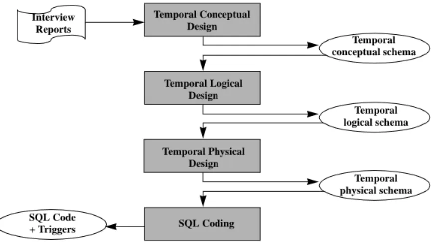
The methodology we propose is quite similar to the conventional one. Addressing the temporal dimension of data, merely adds new aspects to the standard processes (Fig. 3).
Fig. 3. Temporal Database Design Methodology. The information source is symbolically
represented by Interview reports.
The tool that is being developed in the TimeStamp project is built as a plug-in of the DB-MAIN generic CASE platform [3]. It supports all the processes of the TimeStamp methodology, including code generation. In this section, we describe the different steps of the methodology and illustrate the main aspects of the tool through the processing of an example.
5.3 Conceptual Design
Temporal conceptual design is made up of three steps: non temporal analysis, temporal tagging and normalization.
Analysis and Temporal Tagging. In this first step, a non-temporal conceptual schema
is built according to any standard methodology. Then, the schema objects that are to be temporally dimensioned are marked with the desire time-tag, namely transaction, valid, bitemporal or monotonic, as shown in Fig. 4.
Fig. 4. Example of raw (un-normalized) temporal conceptual schema. An entity primary identifier
is declared by the clause id. The tag /t, /v, /b, /m shows that the entity type, the relationship type or the attribute is timestamped with transaction time (t), valid time (v), both (b=bitemporal) or is monotonic (/m, for entity types only).
CASE support. DB-MAIN includes a graphical schema editor that allows designers to
define their schemas according to various styles (UML, ERA, OO, etc.). A special prop-erty (T_HistoryType) is attached to each data structure to define its temporal character-istics. The designer chooses the way object names are tagged to show this property graphically (Fig. 4 and Fig. 5)
Temporal conceptual schema Temporal logical schema SQL Code + Triggers Interview Reports Temporal physical schema Temporal Logical Design Temporal Physical Design SQL Coding Temporal Conceptual Design 1-1 works/b 0-N PROJECT/b Name/b Budget/b Department/b id: Name/b EMPLOYEE/v Number Name Salary/v Address/v id: Number
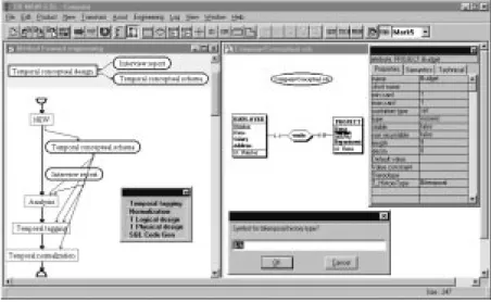
Fig. 5. .Temporal conceptual design. The main window is that of DB-MAIN. The left hand side window shows the structure of the temporal conceptual design process. The toolbar located in this window is specific to temporal database design. It allows the automatically execution of the main four processes of the methodology. The designer draws the conceptual schema in the right side windows. The right side box shows the properties of the selected object Budget. The property
T_HistoryType defines the type of time of the object (Bitemporal). The small box below permits to choose a suffix or a prefix to add automatically to the name of the temporal objects (represented by $). To tag objects, the designer selects a set of objects, then chooses the corresponding time-tag.
Normalization. Though the concept of normalized conceptual schema is well defined,
introducing the time dimension induces new criteria of normalization. In short, a tem-porally normalized conceptual schema satisfies the consistency rules defined in Sec. 2.
As an example, the schema of Fig. 4 violates rule 5: the relationship type works is
bitemporal while its 1-1 role is valid-time (this will introduce a temporal heterogeneity
in the future relational table EMPLOYEE). To fix this problem, we can either mark
works as valid time (Fig. 6).
The primary identifier of PROJECT, namely Name, is marked as temporal, violating rule 3. Therefore, we create a stable and non recyclable technical primary identifier Code, while Name becomes a secondary identifier (Fig. 6).This schema now meets all the normalization criteria.
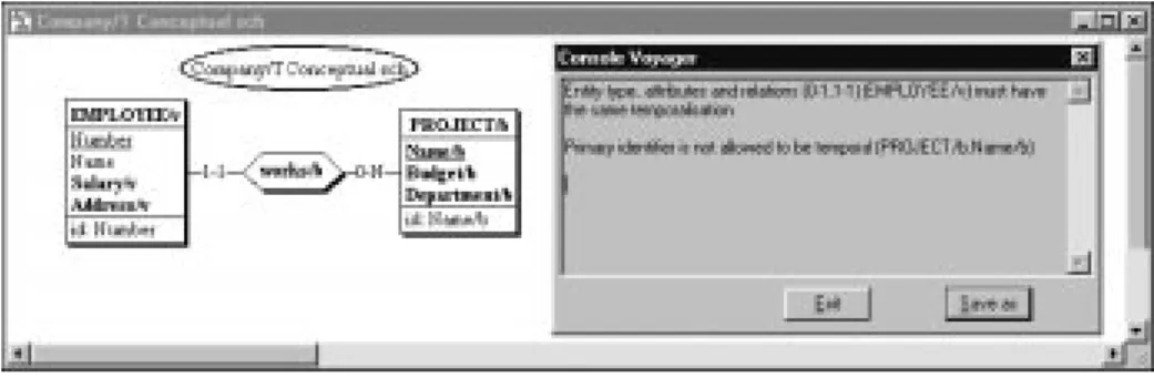
CASE Support. The tool checks the properties that a conceptual schema must satisfy.
The normalization rules that are violated are reported (Fig. 7).
Fig. 6. Normalizing temporal relationship type works (left) and making entity primary identifiers non temporal, while preserving the origin uniqueness constraint (rigth).
1-1 works/v 0-N PROJECT/b Name/b Budget/b Department/b id: Name/b EMPLOYEE/v Number Name Salary/v Address/v id: Number 1-1 works/v 0-N PROJECT/b Code Name/b Budget/b Department/b id: Code id': Name/b EMPLOYEE/v Number Name Salary/v Address/v id: Number
Fig. 7. Temporal normalization tool. The checked schema is in the window. The box on the rigth
cites the violated rules.
5.4 Logical Design
The temporal logical design phase consists in translating the conceptual constructs into relational structures and in adding the timestamp columns Vstart, Vend, Tstart and Tend as needed. Regarding the translation process, though sophisticated rules can be designed, we will adopt very simple mapping rules. According to them, an entity type is represented by a table, an attribute by a column, a many-to-many or N-ary relationship type into a table and foreign keys and a one-to-many relationship type by a mere foreign key.
The time tag of a relational construct is inherited from the conceptual object it derives from (Fig. 8). The temporal columns are then added: Vstart and Vend for the valid time and bitemporal tables, and Tstart and Tend for the transaction time and bitemporal tables. The primary keys are defined: (EI,Vstart), (EI,Tstart) and (EI,Vstart,Tstart) for respectively valid time, transaction time and bitemporal tables of entity tables. Similar rules applies for relationship tables. Where needed, the foreign keys are made temporal (Fig. 8).
As far as data management is concerned (through insert, delete, update statements), users can only manage current histories. They work then on a view that has the same configuration as the relational schema but that contains only the current histories, that is to say, all the states of a valid time table, the current states (Tend=
∞
) of a transaction time table, and the valid states (Tend=∞
) of a bitemporal table.CASE Support. The tool automatically transforms conceptual structures into relational
constructions including inherited temporal tags. It adds the timestamp columns and defines the temporal foreign keys (Fig. 8).
5.5 Physical Design
During the temporal physical design, operational and performance issues are consid-ered. Since no specialized technologies can be relied on, we have to stick to pure SQL-92 data structures. Three optimization techniques are proposed.
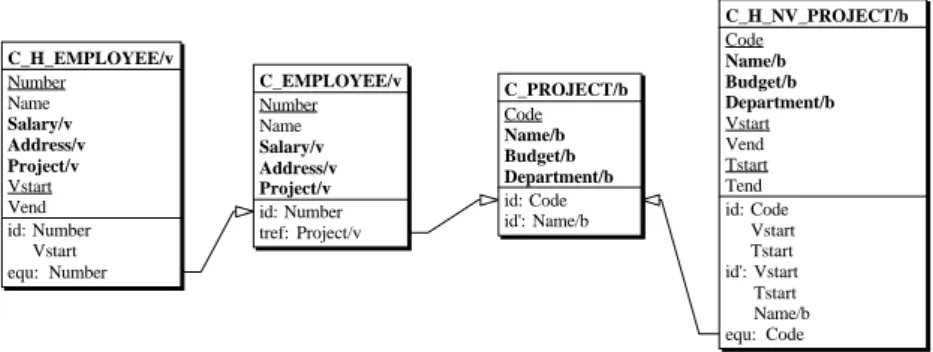
1. Table partitioning. As briefly discussed in Sec. 4, states and columns can be distrib-uted in different tables to improve the execution time of selected operations. The schema of Fig. 9 shows an example of physical schema in which the current states of
each logical table have been duplicated into the specific tables C_EMPLOYEE and C_PROJECT.
2. System index. Standard index must be defined in order to support the most common temporal and non-temporal operations. They are described for mono-temporal tables only, to simplify the discussion. A primary key index <EI,Start> supports (1) entity history and single state extraction, (2) projection and coalescing that include the entity primary identifier, (3) FK-to-PK temporal joins. An index on a temporal for-eign key <FK,Start> supports PK-to-FK joins and FK selection. Extracting the cur-rent state of an entity can be improved by a <EI,End> index, though segregating current states in a specific table will generally be more efficient. Selecting the states that fall in a time interval will profit from an index on <Start,EI>.
3. Auxiliary structures. Besides standard index, additional technical tables can be built to accelerate such operations as temporal aggregation, temporal join or projections, as discussed in Sec. 4.
CASE Support. A state data distribution strategy must be chosen. At the present time,
three predefined strategies are available, where temporal and non-temporal columns are all grouped in the same table:
1. all the states are in the same table;
2. a table contains the current states and another table the past and invalid states; 3. all the states are gouped in a same table and the current states are duplicated in a
spe-cific table (Fig. 9).
The temporal constraints known by the programmers at the logical level must be adapted for each of the three data configurations at the physical level. The expression of the con-straints at the physical level remains hidden from the programmers, and those rules will be automatically managed by the triggers of the database.
Fig. 8. Temporal logical design. The relationship types have been transformed into foreign keys and the temporal columns have been added. The clause tref symbolizes a temporal foreign key (temporal reference). The arc indicates the target candidate key, which is the entity identifier (eid).
SQL Code Generation. Managing and exploiting temporal data involves a high
pro-gramming overhead. Therefore, it is important to relieve programmers from the burden of writing this code him/herself. The design of the database must include the writing all the technical procedures, particularly the triggers, that manage the tables and keep them in a consistent state. PROJECT/b Code Name/b Budget/b Department/b Vstart Vend Tstart Tend id: Code Vstart Tstart id': Name/b Vstart Tstart eid: Code EMPLOYEE/v Number Name Salary/v Address/v Project/v Vstart Vend id: Number Vstart tref: Project/v
CASE Support. A tool generates automatically the SQL code that implements the
physi-cal schema. This code can be processed by Oracle 8 and includes the definitions of the tables, views, indexes and triggers necessary to manage the temporal data, according to the physical parameters chosen by the developer. The generation of the temporal ODBC drivers, that implement the stratum architecture, still is under development.
Fig. 9. Physical schema. The clause equ symbolizes an equality constraint, that combines a
foreign key (ref) with an inverse inclusion constraint. For each logical table, a complete history table is maintained, together with a new table that includes the current states.
6
Conclusion
The goal of the TimeStamp project, which started in 1997, was to make, as much as pos-sible, the research results in temporal databases available to practitioners, i.e., standard developers and programmers. Considering the richness and the complexity of the con-cepts of this domain, most of our effort was devoted to simplify them, while retaining enough power and flexibility for making them usable in practical situations.
The simplification has addressed two directions. First, the concepts have been reduced in order to make them easy to understand and to teach. The simplified temporal conceptual model induces a reduced temporal relational logical model, which in turn implies simple and efficient data management techniques. In addition, the methodology we propose is a slight extension of widespread approaches. Secondly, all the burden of developing temporal databases has been taken in charge by a CASE tool and an API has been defined and implemented to make the programming process easier and, more important, more reliable.
Despite this effort, mastering temporal database concepts still is a challenging task, as we experienced when teaching them to practitioners. In particular, understanding bitemporal databases and their dynamic behavior has proved very difficult, and often out of the competence of many ordinary programmers. Since the problem lies in the inter-pretation of bitemporal data, it cannot be completely solved by merely automating the development processes. Therefore, we consider that education is a major aspect of dif-fusing temporal database principles, at least as important as developing automated tools and API.
Several questions and points remain unsolved: optimized physical design in the con-text of the stratum architecture, migration of legacy data to temporal database and cop-ing with schema evolution [4].
C_PROJECT/b Code Name/b Budget/b Department/b id: Code id': Name/b C_H_NV_PROJECT/b Code Name/b Budget/b Department/b Vstart Vend Tstart Tend id: Code Vstart Tstart id': Vstart Tstart Name/b equ: Code C_EMPLOYEE/v Number Name Salary/v Address/v Project/v id: Number tref: Project/v C_H_EMPLOYEE/v Number Name Salary/v Address/v Project/v Vstart Vend id: Number Vstart equ: Number
7
Credits
Jeff Wijsen kindly reviewed our results and made several important suggestions to improve the models. Babis Theodoulidis and his staff, hosted O. Ramlot during his stay in UMIST, Manchester. Their comments were essential for the definition of the temporal ODBC interface. Ramez Elmasri, who hosted one of our students too, helped him to understand and master physical implementation of temporal databases. Thanks to them.
References
1.BÖHLEN M., Temporal Database System Implementations, ACM SIGMOD Record, 24(4):53-60, December, 1995.
2.BÖHLEN M., Coalescing in Temporal Databases, Proc. of the 22nd VLDB Conference, Bom-bay, India, 1996.
3.DB-MAIN, http://www.db-main.be
4.ELMASRI R., WEI H., Study and Comparison of Schema Versioning and Database Conversion
Techniques for Bi-temporal Databases, Proceedings of the Sixth International Workshop on
Temporal Representation and Reasoning (TIME-99), Orlando, Florida, May 1999, IEEE Com-puter Society.
5.FERG S., Modeling the Time Dimension in an Entity-Relationship Diagram, Proceedings of the 4th International Confernce on the Entity-Relationship Approach, pages 280-286, Siver Spring, MD, 1985.
6.GREGERSEN H., JENSEN C. S., MARK L., Evaluating Temporally Extended ER Models, Pro-ceedings of the Second CAISE/IFIP8.1 International Workshop on Evaluation of Modeling Methods in System Analysis and Design, 12p, K. Siau, Y. Wand, J. Parsons, editors, Barce-lona, Spain, June 1997.
7.GREGERSEN H., MARK L., JENSEN C. S., Mapping Temporal ER Diagrams to Relational
Schemas, Technical Report TR-39, Aalborg University, Department of Mathematics and
Com-puter Science, December 1998.
8.HAINAUT, J.-L., ROLAND, D., HICK, J.-M., HENRARD, J., ENGLEBERT, V., Database Reverse Engineering: from Requirements to CARE tools, Journal of Automated Software
Engineering, Vol. 3, No. 2, 1996
9.JENSEN C., SNODGRASS R., Temporal Data Management, Technical Report TR-17, TIMECENTER, 1997.
10.LAI V.S., KUILBOER J-P., GUYNES J. L., Temporal Databases : Model Design and
Com-mercialization Prospects, DATA BASE, 25(3), 1994.
11.SNODGRASS R., The TSQL2 Temporal Query Language, Kluwer Academic Publishers, Mas-sachussetts, USA, 1995.
12.SNODGRASS R., Developing Time-Oriented Database Applications in SQL, Morgan Kauf-mann Publishers, USA, 2000.
13.STEINER A., A Generalisation approach to Temporal Data Models and their
Implementa-tions, Thesis of the Swiss Federal Institute of Technology for the degree of Doctor of
Techni-cal Sciences, Zürich, 1998.
14.SVINTERIKOU M., THEODOULIDIS C., The Temporal Unified Modelling Language, Department of Computation, UMIST, United Kingdom, October 1997.
15.THEODOULIDIS C.I., LOUCOPOULOS P., WANGLER B., A Conceptual Modelling
Forma-lism for Temporal Database Applications, Information Systems, 16(4), 1991.
16.WIJSEN J., Temporal FDs on Complex objects, ACM Transactions on Database Systems, Vol 24., No.1,Pages 127-176, March 1999