Improving tropical forest aboveground biomass estimations: insights from canopy trees structure and spatial organization

HAL Id: tel-01624428

https://tel.archives-ouvertes.fr/tel-01624428

HAL is a multi-disciplinary open access

archive for the deposit and dissemination of sci-entific research documents, whether they are

pub-L’archive ouverte pluridisciplinaire HAL, est destinée au dépôt et à la diffusion de documents scientifiques de niveau recherche, publiés ou non,

Improving tropical forest aboveground biomass

estimations: insights from canopy trees structure and

spatial organization

Pierre Ploton

To cite this version:

Pierre Ploton. Improving tropical forest aboveground biomass estimations: insights from canopy trees structure and spatial organization . Biodiversity and Ecology. AgroParisTech, 2017. English. �tel-01624428�

AgroParisTech - IRD

N°: 2017AGPT0005

présentée et soutenue publiquement par

Pierre PLOTON

Improving tropical forest aboveground biomass estimations:

insights from canopy trees structure and spatial organization

Doctorat AgroParisTech

T H È S E

pour obtenir le grade de docteur délivré par

L’Institut des Sciences et Industries

du Vivant et de l’Environnement

(AgroParisTech)

Spécialité : Ecologie et Biodiversité

Directeur de thèse : Dr. Raphaël PELISSIER Co-encadrement de la thèse : Prof. Dr. Uta BERGER

Jury

M. Lilian BLANC, Chercheur (HDR), CIRAD Rapporteur

M. Laurent SAINT-ANDRE, Directeur de Recherche, INRA Rapporteur

M. Hans-Gerd MAAS, Professeur, Technische Universität Dresden Rapporteur

M. Pierre COUTERON, Directeur de Recherche, IRD Président

Mme Uta BERGER, Professeur, Technische Universität Dresden Co-directeur de thèse

A

CKNOWLEDGEMENTS

This doctoral thesis was realized thanks to the support of the 2013-2016 Forest, Nature and Society (FONASO) grant, funded by the European Commission’s Erasmus Mundus Joint Doctorate programme (EMJD). Part of the thesis was funded by the CoForTips project as part of the ERA-Net BiodivERsA 2011-2012 European joint call (ANR-12-EBID-0002). I am also grateful for the multiple travelling funds I received from the UMR AMAP of the French Institut de Recherche pour le Développement (IRD).

I have benefited from the support, advices and help of numerous people during the 3 (and a half…) years of this PhD project. First and foremost, I would like to thank Dr. Raphaël Pélissier, who’s been supervising my work since my first steps in the world of forest research, about 7 years ago at the French Institute of Pondicherry. I’m deeply indebted to you for the opportunity you gave me to work on such fascinating subjects during the past years. For your incredible patience while reading long and sometimes crazy “results syntheses” I’ve been sending you, for helping me to see broader implications rather than details in my analyses, for your positive attitude toward our findings, thank you. I am also very grateful to Prof. Uta Berger, who kindly provided support and guidance during this project, and made this Joint Doctoral Programme a very positive experience for me.

I must also warmly thank Dr. Nicolas Barbier for the considerable amount of time we spent, at the office or in the field, brainstorming about our common research interests. Beyond invaluable scientific guidance, total availability for my questions and concerns, deep involvement in the different projects we undertook, you’ve simply been of great company, and I’m thankful for the tons of fun we had in the field.

This list is far from being exhaustive, but I should also mention my deep gratitude to Dr. Pierre Couteron, Dr. Christophe Proisy and Dr. Maxime Réjou-Méchain for the fruitful discussions we had, notably on FOTO texture and biomass allometric models. I am also very grateful to Dr. Gilles Le Moguedec for his availability and good will to help me resolve statistical issues I’ve been having throughout this project.

Last but not least, this PhD project largely beneficiated from the field work several colleagues and I carried out in Cameroon. I owe a great deal of thanks to Prof. Bonaventure Sonké, who warmly welcomed me in his research team and created a pleasant and efficient working environment. I’d also like to thank Dr. Vincent Droissart with whom, just like with Nicolas, I spent a formidable time in the field. My thoughts also go to the Cameroonian students and friends I’ve been collecting field data with, notably S.T. Momo, M. Libalah, N.G. Kamdem, H. Taedoumg, G. Kamdem Meikeu and D. Zebaze.

T

ABLE OF CONTENTS

1 GENERAL INTRODUCTION...1

1.1 Context and challenges ...1

1.1.1 Tropical forests and climate change ...1

1.1.2 REDD monitoring frame of tropical forest biomass: basics and challenges ...2

1.1.3 Remote sensing-based modelling of tropical forest biomass ...4

1.2 Research objectives...8

1.3 A pantropical approach ...9

1.3.1 Study areas and datasets ...9

1.3.2 Sampling strategy and data description ... 11

1.4 Thesis outline ... 12

1.5 List of (co-)publications ... 13

1.6 References ... 14

2 CLOSING A GAP IN TROPICAL FOREST BIOMASS ESTIMATION:ACCOUNTING FOR CROWN MASS VARIATION IN PANTROPICAL ALLOMETRIES ... 19

2.1 Introduction ... 20

2.2 Materials and Methods ... 22

2.2.1 Biomass data ... 22

2.2.2 Forest inventory data ... 22

2.2.3 Allometric model fitting ... 22

2.2.4 Development of crown mass proxies... 23

2.2.5 Model error evaluation ... 24

2.3 Results ... 25

2.3.1 Contribution of crown to tree mass... 25

2.3.2 Crown mass sub-models ... 25

2.3.3 Accounting for crown mass in biomass allometric models ... 28

2.4 Discussion ... 32

2.4.1 Crown mass ratio and the reference biomass model error ... 32

2.4.2 Model error propagation depends on targeted plot structure ... 33

2.4.3 Accounting for crown mass variation in allometric models ... 33

2.5 Appendix A: Crown mass sub-models ... 34

2.5.1 Method... 34

2.5.2 Results & Discussion ... 34

2.6 Appendix B: Plot-level error propagation ... 38

2.7 References ... 41

2.8.1 Unpublished dataset: site characteristics ... 46

2.8.2 Biomass data ... 46

2.8.3 Inventory data ... 48

3 ASSESSING DA VINCI’S RULE ON LARGE TROPICAL TREE CROWNS OF CONTRASTED ARCHITECTURES: EVIDENCE FOR AREA-INCREASING BRANCHING ... 49

3.1 Introduction ... 49

3.2 Methods ... 51

3.2.1 Sampled trees and field protocol ... 51

3.2.2 MTE model assumptions and predictions of branch scaling exponents ... 53

3.2.3 Assessing the effect of asymmetry and node morphology on species area ratio ... 54

3.3 Results ... 55

3.3.1 Does the average tree conform to branch scaling exponents and area ratio predictions? ... 55

3.3.2 Is the average tree self-similar?... 55

3.3.3 What is the effect of species asymmetry on branch scaling exponents and area ratio? . ... 56

3.3.4 Does node morphology induce systematic differences of area ratio at the species level? ... 58

3.4 Discussion ... 59

3.4.1 Evidence of area increasing branching (R > 1) ... 59

3.4.2 Sources of variation of the node area ratio ... 60

3.4.3 Optimal tree of the MTE model vs average real trees ... 62

3.4.4 Implications of the results ... 64

3.5. Reference... 65

3.6. Supplementary figure ... 68

4 CANOPY TEXTURE ANALYSIS FOR LARGE-SCALE ASSESSMENTS OF TROPICAL FOREST STAND STRUCTURE AND BIOMASS ... 69

4.1 Introduction ... 70

4.2 Methodological background and rationale ... 70

4.3 Results from some case studies ... 72

4.4 Limits and perspectives ... 75

4.5 Reference ... 76

5 TOWARD A GENERAL TROPICAL FOREST BIOMASS PREDICTION MODEL FROM VERY HIGH RESOLUTION OPTICAL SATELLITE IMAGES ... 77

Abstract ... 77

5.2.3 Simulation of canopy images... 82

5.2.4 Real satellite images ... 82

5.2.5 Canopy texture analysis ... 83

5.2.6 Statistical analyses ... 84

5.3 Results ... 85

5.3.1 Texture analysis of virtual canopy images ... 85

5.3.2 Canopy texture - AGB models ... 89

5.3.3 Application to real satellite images... 91

5.4 Discussion ... 91

5.4.1 Contrasted canopy texture - stand AGB relationships among sites ... 92

5.4.2 On 3D stand mockups and virtual canopy images for model calibration ... 93

5.5 Reference ... 95

5.6 Appendix ... 100

6 GENERAL DISCUSSION ... 102

6.1 Estimation of forest AGB from field data ... 102

6.1.1 Driver(s) of pantropical model bias on large trees ... 102

6.1.2 The influence of forest structure on plot-level AGB modelling error ... 105

6.2 The influence of forest structure on the canopy texture – AGB relationship ... 106

6.3 Key thesis findings ... 110

L

IST OF FIGURES

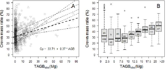
Figure 1-1. General workflow of remote sensing-based AGB mapping methods. Regardless of the remote sensing data type, remote sensing indice(s) are extracted over forest sample plots (A) and used a predictor(s) of in situ AGB estimations (B). Once calibrated, the model can be used to predict forest AGB over the entire study area (C). ...4 Figure 1-2. Schematic illustration of virtual canopy scenes simulation procedure. Field inventory data are used in a forest model to generate 3D mockups of the sample plots. A radiative transfer model simulates a satellite view of the mockups, for instance a VHSR 1-m IKONOS panchromatic channel. ...6 Figure 1-3. Distribution of datasets across the tropics. Dots and triangles represent tree-level destructive datasets and field plot inventories, respectively. Red color indicates that data have been collected by IRD. Blue color indicates that data were compiled from literature, collaborating institutions or shared by the peer researchers. ... 10 Figure 1-4. VHSR satellite image (GeoEye sensor) covering a typical forest mosaic from semi-deciduous forests of south-eastern Cameroon. Patches of Gilbertiodendron dewevrei (black square), mixed closed-canopy stands (red square) and open-canopy Marantaceae stands closely co-occur. ... 11 Figure 2-1. (A) Distribution of crown mass ratio (in %) along the range of tree mass (TAGBobs, in Mg) for

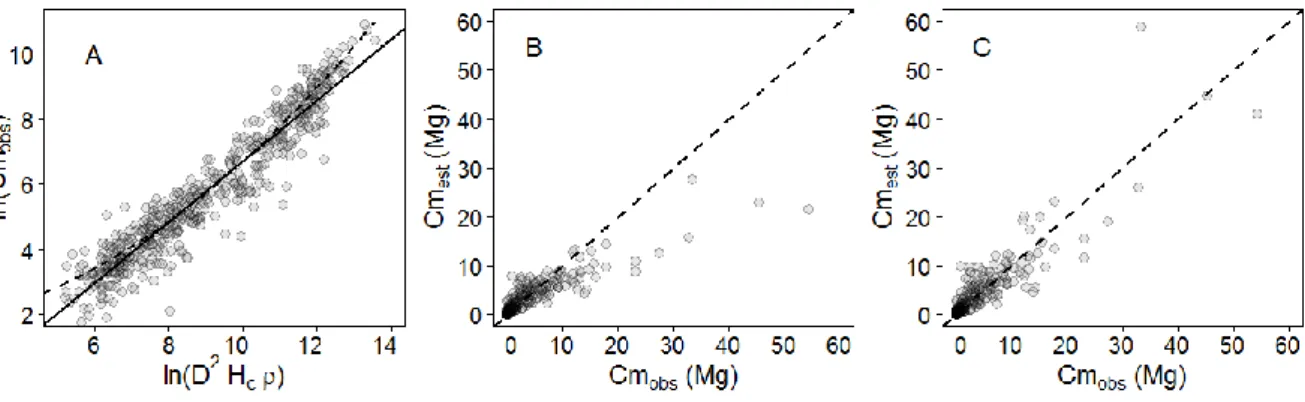
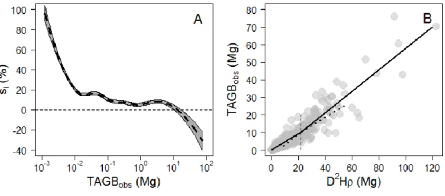
673 trees. Dashed lines represent the fit of robust regressions (model II linear regression fitted using ordinary least square) performed on the full crown mass dataset (thick line; one-tailed permutation test on slope: p-value < 0.001) and on each separate source (thin lines), with symbols indicating the source: empty circles from Vieilledent et.al. (2011; regression line not represented since the largest tree is 3.7 Mg only); solid circles from Fayolle et.al. (2013); squares from Goodman et al. (2013, 2014); diamonds from Henry et.al. (2010); head-up triangles from Ngomanda et.al. (2014); and head-down triangles from the un-published data set from Cameroon. (B) Boxplot representing the variation in crown mass ratio (in %) across tree mass bins of equal width (2.5 Mg). The last bin contains all trees ≥ 20 Mg. The number of individuals per bin and the results of non-parametric pairwise comparisons are represented below and above the median lines, respectively. ... 26 Figure 2-2. (A) Observed crown mass versus the compound variable D²Hcρ (in log scale), displaying a slightly concave relationship. The crown mass sub-model 1 does not capture this effect (model fit represented with a full line in caption A), resulting in biased model predictions (caption B), whereas sub-model 3 does not present this error pattern (model fit represented as a dashed line in caption A, observed crown mass against model predictions in caption C). Models were fitted on DataCM2. ... 28 Figure 2-3. (A) Relative individual residuals (si in %) of the reference pantropical model of Chave et.al. (2014) against the tree AGB gradient. The thick dashed line represents the fit of a local regression (loess function, span = 0.5) bounded by standard errors. (B) Observed tree AGB (TAGBobs) versus the compound variable 𝐷2 ∗ 𝐻 ∗ 𝜌 with D and H being the tree stem diameter and height, respectively, and ρ the wood density. A segmented regression revealed a significant break point (thin vertical dashed line) at approximately 10 Mg of TAGBobs (Davies test p-value < 2.2e-16). ... 29 Figure 2-4. (A) Relative residuals (si, in %) of the reference pantropical model m0 (grey background) and

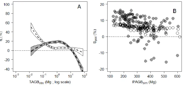
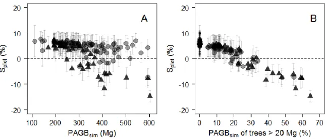
Figure 2-5. (A) Relative individual residuals (si, in %) obtained with the reference pantropical model m0 (grey background) and with our model including a crown mass proxy, m2 (white background). Thick dashed lines represent fits of local regressions (loess function, span = 1) bounded by standard errors. (B) Propagation of individual residual errors of m0 (solid grey circles) and m2 (empty circles) to the plot level. ... 30 Figure 2-6. Observed against estimated crown mass (in Mg) for models 1-D (caption A), 1-Hc (caption B), 2-D (caption C), 3 (caption D). Models were calibrated on DataCM2. Tree wood density was standardized to range between 0 and 1 and represented as a grayscale (with black the lowest values and white the highest values). ... 35 Figure 2-7. Observed versus estimated crown mass (in Mg) for models 1-D (caption A), 1-Cd (caption B), 2-D (caption C), 2-Cd (caption D). Models were calibrated on DataCD. Tree wood density was standardized to range between 0 and 1 and is represented as a grayscale (with black the lowest values and white the highest values). ... 37 Figure 2-8. Plot-level propagation of individual-level model error. (A) Mean relative error (Splot, in %) and standard deviation of 1000 random error sampling against simulated plot AGB and (B) against the fraction (%) of simulated plot AGB accounted for by trees > 20 Mg. Plots from Korup permanent plot are represented by triangles. ... 39 Figure 2-9. Plot-level relative error (Splot, in %) as a function of plot size (in ha) in Korup permanent plot. Individual plot values are represented by grey dots. ... 39 Figure 3-1. Schematic representation of different levels of asymmetry in species’ architecture, from the optimal MTE tree (A) to moderately (B) and highly (C) dominant apex. O1 to O4 represent the labeling scheme of the MTE. In panel C, Om1 to Om2 illustrate a modified labeling scheme accounting for the presence of a principal axis in tree crown structure (see text). The right column gives illustrations of the three types of architectures based on large canopy tree species from central Africa, from top to bottom: Okan, Ayous and Ilomba (see Table 3-1 for more information on these species). ... 52 Figure 3-2. Distribution of sampled nodes along node parent diameters (in cm) in each of the 9 sampled species. ... 52 Figure 3-3. Frequency of PA internodes per species. Ilomba (35.7% : highly asymmetric), Ayous (9.4% : moderately asymmetric) and Okan (1.3%: symmetric) were selected as illustrative species in results sections 3.3 and 3.4. ... 54 Figure 3-4. Density distributions (standardized to 1) of internodes length scaling exponents (A), radii scaling exponents (B) and nodes area ratios (C) at the inter-specific level. Dash lines represent the expected values under the Metabolic Theory of Ecology, while grey bars represent the 95% confidence interval of resampled medians (A, B) and mean (C). ... 55 Figure 3-5. Density distributions (standardized to 1) of internodes length scaling exponents (A), radii scaling exponents (B) and nodes area ratios (C) across the first orders (i.e. 2, 3, ≥ 4) of the centrifugal labeling scheme. We excluded internodes of parent order 1 (i.e., the trunk) from analysis of length scaling exponents (in panel A). Dash black lines represent the expected values for hierarchical, symmetric, self-similar trees. Color bars represent the 2.5-97.5% interval of resampled medians per group. Branch scaling exponents and area ratios are also represented against parent diameter (D, E, F). ... 56 Figure 3-6. Density distributions (standardized to 1) of internode length scaling exponents (A, B), internodes radii scaling exponents (C, D) and node area ratios (E,F). In plots A, C and E, parameters are

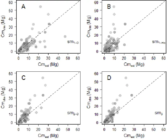
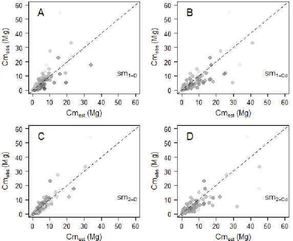
given for 3 illustrative species (i.e., Ayous, Ilomba and Okan) with contrasted frequency of PA internodes (cf. fig 3). Distributions are based on all internodes and nodes from those species, regardless of node morphology. In plots B, D and F, distributions are based on all data (inter-specific) split by node morphology i.e., internodes and nodes were grouped according to the presence of a PA, thus differentiating PA branches, their sibling(s) and branches from nodes w/o PA branch (noted “Other”). Dash black lines represent the expected values for hierarchical, symmetric, self-similar trees. Color bars represent the 2.5-97.5% interval of resampled medians per group. ... 57 Figure 3-7. (A) Density distribution of nodes area ratio for nodes with 2 (light grey) and >2 daughters (dark grey). (B) Nodes area ratio against daughters asymmetry (‘q’). Thick and thin dashed lines represent fits of linear models on nodes bearing (dark grey) or not bearing (light grey) PA branches, respectively. (C, D) Daughters cumulated area against parent area (in true unit). The upper limits of plots axes was set to 1.5 m² to ease species comparison, as branch cross-sectional areas for the Ayous species extend above c. 2.5 m². Dashed lines represent the fits of linear models on both Ayous and Ilomba (black line) and Okan (grey line). Linear models were adjusted on log-transformed data. ... 59 Figure 3-8. Histograms of log-transformed abundance against log-transform branch diameter (panel A) and branch length (panel B) for all nine species. Daughters dimensions (diameter, length) against parents dimensions (diameter length) are represented in panel C and D, with a color code differentiating PA daughters (solid black circles) from other daughters (solid grey circles). In panel E and F, the number of daughters (nD) is represented against parent order and per illustrative species, respectively. In panel E, the labelling scheme used to defined parent order is either the centrifugal scheme of the MTE (solid black circles) or the modified labelling scheme distinguishing PA daughters (order 1), their siblings (order 2) and other daughters (order ≥ 3) (empty circles). In panel F, a distinction is made between nodes bearing PA daughters (solid black circles) and others nodes (empty circles). Letters represent the result of Dunn pairwise multiple comparisons tests... 68 Figure 4-1. Flow of operations of the FOurier Textural Ordination (FOTO) method. ... 72 Figure 5-1. Canopy texture ordinations based on (A) the FOTO method and (B) the lacunarity analysis. In both cases, scatter plots of PCA scores along the first two principal axes are shown, with 3 example sites highlighted with particular symbols (Paracou, Uppangala and Yellapur). Correlation circles are given with wavelength, λ (A) or box size, s (B) in meter. Histograms of eigenvalues in % of total variance. ... 86 Figure 5-2. Co-inertia analysis. Position on the first co-inertia plane of the FOTO r-spectra wavelengths, λ (A) and the lacunarity box size, s (D). Components of the F-PCA (B) and the L-PCA (E) projected onto the co-inertia axes. Ordination of windows from the 3 example sites (Paracou, Uppangala and Yellapur) on COIA-1 (C) with large empty and full circles representing the average site-level score for FOTO and Lacunarity features, respectively. Normed scores of 10 randomly sampled canopy windows from the 3 example sites on the first co-inertia plane (F), with each arrow linking a canopy window position for FOTO and Lacunarity characteristics, respectively. ... 89 Figure 5-3. Multi-site AGB prediction models based on FOTO texture (F-model), Lacunarity texture

(L-model), the two sources of texture information (FL-model) to which we also added a forest canopy height proxy E (FLE-model). Texture features were extracted from virtual canopy scenes. Goodness of

Figure 5-4. Multi-site AGB prediction model over 49 1-ha plots in central Africa, based on both FOTO-texture and Lacunarity-FOTO-texture indices to which we added the bioclimatic stress variable E as a proxy of potential canopy height (FLE-model). ... 91 Figure 6-1. Field-derived AGB vs AGB predicted from the pantropical model of Chave et. al (2014). Circles represent the trees of Chave et al. (2014) destructive database, with the red color highlighting the trees sampled in the frame of this thesis. Stars represent Entandrophragma excelsum individuals sampled by Hemp et al. (2016)... 105

Figure 6-2. Tree density (N) against quadratic mean diameter (Dg) at two sites (black: Paracou, blue: Deng-Deng). Grey dot lines represent basal area (G) isolines. ... 108

L

IST OF TABLES

Table 2-1. Crown mas sub-models. Model variables are Cm (crown mass, Mg), D (diameter at breast height, cm), Hc (crown depth, m), Cs (average of Hc and crown diameter, m) and ρ (wood density, g.cm-3). The general form of the models is ln(Y) ~a+ b* ln(X) + c*ln(X)². Model coefficient estimates are provided along with the associated standard error denoted SEi, with i as the coefficient. Coefficients’ probability value (pv) is not reported when pv ≤ 10-4 and otherwise coded as follows: pv ≤ 10-3 : '**', pv ≤ 10-2 : '*', pv ≤ 0.05 : '.' and pv ≥ 0.05 : 'ns'. Models’ performance parameters are R² (adjusted R square), RSE (residual standard error), S (median of unsigned relative individual errors, in %), AIC (Akaike Information Criterion), dF (degree of freedom). ... 27 Table 2-2. Models used to estimate tree AGB. Model parameters are D (diameter at breast height, cm), H (total height, m), Ht (trunk height, m), Hc (crown depth, m), Cm (crown mass, Mg), Cs (average of Hc and crown diameter, m) and ρ (wood density, g.cm-3_{). The general form of the models is ln(Y)} ~a+ b* ln(X1) + c*ln(X2). Model coefficient estimates are provided along with the associated standard error denoted SEi, with i as the coefficient. Coefficients’ probability value (pv) is not reported when pv ≤ 10-4 _{and otherwise coded as follows: pv ≤ 10}-3 _{: '**', pv ≤ 10}-2 _{: '*', pv ≤ 0.05 : '.'} and pv ≥ 0.05 : 'ns'. Models’ performance parameters are R² (adjusted R square), RSE (residual standard error), S (median of unsigned relative individual errors, in %), AIC (Akaike Information Criterion), dF (degree of freedom). ... 31 Table 2-3. Sub-models used to estimate crown AGB. Model parameters are D (diameter at breast height, cm), Hc (crown depth, m), Cm (crown mass, Mg), Cd (crown diameter, in m), Cs (average of Hc and Cd, m) and ρ (wood density, g.cm-3_{). The general form of the models is ln(Y) ~ a + b*ln(X) +} c*ln(Y). Model coefficients’ estimates are provided along with the associated standard error denoted SEi, with i as the coefficient. Coefficients’ probability value (pv) is not reported when pv ≤ 10-4 _{and otherwise coded as follows: pv ≤ 10}-3 _{: '**', pv ≤ 10}-2 _{: '*', pv ≤ 0.05 : '.' and pv ≥ 0.05 : 'ns'.} Models’ performance parameters are R² (adjusted R square), RSE (residual standard error), S (median of unsigned relative individual errors, in %), AIC (Akaike Information Criterion), dF (degree of freedom)... 36 Table 2-4. Six destructive datasets providing information on tree crown were combined into three working datasets with increasing level of information. DataCM1 possess information on crown mass. DataCM2 add information on trunk height. DataCD add information on crown diameter. ... 47 Table 3-1. Number of trees sampled (ntree) among species, ranges of diameter at breast height (DBH, in cm) and apical dominance (from A low dominance to C highly dominant; see Figure 3-1 for illustration). ... 51 Table 4-1. FOTO explanatory power on several common forest stand attributes over a variety of tropical forest types. Quality of the relationships is characterized by the coefficient of determination (R²), the associated P-value (ns: > 0.05) and the relative root mean square error Rrmse (in %). Forest attributes: N = density of trees more than 10 cm dbh (trees.ha-1), N30 = density of trees more than 30 cm dbh (trees.ha-1_{), N}

-Table 5-1. Date and acquisition parameters of Pleiades panchromatic satellite images over Eastern Cameroun, central Africa ... 83 Table 5-2. Correlation between stand structure parameters extracted from three-dimensional mockups and canopy window scores on the texture ordination axes based on the FOTO method (F-PCA1 and F-PCA2) and the lacunarity analysis (L-(F-PCA1 and L-PCA2). Probability value of Pearson correlation test are provided between brackets and coded following standard notation (*** P ≤ 0.01, ** P ≤ 0.01, * P ≤ 0.05, ns = non-significant). ... 88 Table 5-3. Distribution of forest inventory data among sampling sites. Tree dimensions collected in field plots include the diameter at breast height (D), tree height (H), trunk height (Ht) and crown diameter (Cd). ... 100 Table 5-4. Importance of predictors (ie. IncMSE, in %) in RF regression models calibrated on simulated canopy scenes. Model m1 is based on FOTO-texture, m2 on Lacunarity-texture, m3 on FOTO- and Lacunarity-texture, m4 all textural indices and the bioclimatic variable E. F-PCA1 and F-PCA2 represent the 2 FOTO-texture indices. L-PCA1 and L-PCA2 represent the 2 Lacunarity-texture indices. ... 101

Table 5-5. Importance of predictors (ie. IncMSE, in %) in RF regression models calibrated on real satellite images. Model m1 is based on FOTO-texture, m2 on Lacunarity-texture, m3 on FOTO- and Lacunarity-texture, m4 all textural indices and the bioclimatic variable E. F-PCA1 and F-PCA2 represent the 2 FOTO-texture indices. L-PCA1 and L-PCA2 represent the 2 Lacunarity-texture indices. ... 101

1 G

ENERAL INTRODUCTION

This chapter provides an overview of the general research topics addressed in the course of my doctoral study. Specifically, I give a concise justification of the impetus for scientific research on tropical forest carbon and stress the crucial role of remote-sensing in this dynamic. The focus is then put on two important aspects of the remote sensing-based carbon mapping chain that I present in separate sections: (1) the actual remote sensing of forest carbon and (2) field estimations of forest carbon, which constitute the ‘ground truth’ of the mapping chain. Each section leads to broad methodological orientations that have been taken in this thesis and identifies key problems. In the end, I present the research objectives, the pantropical scope of this work and the organization of the thesis chapters.

1.1 Context and challenges

1.1.1 Tropical forests and climate change

International concerns about climate change have fostered research on the global carbon cycle, as carbon dioxide (CO2) is the largest contributor to anthropogenically enhanced greenhouse effect (Houghton, 2007). Together with the soil, terrestrial vegetation composes the “terrestrial ecosystems carbon reservoir” (Houghton et al., 2009) and interacts with the carbon cycle by fixing atmospheric CO2 (photosynthesis) and sequestrating it in plant’s material. Plants carbon is quantified through biomass (as dry weight is c. 50 % carbon), often distinguishing live biomass (above and below ground) from dead material. Among terrestrial biomes, the focus is usually put on forest ecosystems which store the vast majority of biomass stocks (c. 70-90 %) (Houghton et al., 2009), and within forest biomes, tropical forests are the largest ones in surface with about c. 1949 Mha (i.e. c. 50 % of total forested lands) and store approximately c. 55 % of the global forest carbon, against c. 32 % in boreal and c. 14 % in temperate forests (Pan et al., 2011). Perhaps more important to the global carbon cycle than forest carbon stocks themselves is how these stocks change in time. Forests are dynamical ecosystems presenting continuous change in forest age structure and community composition. A broadly accepted pattern of forest biomass dynamics in undisturbed systems is a fast increase early in forest succession (‘forest aggradation’ phase) followed by a gradual decrease of biomass growth rate with forest age (e.g. Ryan et al., 1997). Associated changes in stand structure properties, such as tree dimensions and spatial organization, can partly be observed from above the forest, for instance from a satellite sensor, and can be used to monitor forest biomass (as we will see in section 1.1.3.2). Growing (or re-growing) forests thus behave as carbon sinks, trapping atmospheric CO2 at different rates. On the other hand, forest carbon can be released back into the atmosphere through combustion and decomposition of forest biomass. Change in land use (i.e. deforestation) and forest degradation (e.g. logging) are the principal drivers of forest-related carbon emissions, transforming forested lands from carbon sinks into carbon sources. The tropical forest biome is the most threatened by deforestation and degradations (e.g. Pan et al., 2011). Over the 1990 - 2007 period, Pan and colleagues (2011) estimated that gross carbon emissions from tropical deforestation represented as much as c. 40 % of carbon emissions from fossil fuel combustion. This massive carbon release was however largely offset by a massive carbon uptake in this biome (representing c. 70 % of world’s forests sink), yielding a net carbon emission commonly reported around c. 12 % of total anthropogenic emissions for the first decade of the century

2007) and in turn global climate change. Based on this observation, the REDD (“Reducing Emissions from Deforestation and forest Degradation”) program was launched in Bali under the United Nations Framework Convention on Climate Change (UNFCCC, 2007), with at its core the idea that developed countries would compensate developing countries for avoided forest carbon emissions. Payments would, however, be conditional to a verified monitoring of avoided carbon emissions. Beside sociopolitical challenges that REDD poses, it also constitutes a formidable scientific challenge, as its success partly lies on our ability to accurately monitor forest carbon variation in space and time.

1.1.2 REDD monitoring frame of tropical forest biomass: basics and challenges

Estimating forests area at one point in time and its dynamics during a time period (i.e. forest area change, driven by deforestation or forest regrowth) can be achieved with remote-sensing (RS) or census data (i.e. from national forest inventories or global Forest Resources Assessments, e.g. FAO, 2010). Remote-sensing presents interesting characteristics for forest area change monitoring: it allows repeated, wall-to-wall coverage of the Earth surface and provides spatially explicit products, allowing one to accurately locate spots of deforestation and forest regrowth. Since forest inventories in tropical countries may be out of date, non-representative or even entirely lacking (Houghton, 2005), RS is thought as providing more reliable, consistent and accurate estimates of forests area and forests area change (Houghton, 2012). Technically, the forest detection (thus its gains and losses in time-series data) is nowadays reliably achieved with medium resolution (10 – 30 m) optical images. A typical example of sensor that can be used to perform national-scale forest area change monitoring is Landsat (TM and ETM+), which offers more than three decades of free, open-access archives (De Sy et al., 2012; Morton, 2016). Important efforts are being made to facilitate the access and analysis of NASA-sponsored imagery (including Landsat) and derived products (e.g. NDVI, forest gain/loss) through web-based platforms such as the Google Earth Engine (GEE) or Global Forest Watch (GFW). For instance, GWF has published every year (for the past 10 years) a 30 m global map of tree cover loss (annually) and gain (from year 2000), which undoubtedly represents a major step toward operational and transparent frame for forest area change reporting.

Attributing a carbon stock to a given forested area (or carbon density), let alone a carbon density change (that is, the amount of carbon before and after a time period that may or may not include a disturbance such as deforestation), is much more challenging and represents more than half of the uncertainty on large scale forest carbon emissions estimates (Houghton, 2005). The difficulty stems from the multiple spatial scales at which forest carbon or biomass density varies. At a scale < 1 ha, biomass density varies with the position of the largest canopy trees and mortality (creating canopy gaps). At the level of a forest stand (homogeneous in age and species composition) (e.g. 1-10 ha), biomass density varies with time as a result of disturbances and recovery. At the landscape level (e.g. > 100 ha), stands mosaics present spatial variations in biomass density resulting from differences in species composition and time since last disturbances (Houghton et al., 2009). Besides biomass density variations that can be attributed to intrinsic dynamics of forest ecosystems, environmental (e.g., soil type, topography) and bioclimatic (e.g. temperature, precipitation, length of dry season) drivers also influence forest biomass and vary in space at different scales, adding complexity to the accurate

estimation of biomass density for a given area. From a practical point of view, methods used to estimate biomass density can broadly be categorized into non-spatial and spatial methods. Non-spatial methods are based on a predefined classification of forest types (“land cover map”) and consist in attributing to each type an average biomass density derived from forest inventory data or from the literature. This is the simplest approach that the IPCC declined in its guidelines in two different tiers of quality: Tier 1 when broad continental forest types are used (i.e. default forest strata and associated biomass densities) and Tier 2 when country-specific data are used (i.e. refined forest strata and biomass densities derived from national forest inventories). With such methods, the question of representativity of average biomass density estimates is indeed central and constitutes an obvious source of error in carbon stock and carbon stock change estimations, especially in the tropics given the paucity of forest inventories (e.g. Mattsson et al., 2016). Spatial methods produce biomass density maps based on a relationship between in situ biomass estimations and bioclimatic and environmental data, RS data, or both. When spatially explicit models are sufficiently accurate and precise (which is commonly interpreted as “when estimation uncertainty is no more than 20 % of the mean”, Zolkos et al., 2013), this approach would correspond to the highest quality tier of the IPCC (Tier 3). Biomass density maps can be used to improve the representativity of average biomass density estimates used in non-spatial methods (e.g. Langner et al., 2014) or replace them altogether. Indeed, using biomass densities that are co-located with areas undergoing changes (e.g. deforestation) should yield more accurate estimates of emissions (Houghton, 2012).

The REDD methodological framework requires monitoring forest carbon stock changes at large spatial scale (regional, national) to limit the so-called leakage phenomenon, whereby deforestation and degradations would simply be displaced from a protected area to elsewhere. At such a large scale, the carbon estimation methods presented above lead to very different results. In 2001, Houghton et al. showed that seven estimates of total forest biomass over the Brazilian Amazon from different methods varied by a factor greater than two and did not agree on where the highest and lowest biomass densities where found. At the global scale, forest biomass estimates from the same year presented approximately the same variation factor (Houghton, 2012). Over the past decade, the two firsts maps depicting the variation of forest biomass at medium resolution (500 and 1000 m) over the entire tropics have been published (Baccini et al., 2012; Saatchi et al., 2011). The authors essentially used forest inventories to calibrate GLAS data (i.e. satellite-LiDAR) available under the form of isolated footprints across the tropics, and extrapolated the information on low-resolution RS (MODIS, notably), environmental and climatic data, so to obtain continuous predictions of forests AGB. If the two maps present some extent of agreement when predictions are aggregated at very large spatial scale (i.e. regional-, national-level), biomass variation patterns within countries do not converge, especially in areas where forest biomass is high or where field inventories are scarce (Mitchard et al., 2013). This suggests that the sensitivity of models’ predictors to forest AGB variation is extremely weak. To date, uncertainties on large scale estimates of forest CO2 emissions remain high, of the order of c. 50 % (IPCC, 2014). Reducing those uncertainties is critically important for the implementation of climate policies such as REDD (Mitchard et al., 2014; Ometto et al., 2014). Remote sensing could be a key tool for this purpose, but RS methods capable of detecting local variations of tropical forest AGB, and that over large spatial scales, need to be developed. In the next section, I give a brief presentation of the

following presentation is by no mean exhaustive but rather provides a broad, somewhat caricatural picture, allowing the reader to apprehend the contribution of this thesis.

1.1.3 Remote sensing-based modelling of tropical forest biomass

1.1.3.1 General workflow

The estimation of forest biomass is most often restricted to the aboveground component (hereafter denoted AGB) which represents more than c. 70 % of total forest biomass (Houghton et al., 2009) and is easier to characterize, notably from remote sensing. An important remark is that no RS technology is capable of directly measuring forest AGB (e.g. Woodhouse et al., 2012). Instead, indirect relationships are established between RS indices that vary with forest AGB and estimations of AGB in forest sample plots (the ‘ground truth’) (Figure 1-1). Errors in biomass maps can therefore be decomposed into (1) errors stemming from field plots AGB estimation (hindering models calibration, propagating throughout carbon mapping chains, etc.) and (2) errors stemming from RS indices (e.g. insufficient predictive ability), notably. For the sake of clarity, I conserve this dichotomy in the rest of this introductory chapter (i.e. field vs RS estimations of AGB, Figure 1-1B).

Figure 1-1. General workflow of remote sensing-based AGB mapping methods. Regardless of the remote sensing data type, remote sensing indice(s) are extracted over forest sample plots (A) and used a predictor(s) of in situ AGB estimations (B). Once calibrated, the model can be used to predict forest AGB over the entire study area (C).

1.1.3.2 Estimating forest sample plots AGB from remote sensing data

The advent of metric and submetric resolution RS data types

A major difficulty when it comes to mapping forest biomass in the tropics is due to the loss of sensitivity of traditional RS sensors at high AGB values. Decades of research have indeed shown that satellite-borne passive optical signals with coarse to medium resolution (e.g. MODIS, Landsat), but also active (radar) signals (e.g. L-band SAR), fail to characterize the entire range of forest structural attributes in spatially complex, high-biomass tropical forests. Signal saturation is typically observed around 100-200 Mg.ha-1 _{(Foody, 2003; Huete et al., 2002; Imhoff, 1995; Mougin et al., 1999), when tropical forests AGB} frequently exceeds 400 Mg.ha-1 _{(Slik et al., 2013). Therefore, despite very attractive features, in} particular the possibility to acquire continuous RS data coverage over extensive area extents at low cost (allowing producing biomass maps at the pantropical scale, as in Baccini et al. (2012) and Saatchi et al. (2011)), such signals cannot be expected to accurately capture AGB variations on the better half

RS indice(s) AGB mapping

Pr ed ic te d A G B ( Mg .h a -1 ) AGB model Pl ot A G B (M g. ha -1 ) RS indice(s) 0 2 4 6 8 10 100 200 300 400 500 0 100 200 300 400 500 0 A B C

of the tropical forest AGB gradient. The development of reliable, non-saturating AGB mapping methods in the tropical context remains an active field of research.

Since the early 2000s, Light Detection And Ranging (LiDAR) technology has become increasingly popular in this regard. Aircraft-based LiDAR systems provide information on forest structure with a ground resolution of 5 m to 50 cm (or less), depending on system characteristics. Importantly, LiDAR is an active signal that penetrates forest canopy down to the ground surface, generating a detailed description of forest three-dimensional (3D) structure. From this extremely rich data type (which often allows identifying individual trees and large branches with the naked eye), a common approach is to aggregate the information into one or several forest height indices that can be related to plot level AGB estimates (e.g. Asner et al., 2011; Véga et al., 2015). A growing body of literature suggests that aerial LiDAR indices allow detecting the full gradient of tropical forest AGB (no saturation) with a relatively high precision (10-20 % error, Zolkos et al., 2013). However, airborne data acquisition campaigns are costly and sometimes unfeasible in certain tropical countries for logistical and political reasons, hampering the use of aerial LiDAR for routine, large scale monitoring of forest AGB.

Another type of RS data that could prove useful in the carbon monitoring context and yet has largely been under-exploited is satellite-borne Very High Spatial Resolution (VHSR, with pixel size ≤ 1 m²) optical images. Much like LiDAR (although in two dimensions), the spatial resolution of these optical images allows one to visually identify individual (canopy) trees in the image. In contrast with LiDAR however, the optical signal is passive, therefore forests AGB retrieval cannot be based on forest height proxies. Instead, the two-dimensional information on canopy structure may be exploited using an analysis of canopy texture properties. The Fourier Texture Ordination (FOTO) method for instance (which rationale and previous case studies are presented in chapter 4) have shown promising results for the retrieval of classical stand structure parameters (e.g. basal area, mean tree diameter) and AGB in high-biomass tropical forests (Couteron et al., 2005; Proisy et al., 2007). Biophysical mechanisms governing relationships between canopy texture features and forest structure are, however, not fully understood. This is an important knowledge gap as it prevents to move from local applications (i.e. statistical relationships established on a single forest type, over a few hundred km²) to larger scales (i.e. several forest types, over several thousands km²).

The prospects of coupling 3D plant models and radiative transfer models

Deepening our understanding of how forest 3D structure controls canopy texture properties, how texture-based indices translate back into standard stand structure parameters (including AGB) and how those relations vary across forest ecosystems and spatial scales is made difficult by the absence of a sufficiently large dataset featuring both field inventories and VHSR data. Besides, sun-sensor geometry (e.g. sun elevation angle) at the time of satellite image acquisition influences canopy texture properties (e.g. by modifying the amount and spatial distribution of shadows on the canopy) (Barbier et al., 2011), any empirical approach of the problem must therefore account for this phenomenon by disentangling instrumental perturbation from the effect of forest stand structure on canopy texture. On a small set of VHSR images, this issue is typically bypassed by inter-calibrating texture-based indices when images partly overlap (as in Bastin et al., 2014) or analyzing images acquired in similar acquisition angles, but restricting image acquisition angles to relatively narrow range of values is an important

model, based on information commonly available in forest inventories and a few allometry rules and (ii) a radiative transfer model (e.g. Discrete Anistropic Radiative Transfer (DART) model, Gastellu-Etchegorry et al., 2015), allowing to generate virtual canopy scenes with controlled sun-sensor geometry. This approach already permitted quantifying the impact of the sun-sensor geometry on canopy texture (Barbier et al., 2011). In the scope of this thesis, we highlighted the potential of simulated experiments to explore and tune texture-based RS indices for AGB carbon retrieval.

Figure 1-2. Schematic illustration of virtual canopy scenes simulation procedure. Field inventory data are used in a forest model to generate 3D mockups of the sample plots. A radiative transfer model simulates a satellite view of the mockups, for instance a VHSR 1-m IKONOS panchromatic channel.

1.1.3.2 Estimating forest sample plots AGB from inventory data

An uncertain “ground truth”

The gold-standard method for estimating the AGB of a forest plot consists in harvesting and weighting all trees in the plot. This method is, however, labor intensive, costly and destructive. It follows that in practice, an indirect approach is preferred whereby the AGB of individual trees is estimated using a mathematical model based on one or several biometric parameters that can be easily measured in large field inventories. An important step in this process is to select an appropriate AGB model. Over the years, countless models contrasting in their form (linear, power, exponential), biometric predictors (including polynomial and interaction terms), target species and sites have been published (Sileshi, 2014). The selection of a particular AGB model has an important impact on field plot AGB estimation (Molto et al., 2013; Picard et al., 2014; van Breugel et al., 2011). For example, Picard and colleagues

3D

CANOPY SCENES

3DFORESTMODEL

RADIATIVETRANSFERMODEL

(DART)

F

(2015) obtained AGB estimations varying by a factor of nearly two when comparing seven seemingly appropriate AGB models on a 9-ha forest plot of Democratic Republic of Congo. Disagreements of AGB models on levels and variation pattern of AGB across forest plots naturally limits the accuracy with which RS methods can predict spatial variations of AGB (Ahmed et al., 2013; Mitchard et al., 2013). The pantropical biomass model

Following the seminal study of Brown (1997), J. Chave made important contributions toward standardizing the way we estimate trees AGB across the tropics by developing a pantropical approach (Chave et al., 2014, 2005). This approach has major premises that are worth being mentioned. First, pantropical AGB models are mixed-species models. Because tree species diversity in tropical forests is generally comprised between 100 and 300 species per ha (De Oliveira and Mori, 1999; Turner, 2001), developing species-specific equations as it is done in temperate forests (e.g. Brown and Schroeder, 1999) is currently unrealistic. Second, the geographical span of models validity englobes the entire tropics. This feature is particularly attractive because in most instances, as in the study of Picard and colleagues (2015), one does not have a priori knowledge on the relevance of a particular AGB model. Provided that AGB predictions from a pantropical model do not present systematic bias pattern at the local level (e.g. associated to specific stand species composition or environmental characteristics), using a single AGB model for all plots in large scale RS studies would provide a more consistent and transparent synthesis of spatial AGB variations derived from field data. Making accurate predictions of tree AGB regardless of species and geographic locations requires accounting for biometric predictors that reflect inter- tree AGB variation with sufficient generality and yet capture systematic trends on how tree AGB varies with tree size along ontogeny, across species and in space. Among the models proposed by Chave et al. (2014), the most powerful one (hereafter referred to as the pantropical AGB model) combines trunk diameter at breast height (D in cm), tree height (H in m) and wood specific gravity (ρ in g.cm-3_{) in a compound variable related to AGB (in kg) through a power law of parameters} α and β (eq. 1).

𝐴𝐺𝐵 = α ∗ (𝐷2_{∗ 𝐻 ∗ 𝜌)}β _{(eq. 1)}

Equation 1 was calibrated on a destructive dataset containing more than 4000 trees from 58 sampling sites distributed across the pantropical belt. Chave and colleagues conducted a nested analysis of variance on model residuals (i.e. sampling site within forest type). The forest type factor (i.e. dry, moist, wet) accounted for less than 1 % of residuals variability, indicating that the AGB - D2∗ H ∗ ρ relationship holds well across broad environmental conditions. Sampling sites accounted for only c. 20 % of residuals variability, and adjusting equation 1 on data subsets from each site led to an average uncertainty on tree level predictions only slightly lower than with the pantropical model (i.e. c. 47 % vs c. 56 %, respectively) (Chave et al., 2014). These results provide a strong support for a pantropical approach of tree AGB modelling.

The pantropical model error on individual tree AGB prediction is huge (about 50 %), but this error levels-off when randomly accumulating trees, because positive and negative individual errors compensate (Chave et al., 2004; Picard et al., 2014). Assuming 50 % random prediction error on each tree, the prediction error on the AGB of a typical 1 ha forest plot should range between 5 and 10 % of

of AGB predictions on plots of small size (e.g. < 1 ha). A more important issue is that the pantropical model systematically underestimates the AGB of large trees (c. 30 Mg) by c. 20 %. Given the importance of large trees for forest AGB stock (Bastin et al., 2015; Slik et al., 2013) and stock change (Stephenson et al., 2014), understanding the origin and consequences of this bias is of utmost concern. Allometric theory of tree branching networks

Tree AGB models lie on the concept of ‘allometry’. The term allometry was coined by Huxley and Teissier (1936) ‘‘to denote growth of a part [of an organism] at a different rate from that of [the organism] body as a whole’’. The simplest and most widespread type of tree AGB allometric model is a simple, bivariate relationship based on D. In such a model, the growth of whole tree AGB (“the body”) is assessed through the growth of D (“the part”). Because growth data often fit particularly well to a straight line when plotted in logarithmic units (Stevens, 2009), the dominating mathematical function used to model allometries is a power function (as in equation 1). Perhaps the most important feature of the power model form in the context of allometry, and in our case AGB allometry, is that it implies a constant scaling (β) of AGB and D (or 𝐷2_{∗ 𝐻 ∗ 𝜌 in the pantropical model) across the whole ontogenic}

development of the organism.

On the one hand, scale-invariance (or self-similarity) properties has been documented for many animals and plants traits (e.g. West et al., 1997) and is thought to reflect universal principles governing biological systems (e.g. Marquet, 2005). Several allometric theories, such as the Metabolic Theory of Ecology (MTE, West et al., 1999, 1997), derive universal scaling laws (i.e. simple power model allometries) between plants dimensions from lower-level assumptions on plants branching structure, and thus support simple power-law allometries.

On the other hand, this scale-invariance hypothesis in the relative growth of organisms’ parts (or between a part and the body as a whole) has been intensely criticized (e.g. Nijhout and German, 2012). Some consider that the power model form is fundamentally empirical and lacks biological foundations. For example, Nijhout and German (2012) pointed out that an implicit assumption in the power model form is that all body parts begin and end their growth at the same time during ontogeny. In the case of trees, it is commonly accepted that the growth in H slows down and eventually stops long before the growth in D. Empirically, several tree dimensions such as tree height or tree crown diameter show a constant scaling (β) with D only on a finite D range (Antin et al., 2013; Blanchard et al., 2016), leading Picard et al. (2015) to stress that since “many non-power models can bring nearly constant scaling across a wide range of scale, simple allometry may be confused with complex allometry” (“complex allometry” in this statement refers to a model with multiple predictors that does not necessarily take the form of a power function). Whether relationships between tree AGB and D or 𝐷2∗ 𝐻 ∗ 𝜌 conform to power function remains a pending question.

1.2 Research objectives

The general objective of this thesis is to use information on the structure and spatial organization of canopy trees to improve our ability to model forest AGB from field and RS data.

Our analyses are restricted to two approaches that were deemed promising: the pantropical approach for the estimation of AGB at the tree and plot level (i.e. from field data) and the canopy texture approach for the detection and extrapolation of field-derived AGB estimations via RS data.

A first part of this work seeks to increase our understanding of the pantropical model error and propose ways to mitigate this error. In particular, the compound predictor variable of the pantropical model (𝐷2∗ 𝐻 ∗ 𝜌) does not allow capturing between-tree variations in relative crown dimensions, while crown allometries varies between species, along tree ontogeny and environmental gradients (e.g. Banin et al., 2012; Cannell, 1984; Poorter et al., 2006). We thus:

(i) Assess the contribution of crown mass variation to the pantropical model error, either at the tree level or when propagated to the plot level;

(ii) Propose a new operational strategy to explicitly take crown mass variation into account in pantropical AGB models.

We further used the predictions of the MTE on branch scaling properties as a point-of-entry to investigate the relevance of the power model form in AGB allometries. Specifically, we:

(iii) Test whether large trees branching structure conform to the predictions of the MTE.

A second part of the thesis focuses on assessing and improving the potential of a canopy texture-based RS method (FOTO) to retrieve tropical forest AGB. Here, a major objective was to:

(iv) Stabilize the texture-structure relationship across contrasted forest types from different regions of the world.

1.3 A pantropical approach

This thesis is based on two types of field data: (i) destructive measurements at the tree level and (ii) forest inventories at plot level. In this section, I briefly explain where the data I assembled came from and what the datasets are composed of.

1.3.1 Study areas and datasets

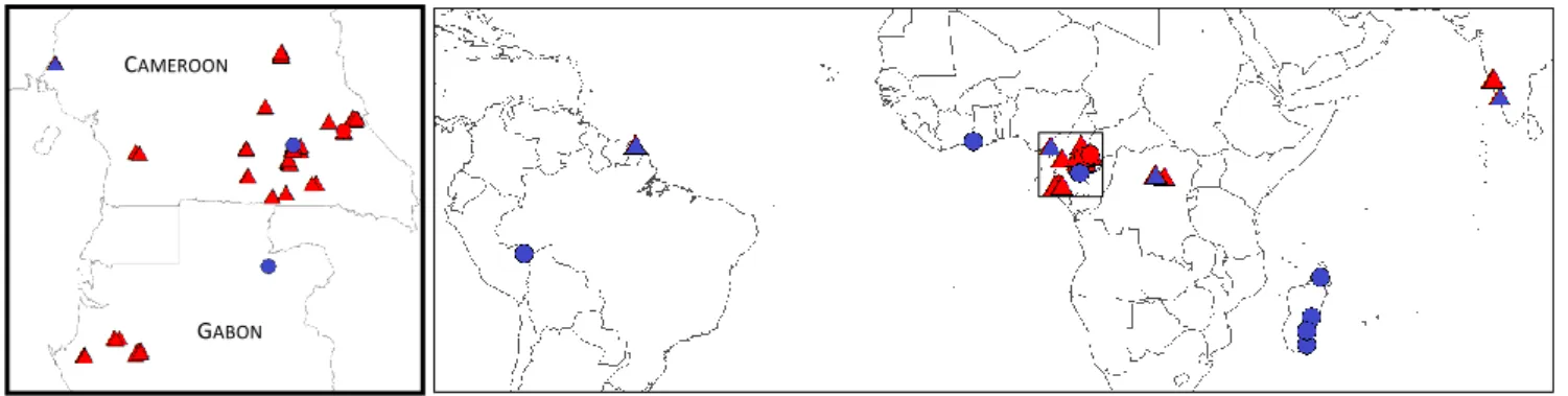
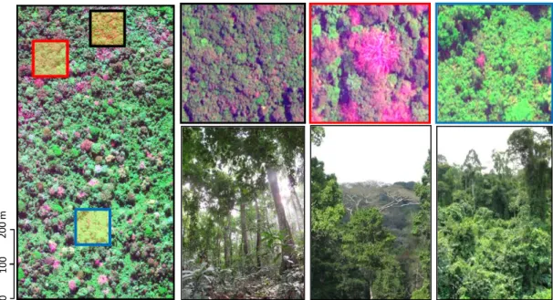
Core datasets of this work (at both tree- and plot-level) come from about five years of field data collection campaigns in central Africa (Cameroon, Gabon, Democratic Republic of Congo) carried out by the Institut de Recherche pour le Développement (IRD) in collaboration with the Ecole Normale Supérieure of Yaoundé I (LaBosystE, ENS, Université de Yaoundé I), the Missouri Botanical Garden (MBG) and the Université Libre de Kisangani (UniKis). During the two years preceding my thesis and during the thesis itself, I participated to the establishment of nearly 80 1-ha forest inventory plots, the bulk of which being located in south-eastern Cameroon (c. 50 %, left panel in Figure 1-3). Forests in this region have been described as a transitional type between evergreen and deciduous forests (Letouzey, 1985) and expand across the borders of neighboring countries. From a structural point of view, these forests can be described as forests mosaics that notably include patches of mixed, closed-canopy, semi-deciduous stands, open-canopy Marantaceae stands and monodominant

(Fayolle et al., 2016), and several logging companies are established in the region. Through a collaboration with the Alpicam company, we assembled a large destructive dataset on trees dimensions and AGB (77 trees).

Additional study areas

In the scope of this thesis, I investigate broad biophysical relationships, be it at the tree level in biomass allometry models or at the stand levels in canopy texture-based AGB models. In order to increase the robustness of the results, I compiled additional data from the literature, collaborating institutions or peer researchers (right panel on Figure 1-3).

The sets of 1 ha forest inventories from IRD and collaborators field work in central Africa were complemented with 28 1-ha plots from a forest-savanna mosaic in Republic Democratic of Congo (from Bastin et al., 2014), a 50 ha plots located in the Atlantic evergreen forests of western Cameroon (from Chuyong et al., 2004), 15 and 22 1-ha plots in evergreen and semi-deciduous forests of the Western Ghats of India (from Ploton et al., 2011 and Pargal et al., submitted) and 16 plots covering 85 ha of evergreen forests at Paracou, French Guiana (from Vincent et al., 2012). In total, texture analyses were based on 279 ha of forest inventory distributed on 3 continents.

To the 77 trees destructively sampled in south-eastern Cameroon, I added 132 trees from a semi-deciduous forest of the same region (from Fayolle et al., 2013), 99 trees sampled in a semi-semi-deciduous forest of Gabon (from Ngomanda et al., 2014), 29 trees sampled in an evergreen forest of Ghana (from Henry et al., 2010), 285 trees sampled in a dry-to-wet forest types gradient in Madagascar (from Vieilledent et al., 2012) and 51 trees sampled in an evergreen forest of Peru (from Goodman et al., 2014). The total destructive dataset (n=673) thus comprises trees from 6 sites distributed in five tropical countries (right panel in Figure 1-3).

Figure 1-3. Distribution of datasets across the tropics. Dots and triangles represent tree-level destructive datasets and field plot inventories, respectively. Red color indicates that data have been collected by IRD. Blue color indicates that data were compiled from literature, collaborating institutions or shared by the peer researchers.

CAMEROON

Figure 1-4. VHSR satellite image (GeoEye sensor) covering a typical forest mosaic from semi-deciduous forests of south-eastern Cameroon. Patches of Gilbertiodendron dewevrei (black square), mixed closed-canopy stands (red square) and open-canopy Marantaceae stands closely co-occur.

1.3.2 Sampling strategy and data description

Large trees exhibits the largest AGB variability at a given D and H while being insufficiently represented in biomass destructive datasets (Chave et al., 2005), probably because of the disproportionate amount of work that the biomass estimation of a large tropical canopy tree represents. To fill this gap, we exclusively targeted very large canopy trees in our field work protocol. This unique dataset, which was incorporated in the latest pantropical database (Chave et al. 2014), contains 17 out of the 30 world’s heaviest sampled tropical trees. For a typical tree, we measured the trunk diameter D, the tree height H and two perpendicular crown diameters before the tree was felled. After felling, tree biomass was estimated by combining direct measurements, indirect measurements and allometries. Direct measurements (i.e. weightings) were made on branches of varying sizes, to build an allometry relating branch diameter to biomass. We estimated the volume of the largest tree components (i.e. trunk and branches with diameter > 20 cm) by measuring diameters and lengths of approximately 2-m and 1-m long subsections along the trunk and branches, respectively. Biomass values were obtained by multiplying volumes by wood density estimates, derived from wood samples. The biomass of branches with D ≤ 20 cm was obtained with species-specific biomass allometries. A detailed description of the field protocol is provided in the supplementary material of chapter 2. An important feature of this dataset is that it contains a description of the crown geometry (from diameter and length measurements) and topology (from the identification of branching points), allowing to reconstruct the tree branching network (up to a branch diameter of c. 20 cm) in 3D and explore allometries and scaling properties at the branch level.

Destructive data compiled from other studies were obtained by direct biomass measurement, I refer the reader to the publications associated to each dataset for more details. Importantly, I only

0 100 2 0 0 m

Plot level data

Apart for plots at Paracou (85 ha) and Korup (50 ha), the sampling strategy at all sites was designed to optimize canopy texture analyses from VHSR optical images. In essence, 1 ha plots were distributed over a few hundred square kilometers (the typical footprint of a VHSR image) so to capture local diversity of forest stand types and ages. Measurement protocols deployed in central Africa, India and French Guiana were similar and consisted in describing the structure and composition of forest stands for all trees with D ≥ 10 cm. In addition to tree diameter at breast height (D), the description of stands structure included measurements of total tree height (H), trunk height (Ht) and crown diameter (Cd) on a subset of trees per plot (typically c. 50), to document local trees allometries. The identification of tree species allows retrieving species-level wood density estimates (

ρ)

1.4 Thesis outline

The thesis is structured into six chapters. The current chapter briefly depicts the scientific context and motivations of my doctoral study. It also includes the thesis research objectives, a description of the datasets and the thesis structure. A last section lists the publications I authored or co-authored on research topics related to the thesis subject.

In Chapter 2, I investigate how variations in tree form, with a particular focus on crown dimensions, influence the predictions (and error) of the pantropical biomass model. The analyses are based on the largest destructive dataset available to date that features information on tropical tree crown mass. After pinpointing the source of bias in the pantropical model, I propose an alternative model functional form. An original method for propagating tree biomass estimation error at the plot level is developed and highlights an interaction between forest structure and biomass model error, a source of uncertainty largely overlooked. This study was partly published in the journal Biogeosciences. In Chapter 3, I further explore the structural properties of large trees crowns that could explain the deviation between large trees biomass and the mathematical power form of the pantropical biomass model. An empirical assessment of MTE’s theoretical branch allometry is provided. A manuscript is in preparation from these results for the journal Trees – Structure and Function.

Chapter 4 presents the FOTO method, i.e. a remote sensing approach to retrieve forest structure and

biomass gradients from canopy texture features. I give a concise description of how the method works and the basic rationale behind it. Further, I provide a synthetic overview of the results obtained in separate empirical FOTO case studies on diverse forest ecosystems and from various remote sensing data types. This synthesis highlights methodological limits hindering the development of FOTO as a broad-scale, operational forest biomass monitoring method. This chapter was partly published in a book entitled Treetops at Risk (Springer).

Chapter 5 builds upon the synthesis in chapter 4. A simulation procedure is used, which includes the

representation of forest sample plots as three-dimensional mockups and the generation of virtual mockup canopy scenes. Simulated canopy scenes allow testing how the relation between texture features and stand biomass varies across forest types in a single, unified analysis frame (as opposed to previous empirical studies). The major limits identified in chapter 4 are addressed by complementing

FOTO texture with additional descriptors of forest stand structure, notably derived from lacunarity analysis. A ‘generalized’ biomass prediction model based on a combination of texture metrics is proposed, opening new perspectives for biomass retrieval from canopy texture at large scale. Part of these results was submitted for publication in Remote Sensing of Environment.

Finally, Chapter 6 presents the overall thesis discussion, focusing on the main contributions, limits and perspectives of this work.

1.5 List of (co-)publications

Estimation of biomass in forest sample plots

• Ploton, P., Barbier, N., Takoudjou Momo, S., Réjou-Méchain, M., Boyemba Bosela, F., Chuyong, G., Dauby, G., Droissart, V., Fayolle, A., Goodman, R.C., Henry, M., Kamdem, N.G., Mukirania, J.K., Kenfack, D., Libalah, M., Ngomanda, A., Rossi, V., Sonké, B., Texier, N., Thomas, D., Zebaze, D., Couteron, P., Berger, U., Pélissier, R., 2016. Closing a gap in tropical forest biomass estimation: taking crown mass variation into account in pantropical allometries. Biogeosciences 13, 1571–1585. doi:10.5194/bg-13-1571-2016

• Ploton, P., Barbier, N., Couteron, P., Momo, S.T., Griffon, S., Sonké, B., Uta, B., Pélissier, R. Assessing Da Vinci’s rule on large tropical tree crowns of contrasted architectures : evidence for area-increasing branching. In preparation for Trees – Structure and Function. • Picard, N., Rutishauser, E., Ploton, P., Ngomanda, A., Henry, M., 2015. Should tree biomass allometry be restricted to power models?

For. Ecol. Manag. 353, 156–163. doi:10.1016/j.foreco.2015.05.035

• Chave, J., Réjou-Méchain, M., Búrquez, A., Chidumayo, E., Colgan, M.S., Delitti, W.B.C., Duque, A., Eid, T., Fearnside, P.M., Goodman, R.C., Henry, M., Martínez-Yrízar, A., Mugasha, W.A., Muller-Landau, H.C., Mencuccini, M., Nelson, B.W., Ngomanda, A., Nogueira, E.M., Ortiz-Malavassi, E., Pélissier, R., Ploton, P., Ryan, C.M., Saldarriaga, J.G., Vieilledent, G., 2014. Improved allometric models to estimate the aboveground biomass of tropical trees. Glob. Change Biol. 20, 3177–3190. doi:10.1111/gcb.12629

Rational behind texture-based remote sensing methods

• Bastin, J.-F., Barbier, N., Réjou-Méchain, M., Fayolle, A., Gourlet-Fleury, S., Maniatis, D., de Haulleville, T., Baya, F., Beeckman, H., Beina, D., Couteron, P., Chuyong, G., Dauby, G., Doucet, J.-L., Droissart, V., Dufrêne, M., Ewango, C., Gillet, J.F., Gonmadje, C.H., Hart, T., Kavali, T., Kenfack, D., Libalah, M., Malhi, Y., Makana, J.-R., Pélissier, R., Ploton, P., Serckx, A., Sonké, B., Stevart, T., Thomas, D.W., De Cannière, C., Bogaert, J., 2015c. Seeing Central African forests through their largest trees. Sci. Rep. 5, 13156. doi:10.1038/srep13156

• Blanchard, E., Birnbaum, P., Ibanez, T., Boutreux, T., Antin, C., Ploton, P., Vincent, G., Pouteau, R., Vandrot, H., Hequet, V., 2016. Contrasted allometries between stem diameter, crown area, and tree height in five tropical biogeographic areas. Trees 1–16. • Jucker, T., Caspersen, J., Chave, J., Antin, C., Barbier, N., Bongers, F., Dalponte, M., van Ewijk, K.Y., Forrester, D.I., Haeni, M., Higgins,

S.I., Holdaway, R.J., Iida, Y., Lorimer, C., Marshall, P.L., Momo, S., Moncrieff, G.R., Ploton, P., Poorter, L., Rahman, K.A., Schlund, M., Sonké, B., Sterck, F.J., Trugman, A.T., Usoltsev, V.A., Vanderwel, M.C., Waldner, P., Wedeux, B.M.M., Wirth, C., Wöll, H., Woods, M., Xiang, W., Zimmermann, N.E., Coomes, D.A., 2016. Allometric equations for integrating remote sensing imagery into forest monitoring programmes. Glob. Change Biol. doi:10.1111/gcb.13388

Estimation of biomass from canopy texture features

• Ploton, P., Pélissier, R., Barbier, N., Proisy, C., Ramesh, B.R., Couteron, P., 2013. Canopy texture analysis for large-scale assessments of tropical forest stand structure and biomass, in: Treetops at Risk. Springer, pp. 237–245.

• Ploton, P., Barbier, N., Couteron, P., Ayyappan, N., Antin, C.M., Bastin, J.-F., Chuyong, G., Dauby, G., Droissart, V., Gastellu-Etchegorry, J.-P., Kamdem, N.G., Kenfack, D., Libalah, M., Momo, S., Pargal, S., Proisy, C., Sonké, B., Texier, N., Thomas, D., Zebaze, D., Verley, P., Vincent, G., Berger, U., Pélissier, R. Combining canopy texture metrics from optical data to retrieve tropical forest aboveground biomass in complex forest mosaics. Submitted to Remote Sensing of Environment.

• Ploton, P., Pélissier, R., Proisy, C., Flavenot, T., Barbier, N., Rai, S.N., Couteron, P., 2012. Assessing aboveground tropical forest biomass using Google Earth canopy images. Ecol. Appl. 22, 993–1003. doi:10.1890/11-1606.1