The mixed p-spin model : selecting, following and losing states

(1)

HAL Id: tel-02883385

https://tel.archives-ouvertes.fr/tel-02883385

Submitted on 29 Jun 2020

HAL is a multi-disciplinary open access archive for the deposit and dissemination of sci-entific research documents, whether they are pub-lished or not. The documents may come from teaching and research institutions in France or abroad, or from public or private research centers.

L’archive ouverte pluridisciplinaire HAL, est destinée au dépôt et à la diffusion de documents scientifiques de niveau recherche, publiés ou non, émanant des établissements d’enseignement et de recherche français ou étrangers, des laboratoires publics ou privés.

states

Giampaolo Folena

To cite this version:

Giampaolo Folena. The mixed p-spin model : selecting, following and losing states. Disordered Systems and Neural Networks [cond-mat.dis-nn]. Université Paris-Saclay; Università degli studi La Sapienza (Rome), 2020. English. �NNT : 2020UPASS060�. �tel-02883385�

(2)

Thè

se

d

e

doctorat

NNT : 2020UP ASS060

The mixed

p

-spin model:

selecting, following and losing states

Thèse de doctorat de l’Université Paris-Saclay et de "La Sapienza" Università di Roma

École doctorale n 564, Physique en Île-de-France (PIF)

Spécialité de doctorat: Physique

Unité de recherche: Université Paris-Saclay, CNRS, LPTMS, 91405, Orsay, France

Référent: Faculté des sciences

Thèse présentée et soutenue à Rome, le 10 mars 2020, par

Giampaolo FOLENA

Composition du jury:

Luca LEUZZI Président

Directeur de Recherche, CNR-Nanotec, Roma (IT)

Chiara CAMMAROTA Rapporteur

Maître de Conférences (HDR), King’s College, London (GB)

Patrick CHARBONNEAU Rapporteur

Professeur Associé, Duke University, Durham (USA)

Florent KRZAKALA Examinateur

Professeur, Sorbonne Université, Paris

Luca DALL’ASTA Examinateur

Professeur Associé, Politecnico di Torino (IT)

Pierfrancesco URBANI Examinateur Chargé de Recherche, IPhT, CEA/Saclay

Silvio FRANZ Directeur

Professeur des Universités, LPTMS, Orsay

Federico RICCI-TERSENGHI Codirecteur Professeur, "La Sapienza", Università di Roma (IT)

(3)

Anecdote: this thesis has been discussed in Rome on the 10 of March 2020, one day after the italian national lockdown and one day before the declaration of

(4)

Thesis Summary - English

The main driving notion behind my thesis research is to explore the connection between the dy-namics and the static in a prototypical model of glass transition, i.e. the mean-field p-spin spherical model. This model was introduced more than 30 years ago with the purpose of o↵ering a simplified model that had the same equilibrium dynamical slowing down, theoretically described a few years earlier by mode-coupling theory. Over the years, the p-spin spherical model has shown to be a very meaningful and promising model, capable of describing many equilibrium and out-of-equilibrium aspects of glasses. Eventually it came to be considered as a prototypical model of glassiness. Having such a simple but rich reference model allows a coherent examination of a subject, in our case the glass behavior, which presents a very intricate phenomenology. Thus, the main purpose is not to have a quantitative prediction of the phenomena, but rather a broader view with a strong analytical basis. In this sense the p-spin model has assumed a role for disordered systems which is comparable to that of the Ising model for understanding ferromagnetism. My research is a natural path to reinforce our knowledge and comprehension of this model.

In the first chapter, we provide a general introduction to supercooled liquids and their phe-nomenology. The introduction is brief, and the main goal is to give a general overview, mainly from the point of view of the Random First Order Transition, while considering other perspectives on the subject and attempting to provide a ‘fair’ starting bibliography to whomever wants to study supercooled liquids. The last section focuses on the Potential Energy Landscape paradigm (PEL), which in my view, gives a very solid modelization of glassy phenomenology, and shares many aspects with mean-field analysis.

In the second chapter, the p-spin spherical model is presented in details. The equilibrium analysis is performed with the replica formalism, with a focus on the ultrametric structure. Then, di↵erent tools to study its free energy landscape are introduced: the TAP approach, the Franz-Parisi potential and the Monasson method. These three di↵erent ways of selecting states are carefully contrasted and their analogies and di↵erences are underlined, in particular highlighting the di↵erent behavior played by pure and mixed p-spin models. Then the equilibrium dynamics is discussed, and a selection of classical results on the dynamical slowing down are analyzed by numerical integration. To conclude, the out-of-equilibrium dynamics in the two temperature protocol is analyzed. This shows two di↵erent regimes, the state following and the aging. For both, an asymptotic analysis and a numerical integration are performed and compared. A strong emphasis is given to the possibility of describing the asymptotic dynamics with a static potential.

The third chapter presents all the new results that emerged during my research. The study fo-cuses on the two temperature protocol, starting in equilibrium and setting the second temperature to zero, which corresponds to a gradient descent dynamics. This protocol is especially interesting because it corresponds to the search of inherent structure of the energy landscape. The integrated dynamics, depending on the starting temperature, shows three di↵erent regimes, one that corre-sponds to a new phase, which shows aging together with memory of the initial condition. This new phase is not present in pure p-spin models, only in mixed ones. In order to theoretically describe this new phase, a constrained analysis of the stationary points of the energy landscape is performed. A numerical simulation of the system is also presented to confirm this new scenario.

(5)

R´

esum´

e de la Th`

ese - Fran¸cais

L’objectif principal de cette thèse est d’explorer le lien entre la dynamique et la statique dans un modèle prototypique de transition vitreuse, i.e. le modèle à champ moyen du p-spin sphérique. Ce modèle a été introduit il y a plus de 30 ans dans le but d’o↵rir un modèle simplifié ayant, à l’équilibre, le même ralentissement dynamique décrit théoriquement quelques années plus tôt par la théorie des modes couplés. Au fil des ans, le modèle du p-spin sphérique s’est révélé être un modèle très significatif et prometteur, capable de décrire de nombreux aspects d’équilibre et hors équilibre des verres. Avoir un tel modèle de référence simple mais riche permet un examen cohérent d’un sujet, dans notre cas le comportement du verre qui présente une phénoménologie très complexe. Ainsi, le but principal n’est pas d’avoir une prédiction quantitative des phénomènes, mais plutôt une vue plus large avec une forte base analytique. En ce sens, le modèle du p-spin a assumé un rôle pour les systèmes désordonnés qui est comparable à celui du modèle Ising pour comprendre le ferromagnétisme. Ma recherche est une voie naturelle pour renforcer notre connaissance et notre compréhension de ce modèle.

Dans le premier chapitre, nous donnons une introduction générale aux liquides surfondus et leur phénoménologie. L’introduction est brève, et l’objectif principal est de donner un aper¸cu général, principalement du point de vue de la transition aléatoire du premier ordre, tout en tenant compte d’autres points de vue sur le sujet et en essayant de fournir une ‘bonne’ bibliographie de départ à quiconque veut étudier les liquides surfondus. La dernière section se concentre sur le paradigme du surface d’énergie potentielle (PEL), qui, à mon avis, donne une modélisation très solide de la phénoménologie vitreuse, et partage de nombreux aspects avec l’analyse du champ moyen.

Dans le deuxième chapitre, le modèle du p-spin sphérique est présenté en détail. L’analyse d’équilibre est réalisée avec le formalisme des répliques, avec un accent sur la structure ultramétrique. Ensuite, di↵érents outils pour étudier son paysage d’énergie libre sont présentés: l’approche TAP, le potentiel de Franz-Parisi et la méthode de Monasson. Ces trois manières di↵érentes de sélectionner les états sont soigneusement contrastées et leurs analogies et di↵érences sont soulignées, en partic-ulier le comportement di↵érent joué par les modèles du p-spin purs et mixtes. Ensuite, la dynamique d’équilibre est discutée, et une sélection de résultats classiques sur le ralentissement dynamique sont analysés par intégration numérique. Pour conclure, la dynamique hors équilibre dans le protocole à deux températures est analysée. Cela montre deux régimes di↵érents, des états suivables et du vieil-lissement. Pour les deux, une analyse asymptotique et une intégration numérique sont e↵ectuées et comparées. L’accent est mis sur la possibilité de décrire la dynamique asymptotique avec un potentiel statique.

Le troisième chapitre présente tous les nouveaux résultats qui ont émergé au cours de mes recherches. L’étude se concentre sur le protocole à deux températures, commen¸cant à l’équilibre et fixant la deuxième température à zéro, ce qui correspond à une dynamique de descente du gradi-ent. Ce protocole est particulièrement intéressant car il correspond à la recherche de la structure inhérente du paysage énergétique. La dynamique intégrée, en fonction de la température de départ, montre trois régimes di↵érents. Une de ceux-ci corresponde à une nouvelle phase, qui présente le vieillissement avec la mémoire de la condition initiale. Cette nouvelle phase n’est pas présente dans les modèles du p-spin pure, seulement dans les modèles mixtes. Afin de décrire théoriquement cette nouvelle phase, une analyse des points stationnaires du paysage énergétique est e↵ectuée. Une simulation numérique du système est également présentée pour confirmer ce nouveau scénario.

(6)

Riassunto della Tesi - Italiano

L’obiettivo principale di questa tesi è di esplorare il legame tra la dinamica e la statica in un modello prototipico di transizione vetrosa, i.e. il modello di campo medio del p-spin sferico. Questo modello è stato introdotto più di 30 anni, come modello prototipico per il rallentamento critico all’equilibrio, quale era stato descritto alcuni anni prima dalla teoria dei modi accoppiati. Nel corso degli anni, il modello del p-spin sferico si è rivelato molto pregnante, capace di descrivere diversi aspetti dei vetri, sia all’equilibrio che fuori dall’equilibrio. Avere un simile modello di riferimento, semplice ma ricco, permette un esame coerente di un soggetto, quale è il comportamento dei vetri, con una fenomenologia molto complessa. Lo scopo principale non è quello di avere una previsione quantitativa dei fenomeni, ma piuttosto una visione più ampia con una forte base analitica. In questo senso, il modello del p-spin ha assunto un ruolo per i sistemi disordinati che è paragonabile a quello del modello di Ising per il ferromagnetismo. La mia ricerca è volta a ra↵orzare la nostra conoscenza e comprensione di questo modello.

Nel primo capitolo è fornita un’introduzione generale ai liquidi sopra↵usi e alla loro fenomenolo-gia. L’introduzione è breve, e l’obiettivo principale è quello di fornire una panoramica generale, soprattutto dal punto di vista della transizione disordinata del primo ordine (RFOT), pur tenendo conto di altri punti di vista sul soggetto e cercando di fornire una ‘buona’ bibliografia di partenza a chiunque voglia studiare i liquidi sopra↵usi. L’ultima sezione si concentra sul paradigma della superficie di energia potenziale (PEL), che, a mio parere, fornisce una modellazione molto solida della fenomenologia vetrosa, e condivide molti aspetti con l’analisi di campo medio.

Nel secondo capitolo è presentato in dettaglio il modello del p-spin sferico. L’analisi dell’equilibrio è realizzata con il formalismo delle repliche, con un accenno alla struttura ultrametrica. Vengono poi presentati vari strumenti per studiare il paesaggio di energia libera: l’approccio TAP, il poten-ziale di Franz-Parisi e il metodo di Monasson. Questi tre diversi modi di selezionare gli stati sono accuratamente confrontati e le loro analogie e di↵erenze sono messe in evidenza, in particolare il diverso comportamento dei modelli di p-spin puri e misti. Poi viene discussa la dinamica di equi-librio, e alcuni risultati classici sul rallentamento dinamico sono analizzati attraverso l’integrazione numerica della dinamica. In conclusione, si analizza la dinamica fuori dall’equilibrio nel protocollo a due temperature. Questo mostra due diversi regimi dinamici, di inseguimento degli stati e di invecchiamento. In entrambi i casi, sono e↵ettuate e confrontate l’analisi asintotica e l’integrazione numerica. L’accento è posto sulla possibilità di descrivere la dinamica asintotica attraverso un potenziale statico.

Il terzo capitolo presenta i nuovi risultati emersi nel corso della mia ricerca. Lo studio si con-centra sul protocollo a due temperature, iniziando dall’equilibrio e fissando la seconda temperatura a zero, il che corrisponde ad una dinamica di discesa del gradiente. Questo protocollo è particolar-mente interessante perché corrisponde alla ricerca delle strutture inerenti nel paesaggio energetico. Questa dinamica, in funzione della temperatura di partenza, mostra tre di↵erenti regimi. Uno di questi corrisponde ad una nuova fase, che presenta invecchiamento insieme alla memoria della con-dizione iniziale. Questa nuova fase non è presente nei modelli di p-spin puro, ma solo nei modelli misti. Per descrivere teoricamente questa nuova fase, si e↵ettua un’analisi dei punti stazionari del paesaggio energetico. Inoltre, per confermare questo nuovo scenario, viene presentata una simu-lazione numerica del sistema.

(7)

(8)

(9)

Introduction 1

1 Glass Transition 5

1.1 Super-Cooled Liquids . . . 5

1.1.1 Equilibrium Regimes . . . 7

1.1.2 Statical vs Dynamical Signatures . . . 10

1.2 Potential Energy Landscape . . . 18

1.2.1 Inherent Structures Partitioning . . . 18

1.2.2 The Gaussian PEL Approximation . . . 21

2 Prototypical model of Supercooled Liquid 29 2.1 The p-spin spherical model . . . 29

2.1.1 A short History . . . 29

2.1.2 The Model . . . 30

2.1.3 Replica Trick . . . 31

2.1.4 The Replicated Free Energy . . . 32

2.1.5 Replica Symmetric Ansatz . . . 34

2.1.6 One Step of Replica Symmetric Breaking . . . 37

2.1.7 k-RSB Solution . . . 39

2.2 Following States . . . 50

2.2.1 Following Energy Minima . . . 50

2.2.2 Following Equilibrium States . . . 53

2.3 Counting States . . . 62

2.3.1 Counting Energy Minima . . . 62

2.3.2 Counting with a Legendre Transform . . . 66

2.3.3 Universal Complexity . . . 70

2.4 Three ways of Selecting States . . . 72

2.4.1 Pure Models: Perfect Matching . . . 72 vii

(10)

2.4.2 Mixed Models: which States are Selected? . . . 75

2.5 Mean Field Dynamical Equations with Cavity Method . . . 78

2.5.1 Equilibrium Equations . . . 80

2.5.2 Equations for Correlation and Response . . . 81

2.5.3 Out-of-equilibrium: two Temperature Protocol . . . 82

2.6 Equilibrium Dynamics . . . 84

2.7 Out of Equilibrium Dynamics . . . 91

2.7.1 Two Temperature Protocol: Following States . . . 91

2.7.2 Two Temperature Protocol: Aging . . . 94

2.7.3 Two Temperature Protocol: Static V SDynamics . . . 101

2.7.4 Two Temperature Protocol: “Classical” Aging . . . 101

3 Exploring the Landscape through Gradient Descent 105 3.1 Numerical Integration . . . 105

3.1.1 Under-threshold Dynamics . . . 106

3.1.2 Relaxing on a Marginal Manifold . . . 107

3.1.3 Aging in a Confined Space . . . 109

3.1.4 Onset Temperature a Semi-empirical Law . . . 112

3.1.5 Two Time Scales for Two Power Laws . . . 114

3.2 Constrained Complexity . . . 118

3.3 Numerical Simulation . . . 123

3.3.1 Dilution . . . 123

3.3.2 Annealing V SPlanting . . . 125

3.3.3 Simulation V SIntegration . . . 129

3.4 The Emergence of a New Phase . . . 132

Perspectives 135 A Appendices 139 A.1 Gaussian Correlation of Disorder . . . 139

A.1.1 The typical Hessian belongs to the GOE . . . 140

A.2 k-RSB q-extremization . . . 142

A.3 Algebra of Overlap Matrices . . . 143

A.3.1 Derivatives . . . 143

A.3.2 Algebra of RS Matrices . . . 143

A.4 TAP Free Energy . . . 144

A.5 A Toy Model with Memory from the Ergodic Phase . . . 148

A.6 Equilibrium Integration . . . 150

(11)

A.7.1 Fixed-step Algorithm . . . 153

A.7.2 Rescaling Algorithm . . . 154

A.7.3 Structure and Approximations . . . 154

A.7.4 Simple Aging . . . 157

A.7.5 Limits and Errors . . . 157

A.8 Formulario p-spin . . . 159

(12)

Details that could throw doubt on your interpretation must be given, if you know them. You must do the best you can – if you know anything at all wrong, or possibly wrong – to explain it. If you make a theory, for example, and advertise it, or put it out, then you must also put down all the facts that disagree with it, as well as those that agree with it.

(13)

The main driving notion behind my thesis research is to explore the connection be-tween the dynamics and the static in a prototypical model of glass transition, i.e. the mean-field p-spin spherical model. This model was introduced more than 30 years ago with the purpose of o↵ering a simplified model that had the same equilibrium dynamical slowing down, theoretically described a few years earlier by mode-coupling theory. Since its birth, statistical mechanics has always searched in the static analysis of some ‘carefully’ defined landscape; a path to avoid impossible dynamical calcu-lations. One first fundamental concept is the idea of mapping temporal averages of observables into measures over phase space. This approach has allowed us to attain many fundamental relations between equilibrium observables. The same emphasis, in identifying the ensemble of dynamical paths in a static measure, continues to nourish the spirit of many researchers, and has been the drive all along my PhD research.

Over the years, the p-spin spherical model has shown to be a very meaningful and promising model, capable of describing many equilibrium and out-of-equilibrium as-pects of glasses. Eventually it came to be considered as a prototypical model of glassiness. Having such a simple but rich reference model allows a coherent exam-ination of a subject, in our case the glass behavior, which presents a very intricate phenomenology. Thus, the main purpose is not to have a quantitative prediction of the phenomena, but rather a broader view with a strong analytical basis. In this sense the p-spin model has assumed a role for disordered systems which is compara-ble to that of the Ising model for understanding ferromagnetism. My research is a natural path to reinforce our knowledge and comprehension of this model.

Over my three years of PhD research, I have concentrated on the out-of-equilibrium phenomenology of p-spin models, and in particular on a specific, two temperature protocol: a system prepared at one temperature and relaxed at another one. In the study of this out-of-equilibrium dynamics some unexpected phenomena were

(14)

ered, which revealed a new interesting path of research and added a new brick to this prototypical structure of glassiness. In particular, we can assert now with certainty that there is no absolute threshold in the energy landscape of mean-field models. The region of phase space asymptotically explored by the dynamics depends on the chosen cooling path from high temperature. This was already known for finite-dimensional models, but not for mean-field ones. This new observation questions some paradigms that were built because of a pathological symmetry, present only in a subclass of these models, i.e., pure models.

In our attempt to understand this new unexpected behavior, my supervisors and me, have tackled the problem from many di↵erent angles; from the numerical integration of the long-time dynamics to the analytical study of the asymptotic dynamics, from the numerical simulation of finite-size systems to the theoretical study of the energy landscape. All these studies have clarified the origin of this anomalous behavior, and in particular, the parallelism aforementioned between static and dynamics. The major result of this work has been to introduce a new out-of-equilibrium mean-field phase and to characterize it in great detail.

In the first chapter, we provide a general introduction to supercooled liquids and their phenomenology. The introduction is brief, and the main goal is to give a general overview, mainly from the point of view of the Random First Order Transition, while considering other perspectives on the subject and attempting to provide a ‘fair’ starting bibliography to whomever wants to study supercooled liquids. The last section focuses on the Potential Energy Landscape paradigm, which in my view, gives a very solid modelization of glassy phenomenology, and shares many aspects with mean-field analysis.

In the second chapter, the p-spin spherical model is presented in details. The equilibrium analysis is performed with the replica formalism, with a focus on the ultrametric structure. Then, di↵erent tools to study its free energy landscape are in-troduced: the TAP approach, the Franz-Parisi potential and the Monasson method. These three di↵erent ways of selecting states are carefully contrasted and their analo-gies and di↵erences are underlined, in particular highlighting the di↵erent behavior played by pure and mixed p-spin models. Then the equilibrium dynamics is discussed, and a selection of classical results on the dynamical slowing down are analyzed by numerical integration. To conclude, the out-of-equilibrium dynamics in the two tem-perature protocol is analyzed. This shows two di↵erent regimes, the state following and the aging. For both, an asymptotic analysis and a numerical integration are performed and compared. A strong emphasis is given to the possibility of describing the asymptotic dynamics with a static potential.

(15)

The study focuses on the two temperature protocol, starting in equilibrium and setting the second temperature to zero, which corresponds to a gradient descent dynamics. This protocol is especially interesting because it corresponds to the search of inherent structure of the energy landscape (PEL perspective). The integrated dynamics, depending on the starting temperature, shows three di↵erent regimes, one that corresponds to a new phase, which shows aging together with memory of the initial condition. This new phase is not present in pure p-spin models, only in mixed ones. In order to theoretically describe this new phase, a constrained analysis of the stationary points of the energy landscape is performed. A numerical simulation of the system is also presented to confirm this new scenario.

I wish to remark that all the thesis has been written with the continuous attention of providing my personal view over each subject. Therefore, sometimes things are not presented in a customary way, but I hope that this can stimulate a further understanding of the subject matter.

(16)

(17)

Glass Transition

1.1 Super-Cooled Liquids

A supercooled liquid is a liquid followed down to temperatures at which the crystal would be the stable phase. It is possible to follow this metastable branch if the cooling is fast enough so that the characteristic time to nucleate the crystal is much larger than the equilibrium relaxation time of the supercooled liquid (SCL). If this is the case, the SCL can be followed down in temperature until it starts to develop a fast increase of the relaxation time, such that it is no longer possible to equilibrate it on an experimental time scale ⌧exp, thus the observed system is out of equilibrium. This

marks the temperature Tg at which the “non-equilibrated” SCL is considered a glass.

Conventionally Tghas been fixed to the temperature at which the viscosity overcomes

the threshold ⌫g = 1013 Poise⇤. This convention however is ‘dangerous’ because the

temperature at which the system gets out of equilibrium strictly depends on the

protocol used to prepare it. The glass is a memorius phase of matter†_{. In a normal}

phase of matter physical properties are uniquely defined by a small set of intensive variables (T, P, ...), while each glass has its own properties, depending on how it has been prepared. This is very clear when thinking of commercial silica-based glasses. The dependence on the preparation protocol is closely related to the way in which the system has gone out of equilibrium, which in turn is connected to the experimental time scale considered. Therefore the properties of the glass depend on the time scale

at which we observe it. Waiting for an incredibly long time ⌧SCL the system is expect

to relax to the equilibrium underlying SCL. And by waiting for an even longer period

⇤_{which corresponds to relaxation times of the order of 10-100s for molecular and atomic glass} formers

†_{if it can be defined so}

(18)

entr opy temperature SCL∼10-13 SCL∼10-9 SCL∼103 TMCT Tg Ton TK crystal liquid SCL glasses exp cry∼1020 SCL∼1010

Figure 1.1: (left): idealized plot of entropy vs temperature in a SCL and in the relative crystal. The arrow highlights the enormous di↵erence in time scales⌧exp⌧ ⌧SCL ⌧ ⌧cry when the system gets out of equilibrium (right): dynamic susceptibility of o-terphenyl as a function of frequency, with di↵erent relaxations regimes highlighted. [Pet+13],

of time ⌧crythe system should find the really stable crystalline phase. Each relaxation

time is expected to depend on some activated dynamics (nucleation-type). As long

as ⌧exp ⌧ ⌧SCL ⌧ ⌧cry the glass is “well defined” and its properties depend on its

history and in particular on the path it has been driven through, in the space of intensive variables, from the point it has fallen out-of-equilibrium (⌧exp ⇡ ⌧SCL).

From this discussion the difficulties in building a theory that embodies all this history dependence should appear clear. As it is custom in statistical mechanics, such a theory should transform the average over dynamical path into a measure upon the phase space, which at equilibrium is the well known Boltzmann-Gibbs

distribution (e H_{). One of the main foci of this thesis is to build such a measure}

for a two-temperatures protocol: a quench from an initial temperature T0 _{to a final}

temperature T .

In the following sections, in order to elucidate the major peculiarities of SCL we will follow the perspective of random first order transition RFOT, which drives all the modelization from a mean-field viewpoint (see [BB09] for a comprehensive re-view). We will simplify as much as possible the discussion and not introduce spatial description if not indispensable - even hough in recent years spatial and temporal heterogeneities have acquired an essential role in the description of ‘glassiness’ [Edi00; Ber11]. For the interested reader a plethora of very interesting reviews about SCL are available, each one with its theoretical background dependent on the commu-nity of reference. For a very brief and in-depth panorama of the glass transition

(19)

[DS01; Cha+14a]. From the MCT perspective [GS92]. For a short and dense review of RFOT [LW07]. For a pedestrian introduction to SCL with a RFOT-replica per-spective [Cav09]. For a perper-spective RFOT closer to the numerical results [BB11]. To focus only on the dynamical (and not thermodynamical) description of the glass transition[CG10]. For a question-answer experimental point of view [Ang+00c]. For other experimental perspectives [Dyr06; EH12]. For an introduction to the Potential Energy Landscape paradigm [Sci05]. For a very detailed analysis of PEL [Heu08]. For a theoretical focus towards out-of-equilibrium dynamics [Cug02].

1.1.1 Equilibrium Regimes

We wish here to sketch the equilibrium regimes of a SCL, upon changing temper-ature T . In the following we use s to denote a configuration in phase space. This configuration evolves following a Hamiltonian dynamics. One very e↵ective observ-able to characterize this dynamics - in and out-of-equilibrium - is the overlap of the

configuration at a time t0 with the configuration at a subsequent time t:

C(t, t0) = s(t)· s(t0) (1.1)

where · is a scalar product in phase space. This correlation function gives a

di-rect characterization of di↵erent regimes and phases of matter. The system is at equilibrium if:

C(t, t0) = C(t t0) (1.2)

together with the fact there is no energy flux in and out of the system, i.e. fluctuation dissipation theorem (FDT) holds. The system is ergodic if:

lim

t!0C(t) = 0 (1.3)

At equilibrium, an ergodic SCL is in the liquid phase, while a non-ergodic SCL is considered in the glassy phase.

Given this observable, let’s sketch what happens to a SCL starting from high temperatures (a cartoon of the transition is shown in figure 1.2.1). Above a

so-called onset temperature Ton the equilibrium SCL is ergodic and a fast exponential

relaxation occurs:

C(t)_{/ exp( t/⌧}↵)) ⌧↵ / exp(T 1) (1.4)

where ⌧↵ is the relaxation time of the system and follows an Arrhenius law. In this

regime the kinetic energy dominates.

Around Tonthe system starts feeling the presence of the energy landscape, kinetic

(20)

dynamics decouples into two di↵erent regimes, ↵-relaxation (slow) and -relaxation (fast), which in terms of the correlation C(t) signifies the development of a plateau. This is often described as a “cage forming” behavior. On short time scale ⌧ each constituent of the system is trapped in a cage and experiences a fixed landscape. On

another time scale ⌧↵ the cages deform and the system di↵uses. At this point the

role of the observation ⌧exp time in the modelization of the system starts to become

appreciable. In fact if ⌧ ⌧ ⌧exp ⌧ ⌧↵ the system can be considered a fully-fledged

glass.

Going down in temperature the largest time scale ⌧↵ diverges with a power-law

and the correlation C(t) shows a critical behavior in the development of a plateau:

C(t)_{' (t/⌧ )} a+ qM CT ⇠ qM CT (t/⌧↵)b ⌧↵ / (T TM CT) (1.5)

where a, b are the exponents that govern the approach to and the depart from the plateau, respectively. All this behavior is predicted by the mode coupling theory

(MCT)⇤ (see [RC05] for a review). This is a critical theory and for this reason

it has some sort of universality, however it ignores activated events which occur

before reaching TM CT. Thus in finite dimensional systems TM CT flags a crossover

region, which, in the extreme case of mean-field models (fully connected, infinite dimensional,...), becomes a sharp thermodynamic transition that separates the SCL from glass states. In finite dimensional systems, however, no metastable state is well defined because activated events are always possible with finite probability and the

system can di↵use from one pseudo-glass to another†_{. While there is one ergodic SCL,}

there exist many (pseudo-)glasses, which in mean-field correspond to metastable

states. The logarithm of their number Sc is extensive, it is called ‘configurational

entropy’ and it goes linearly to zero at a finite temperature TK, the Kauzmann

temperature.

Further decreasing the temperature below TM CT, the system keeps ergodic but the

divergence of the time scale ⌧↵ then scales as:

⌧↵ / exp( F ) ⇡ exp( d/Sc✓)1/(d ✓) ⇡ (T TK)

✓/(d ✓) _(1.6)

where is the surface tensions between pseudo-glasses. Thus the relaxation

dy-namics is directly connected to the structure of free energy landscape through the configurational entropy. Behind this prediction lies a nucleation ‘argument’, which in the literature is dubbed “mosaic picture” (see section 1.1.2). Glasses nucleate inside

⇤_{each exponent is given by the theory}

†_{‘pseudo-glass’ is obtained whenever one considers the short time dynamics below T}

M CT in a real system

(21)

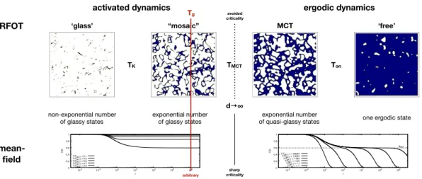
exponential number of quasi-glassy states exponential number

of glassy states one ergodic state

non-exponential number of glassy states Ton TMCT TK “mosaic” MCT ‘free’ ‘glass’

activated dynamics ergodic dynamics

0 0.2 0.4 0.6 0.8 1 10-4 10-2 100 102 104 106 108 C(t ) t T/TMCT= 0.1 T/TMCT= 0.3 T/TMCT= 0.5 T/TMCT= 0.7 T/TMCT= 0.9 RFOT mean-field avoided criticality d→∞ sharp criticality 0 0.2 0.4 0.6 0.8 1 10-4 10-2 100 102 104 106 108 qMCT C(t ) t T/TMCT= 1.00001 T/TMCT= 1.0001 T/TMCT= 1.001 T/TMCT= 1.01 T/TMCT= 1.1 T/TMCT= 1. Tg arbitrary

Figure 1.2: Random First Order Transition stems from the perspective that the real ‘glass’ can be described around an underlying mean-field core

glasses and the plateau continue to elongate. The mosaic picture is the most de-bated and weakest part of the RFOT perspective, but it continues to be stringently supported since it is powered by a strong mean-field core. One of the strongest mathematical prediction of mean-field in this temperature region is the partitioning

of the phase space in many ‘well separated’ basins ⇤ _{which gives a total free energy}

partitioned in a ‘large’ number of states S :

F = log⇣ X S X s2S e H[s]⌘= log⇣ X S e fS ⌘ = log⇣ Z df e f +Sc(f )⌘ _(1.7)

which, in mean-field models, is dominated by the saddle point @fSc(f⇤) = , which

is analogous to the equilibrium relation @ES(E⇤) = , but at the level of states S .

We see that the temperature T plays the role of an equilibrium parameter (Legendre transform) at two di↵erent scales. Inside basins the temperature is what defines the thermal bath perceived at a configuration level and between basins it regulates the exchange of free energy. This suggests an abstract interpretation of the decoupling of time scales described at the level of the correlations.

Below TK, the dynamics is non-ergodic also for a real system, at least with the

RFOT perspective. At TK there is a true thermodynamic transition, below which

phase space is ergodically broken and the system is confined into one of many glassy state. However, given the nature of the transition there is no direct way to verify

(22)

this prediction. Whether the glass formation is a purely dynamical e↵ect or the result of an underlying static transition is far from understood, but following the

Occam’s razor principle, RFOT⇤ _{has for now all the ingredients to be considered a}

‘good candidate’ to describe the SCL phenomenology.

1.1.2 Statical vs Dynamical Signatures

In this section we briefly overview the main theoretical interpretation and experi-mental observations concerning the aforementioned temperatures TK, TM CT, Ton which

constitute the backbone of RFOT interpretation. For each temperature a brief his-torical account will be presented together with some di↵erent theoretical perspective on the transition, with a particular emphasis on the contrast between statical and dynamical perspectives.

The Onset Temperature

The onset temperature Ton† marks the passage from uncorrelated dynamics above

to the “landscape dominated dynamics” below. It is a ‘quite sharp’ crossover that appears in a variety of materials, such as molecular liquids, colloids, metallic liquids... [Wee+00; Sas02; Jai+16]. And it has been studied in many numerical simulations

[KA95a; SDS98; Sas00; Sin+12; Ban+17]. Above Ton the characteristic relaxation

time of the system follows an Arrhenius law and two times observables presents an exponential decay:

⌧↵ / exp(T 1) C(t)/ exp( t/⌧↵) (1.8)

Below Ton cooperative behavior between constituents of the system begins which find

the way to continue their motion while in a very crowded environment. This deep change can be seen in many di↵erent aspects. First the deviation from the Arrhenius law and the stretching of the exponential relaxations‡_:

⌧↵ 6/ exp(T 1) C(t)/ exp

⇣

(t/⌧↵)

⌘

(1.9)

where _{2 [0, 1] is a stretching exponent that decreases with temperature. Another}

very crucial aspects is the decoupling of time scales ⌧↵ and ⌧ , respectively the scale

of fast vibration in “cages” and the scale of slow rearrangement of “cages”. This is

⇤_{by design MCT is compatible with RFOT, since the birth of the second [KT87b]} †_{in literature it is also called T}

A, for Arrhenius or ,To ‡_{Kohlrausch–Williams–Watts law}

(23)

Cooling rate = 2.70 ⨉10-4 Cooling rate = 1.08 ⨉10-3 Cooling rate = 8.33 ⨉10-5 Cooling rate = 3.33 ⨉10-6 0.5 1.0 1.5 2.0 0.0 Ton TMCT Ton

Figure 1.3: Landscape vs Equilibrium Dynamics around the Ton. Simulation of a Lennard Jones binary mixture [SDS98] (left): average energy of sampled Inherent Structures changing the temperature. For T < Ton the dynamics becomes “landscape dominated”. TM CT ⇡ 0.44 (right): stretched exponential relaxation dynamics below Ton. For T > Ton almost exponential relaxation

⇡ 1.

to say that the spectrum of vibration in the frequency domain develops two peaks. Moreover the violation of Stokes-Einstein relation is observed:

D⌧↵ 6⇠ T (1.10)

The di↵usion coefficient D and the relaxation time ⌧↵ are not inversely proportional

as is the case with a simple Brownian motion. This is a direct consequence of the presence of more than one relaxation times [CE96] and it is a signature together with the stretched exponential relaxation of an underneath emerging phenomenon, the spatially heterogeneous dynamics [Kob+97].

What about the “landscape dominated dynamics” definition? In 1998 S.Sastry, P.G.Debenedetti and F.H.Stillinger found a correspondence between equilibrium dy-namics and potential energy landscape in a simulation of Lennard Jones binary mixture [SDS98]. The idea was to run a gradient descent dynamics to find the clos-est energy minimum (Inherent Structure) to the starting equilibrated configuration

and study the statistical properties of these minima. They found that below Ton the

average IS energy was dependent on the starting temperature.

Another static concept recently introduced, which again marks the onset tem-perature is the “residual multiparticle entropy”, which is the contribution to the entropy that comes from correlations of more than two particles. This entropy is

found to vanish at Ton, and becomes positive below, in the range of temperature of

(24)

Let’s briefly mention that Ton has a very special role from another theoretical

perspective, that of dynamical facilitations. It has the same role of TM CT for MCT, it

defines a reference temperature around which to develop an ‘expansion’. It follows a prediction for the divergence of relaxation time ⌧↵ = exp (T Ton)2 for T < Ton.

This law was shown to be very good in fitting the behavior of very di↵erent liquids

down to Tg [ECG09]. It has been later recovered in another work with completely

di↵erent theoretical assumption and in place of Ton a melting temperature [Wei+16].

Finally, all the aforementioned phenomenology can be found exactly in the p-spin mixed spherical model, which will be our mean-field reference model throughout this thesis. Mixed, because in the pure version, as we will see in great detail in chapter 2, the potential energy landscape is trivial and does not show any connection with the equilibrium dynamics. In particular in the mixed model we found evidence of

IS energy dependence on temperature around Ton [FFR19], which will be carefully

illustrated in chapter 3. It is striking that despite the lack of spatial dimension, and thus the lack of heterogeneity, the same picture arises. There are two possible resolutions of to this apparent paradox, either space is not really necessary in the picture, or ‘distances’ arise in a non trivial way, even in models without spatial dimensions.

The Mode Coupling Temperature

The mode-coupling temperature TM CT⇤ takes its name from the homonymous theory

developed by W. G¨otze and collaborators [G¨ot09], starting from the two seminal

papers in 1984 [BGS84; Leu84]†_{. This theory is fully dynamical, but takes as input}

the static structure factor S(k), which is Fourier transform of the spatial density correlation. It has great predictive power and it has been tested very intensively both numerically and experimentally, over the years [KA95a; G¨ot99; DP01; Nan+15]. The MCT formulation departs from the equation that describes the equilibrium dynamics at temperature T of a tagged-particle of mass m in the SCL:

@_t2F (k, t) + k 2_T mS(k)F (k, t) = Z t 0 dsM (k, t s)@sF (k, s) (1.11)

where F (k, t) is the Fourier transform of time-dependent spatial density correlation

‡ _{with F (k, 0) = S(k). The lhs is just the (pseudo-)di↵usive motion of the particle,}

while M (k, t s) is a memory kernel. In the MCT approximation, this can be

⇤_{in literature it is also called T}

⇥ whenever the focus is more on Goldstein †_{written concomitantly by di↵erent groups}

(25)

written as a function of the correlation F (k, t), which closes the equation. The past trajectory of the particle influences the actual dynamics in a feedback loop. For a short review with all calculations see [RC05], while for a reference book [G¨ot09].

In absence of spatial dependence, F (k, t) _{! C(t), the equation becomes purely}

temporal and it coincides with the dynamics of the correlation function in p-spin models: @tC(t) + T C(t) =

Z ⌧

0

dsM [C(⌧ s)]@sC(s) (1.12)

where we considered the limit of overdamped dynamics. We will study this equation in detail in section 2.6. The temperature TM CT fixes a critical point, in the asymptotic

evaluation of this equation, at which the dynamics develops an infinite plateau with two power-laws approaching and departing from it (see fig. 1.4). The elongation of the plateau represents the further decoupling of fast and slow time scales.

In real systems at TM CT there is no singularity, because activated processes

in-tervene. This idea of a crossover temperature that sets “activated dynamics” was already present before MCT; Martin Goldstein introduced it in 1969 [Gol69; Ang88]. It is interesting that TM CT defines a sharp thermodynamic transition in the mean-field

limit, usually referred to as “dynamical transition”. It marks the temperature below which the dynamics is non-ergodic and glasses dominate Gibbs measure. In real sys-tems, below this crossover, the most accepted view - remaining in RFOT paradigm - is the “mosaic picture”, which we will discuss in the following section.

To conclude the section we go back to the PEL perspective. It has been shown in computer simulations that the Goldstein crossover can be quantified and it was

found that the temperature so obtained T_⇥ _{⇡ T}M CT, which confirms a correspondence

between dynamical MCT and statical PEL [Sch+00]. The idea behind this analysis was to mirror at the level of IS the molecular dynamics and to find the temperature at which dynamics become dominated by IS jumps. In another couple of almost

equivalent works it has been shown that at TM CT the typical closest saddle to an

equilibrium configuration has a spectrum that is marginal, which means with a zero lowest eigenvalue [Ang+00b; Bro+00]. In a very recent work this correspondence between the geometry of the landscape and the equilibrium dynamics has been re-formulated by distinguish between localized and delocalized modes and noticing that only the seconds take part to the geometric transition [CNB19].

The Kauzmann Temperature

The Kauzmann transition temperature TK is perhaps the most debated and at the

(26)

A

B

C

D

Figure 1.4: Towards “activated dynamics” around TM CT. Simulation of a Lennard Jones binary mixture for which TM CT ⇡ 0.59 [Sch+00] (A): elongation of the plateau of the correlation function. (B): double-well development in the dif-fusion of particles (C): correspondence between real motion and motion between underlying Inherent Structures. (D): Dis-tribution of typical jumps between ISs.

a

b

TMCT

Ton

Figure 1.5: Landscape

sig-nature of TM CT through the Hessian of ISs. Same simula-tion of fig. 1.3, from [Bro+00]. (a): marginal Hessian of ISs at TM CT (b): the harmonic ap-prox for the energy around ISs (T ) works between TM CT and Ton.

unreachable zone. It becomes strictly fundamental when some theory is based on it. In 1948 Walter Kauzmann wrote “the nature of the glassy state and the behavior of liquids at low temperatures” [Kau48], where he describes that:

[...] trends seem to indicate that the entropies and enthalpies, but not the free energies, of many non-vitreous liquids would become less than those of the corresponding crystalline phases at temperatures well above the absolute zero. This paradoxical result [...] the existence of such a “pseudocritical temperature”.

The Pandora’s box was opened. Here we won’t discuss the philosophical questions, we just reread Kauzmann’s result in the perspective of RFOT, and thus in regard to a mean-field core. The first and largest step in this direction was took by Gerold Adam and Julian H. Gibbs in 1965 [AG65]. They connected the configurational

entropy Sc and the dynamical most accepted fit - at the time and still now - for the

(27)

law (VFT): ⌧↵ / exp ⇣ 1 T Sc ⌘ () ⌧↵ / exp ⇣ ₁ KV F T(T /TV F T 1) ⌘ (1.13) where T0is a fitted temperature and KV F T is a material-specific parameter quantifying

the kinetic fragility. Assuming the Kauzmann’s thermodynamic result for entropy, SSCL(TK) Scry(TK) = (@TSSCL(TK) @TScry(TK))(T TK) + o(T TK) and this is

considered a good approximation for the configurational entropy:

Sc ⇡ Cp(T /TK 1) (1.14)

where Cp = (@TSSCL(TK) @TScry(TK)) is the liquid-crystal di↵erence in specific heat

around TK⇤. Plugging this expression into (1.13) we find the double correspondence:

TV F T ⇡ TK KV F T ⇡ T Cp (1.15)

This fixes two parameters of the VFT fit from calorimetric calculations, which are very well verified in experiments [RA98]. If we accept the picture this tells us two important things: the TV F T is a thermodynamic transition and the fragility KV F T is

proportional to the jump of the specific heat at the glass transition.

To obtain lhs of (1.13) Adam and Gibbs adopted the concept of cooperative rear-ranging region (CRR), the smallest region that can rearrange into another configura-tion independently of its environment. This perspective has been developed during the years and was reformulated in 1989 by Kirkpatrick, Thirumalai and Wolynes, into the so-called “mosaic picture”, to connect it to mean-field models [KTW89]. This association is considered to be the birth of RFOT. Here we briefly describe their argument in a revisited formulation [BB04]. In a SCL equilibrated at T , let’s

take a spherical cavity of radius ⇠ and fix all particles† _{outside. The smaller the}

cavity, the stabler the particles inside. Let’s admit that they form a state ↵ that is stable. The partition function for the cavity in d-dimensions is:

Z = Zin+ Zout = e f↵⇠

d₊ _⇠✓

+ Z

df e f ⇠d+Sc(f )⇠d _(1.16)

here f↵ is the free energy density which gives the bulk contribution, is the surface

cost given by the borders of the cavity and Sc(f ) is the configurational entropy

density. Zout can be on first approximation given by the saddle point (see 1.7),

⇤_{considered almost constant in the range around T} g †_{molecules, granules, ...}

(28)

o-terphenyl A B EIS - EK (E IS ) E0

Figure 1.6: Configurational Entropy and Activated Dynamics near TK. (A): Configurational entropy from calorimetric analysis (CA) extrapolate to zero at finite TK. Open circles are from VFT fit of relaxation dynamics. From [RA98] (B): Glasses of di↵erent fragilities and liquid-solid specific heat ratio [Ang95]

Figure 1.7: Inherent Structures near TK LJ simulation [Sas01]. (a): configurational entropy Sc(EIS) vs IS energy EIS from PEL analysis. (b): Sc obtained from CA (lines), and from analysis of the PEL (points) plotted against temperature T.

which gives the typical free energy density f⇤_{. Moreover the free energy f}

↵ = f⇤

because at equilibrium we expect the reference state ↵ to be a typical one. This gives a standard nucleation argument. The free energy of such a nucleus (cavity) is:

F = Sc(f⇤)⇠d ⇠✓ with @fSc(f⇤) = (1.17)

and following an Arrhenius approximation, the relaxation time behaves as:

⌧↵ / exp arg max F = exp

h d

S✓ c

1/(d ✓)i

(1.18) in the case of ✓ = d/2 we re-obtain the famous VFT law (1.13). The reason for this equality is not clear and the question is still debated. This concludes our fast excursion on the “mosaic picture”.

All this supports the idea that the dynamical divergence of relaxation time is the reflection of a true thermodynamic transition, at which the configurational entropy becomes zero. Many experiments tested this correspondence [AS82; Ric84; RA98].

There are also opposite views on the problem. Certain papers disagree with a VFT law [Hec+08] and propose other possible perspectives which do not consider

thermodynamic TK to have any influence on the SCL dynamics (see [BG13] for a

(29)

What is sure is that in p-spin spherical models, a true thermodynamic transition

takes place at TK, which corresponds to the temperature at which the Gibbs

mea-sure condenses on the deepest available states. However there is not any dynamical

divergence because above TK, glassy states were already well defined, ergodicity was

broken at TM CT.

To conclude the section we again consider the PEL perspective. Srikanth Sastry in a work of 2001 shows how the fragility of a system is connected to the multiplicity of states, their spread and the changes in each basin entropy [Sas01]. It is a direct application of the Gaussian harmonic approximation, which we will briefly explore in the next section.

There are still many unresolved question about this transition, for a broader view see [BB09; Cav09].

(30)

1.2 Potential Energy Landscape

Martin Goldstein in 1969 in the abstract of its famous paper “Viscous Liquids and the Glass Transition: A Potential Energy Barrier Picture” wrote:

The model is based on the idea that in ”viscous” liquids (shear relaxation

time 10 9 _{sec) flow is dominated by potential barriers high compared}

to thermal energies, while at higher temperature, this will no longer be true.

This is the picture that every scholar of supercooled liquid has in mind. Nowadays

TM CT is considered by many to be the crossover temperature to activated dynamics,

and we will see that the Goldstein picture is often a good approximation until the onset of temperature Ton.

Following the path of Goldstein, F.H.Stillinger and T.A.Weber wrote in 1982 “Hidden structure in liquids” [SW82], which was the first of a series of papers in which they developed one of the major paradigms in the investigation of SCL, the Potential Energy Landscape approach [SW83; SW84; SW85]. The central idea is to build both the thermodynamic and the dynamics starting from the structure of the underneath PEL.

Over the years, this perspective has grown fast, made possible by the increase of computer’s power. In fact since the beginning this theory has build a strong connection with computer simulations which are necessary to validate the theory. In some sense this paradigm follows the epistemology:

PEL_{() numcerical simulations () real experiments} (1.19)

numerical simulations are a necessary ‘medium’ between nature and theory. This is a path that an ever-increasing area of science has been pursuing in the last 30 years, which is very fascinating, and new to history [Win99].

1.2.1 Inherent Structures Partitioning

In this introduction to PEL we will more or less follow the review of F. Sciortino [Sci05], who is one of the greatest contributors to the development of PEL. The first thing is to define a model of SLC. A N -particles system, whose evolution is described by a Hamiltonian H, which has a kinetic K and potential contribution U . Usually the potential is given by the sum of pair potentials:

U =X ij Uij(ri, rj) ULJ(r) = 4"· ⇣ r ⌘12 ⇣ r ⌘6 (1.20)

(31)

in the simplest case it depends only on the distance |ri rj| between particles. The

suffixij _{refers to the possibility of having di↵erent kinds of particles. One of the most}

studied systems is the Lennard-Jones binary mixture (LJBM), where two kinds of

particles interact through ULJ. The most famous of all is the so-called Kob-Andersen

model [KA94], a LJBM which has a fine-tuned composition to avoid crystallization⇤_.

This is all we will say about the numerical part, which requires a huge e↵ort, for now we are interested to the theoretical part.

The PEL of the system is a very rough landscape defined by the coordinates ri

of the N particles. In order to study it thermodynamically, the fundamental concept is that of the Inherent Structure (IS), which denotes the configuration that lies at a local minimum of the PEL.

Each IS ◆ labels a basin of attraction B(◆), which is defined by the locus of configurations which are connected to IS by a gradient descent path. In this way all the PEL is unambiguously partitioned in basins of attraction, each labeled by its IS (filled circles). The interesting thing about this partition-ing is that it can be further explored, considerpartition-ing

that each border between basins is an (N

1)-dimensional space for which one can define the IS, which would be in the original landscape a sad-dle of order 1 (crosses). Thus defining an ulterior

partitioning in basins of dimension (N 1) on the

border of the original basins.

P E L

This procedure can be repeated an arbitrary number of times, giving a hierarchical partitioning of borders, which has been give an interesting perspective in the study of the aging dynamic [KL95]. In this brief overview we concentrate on ISs (minima) and we will just allude to the role of saddles.

Having partitioned the phase space in basins, we rewrite the partition function as a sum of the free energy of each basin:

Z( ) =X ◆ X 2B(◆) e H[ ] =X ◆ e E(◆)+F (B(◆)) (1.21)

where _{2 B(◆) stands for the configurations that belongs to the basin B(◆), E(◆)}

(32)

is the energy of the inherent structure ◆ and F (B(◆)) the free energy of the relative basin. Each basin has its own volume V (B(◆)) and its free energy is given by:

F (B(◆)) = E(B(◆)) T log V (B(◆)) (1.22)

where E(B(◆)) is the internal energy of the basin having subtracted the energy of

bottom E(◆). If each basin is considered an independent system all its thermody-namic properties can be characterized. But one should keep in mind that basins are not ’truly’ independent. The borders that separate them are typically not extensive. Thus in each canonical computation, which is typically the simplest one, all basins are connected through thermal paths. It is better to rethink this partitioning in mi-crocanonical terms. In this perspective, low energy orbits are non ergodic whenever restricted inside a basin. Anyhow, canonical or micronanonical, the point is that this decomposition in basins gives a valid method of approximation. Selecting basins on the base of the energy of their inherent structure E(◆), in the thermodynamic limit

we expect them to have a ‘well defined’ ⇤ _{free energy F (B(◆)). Thus the partition}

function can be rewritten as: Z( ) = Z dEIS X ◆ (EIS E◆)e E(◆)+F (B(◆)) ₌Z _dE ISN (EIS)e EIS+F (EIS) (1.23) where F (EIS) is the typical free energy for a basin with energy E(◆) = EIS. The last

N (EIS) is the number of inherent structures of energy EIS, from which the concept

of configurational entropy is derived:

Sc(EIS) = log(N (EIS)) (1.24)

Thus we have that the total partition function can be decomposed in a two-layer hierarchy, configuration in basins, and basins in system. This is a typical feature of mean-field models with Random First Order Transition, and in particular our reference model, the p-spin spherical model. The key di↵erence is that in mean-field models this partitioning has no ambiguity, since barriers between basins are extensive and each basin corresponds to a well defined thermodynamic state. This is not the case in finite dimensional systems, but in many cases it is a very good approximation, because over the temperature range studied by PEL, activated dynamics dominate (T  TM CT), therefore the relaxation time scale inside the basin ⌧B is well separated

from the time scale for jumping between basins ⌧↵.

(33)

1.2.2 The Gaussian PEL Approximation

In the previous section we have seen how to partition the configuration space on the base of the potential energy landscape and consequently rewrite the partition func-tion. Here we concentrate on one e↵ective approximation, the so-called “Gaussian harmonic” approximation. Gaussian refers to the distribution of inherent structure energies, while harmonic refers to the approximation of free energy for each basin. Let’s start with the first:

NGauss(EIS) = NtotN (E0, E0) (1.25)

N (E0, E0) is a normal distribution with average E0 and standard deviation E0,

and Ntot = exp(↵N ) is the total number of inherent structures and its logarithm

is extensive in the dimension of the system. This is the Gaussian part of the ap-proximation and it corresponds exactly to what is known as Random Energy Model [Der80]. On top of this REM modelization of IS energies, another layer is added, the structure of each basin. The simplest possible approximation is to consider each basin as a harmonic well. It follows that the free energy of each basin is given by normal modes around the IS:

Fharm(EIS) = N X i log( 1 !i ) = 3N log( !0) Z d!D(!) log(!/!0) (1.26)

which says that the total free energy is the sum of free energy of independent har-monic oscillators with spectral density D(!). And we rescaled all the frequencies

by the lowest one !0. Both !0 and D(!) are strictly dependent on EIS. This is

the general form for the harmonic approximation. We remark that the frequencies are simply given by the diagonalization of the Hessian matrix at the IS. We do a

further simplification considering that the harmonic free energy Fharm has a linear

dependence on EIS around the most probable inherent structure energy E0:

Fharm(EIS) = Fharm(E0) + b(EIS E0) (1.27)

Here we introduce another parameter b which must be added to E0, E0 and ↵. All

these parameters have an implicit dependence on volume and should be inferred from computer simulations. Putting all these approximations together we obtain the free energy (1.23): F ( ) =SGauss(EIS) EIS+ Fharm(EIS) =N ↵ (EIS E0)2 2 E2 0 EIS Fharm(E0) b(EIS E0) (1.28)

(34)

In order to find the IS that dominate the measure, this free energy must be extremized with respect to EIS, which gives the equation:

EIS = E0 ( + b) E02 (1.29)

which defines the temperature dependence of the IS energy, which is linear in inverse

temperature . The two parameters E0, b can be directly fitted from simulations.

Reinserting it in the configurational entropy one obtains:

SGauss(EIS) = ↵N

( + b)2

2 E2

0

(1.30)

from which one can fit the parameters ↵ and E0. Thus the model is completely

defined. Remember, however, that for each volume the four parameters must be refitted. Then one can deduce many thermodynamic properties, such as the existence of a Kauzmann transition (SGauss(EIS) = 0) at:

TK = 1/(

p

2↵N / E0 b) EK = E0

p

2↵N E0 (1.31)

Here we have considered the simplest possible model of PEL which has all the essential ingredients to describe a supercooled liquid. The Gaussian distribution of ISs (REM like) is the most robust feature, since it comes directly from the central

limit theorem⇤, for what concern the free energy of each basin, many possible

ap-proximations have been considered, considering anharmonicities as well as di↵erent

dependences on the EIS. The literature is vast. Here we wanted only to draw the

picture given by PEL’s perspective of analyzing the thermodynamics properties of disordered systems. Moreover, the general ideas given in this brief introduction to PEL will be very useful in understanding our reference mean-field model.

(35)

Chapter 1 References

[AG65] Gerold Adam and Julian H. Gibbs. “On the Temperature Dependence

of Cooperative Relaxation Properties in Glass-Forming Liquids”. In: The Journal of Chemical Physics 43.1 (1965).

[Ang+00b] L. Angelani et al. “Saddles in the Energy Landscape Probed by Super-cooled Liquids”. In: Physical Review Letters 85.25 (2000).

[Ang+00c] C. A. Angell et al. “Relaxation in glassforming liquids and amorphous

solids”. In: Journal of Applied Physics 88.6 (2000).

[Ang88] C. A. Angell. “Perspective on the glass transition”. en. In: Journal of

Physics and Chemistry of Solids 49.8 (1988).

[Ang95] C. A. Angell. “The old problems of glass and the glass transition, and

the many new twists”. en. In: Proceedings of the National Academy of Sciences 92.15 (1995).

[AS82] C. A. Angell and D. L. Smith. “Test of the entropy basis of the

Vogel-Tammann-Fulcher equation. Dielectric relaxation of polyalcohols near Tg”. In: The Journal of Physical Chemistry 86.19 (1982).

[Ban+17] Atreyee Banerjee et al. “Determination of onset temperature from the

entropy for fragile to strong liquids”. In: The Journal of Chemical Physics 147.2 (2017).

[BB04] Jean-Philippe Bouchaud and Giulio Biroli. “On the

Adam-Gibbs-Kirkpatrick-Thirumalai-Wolynes scenario for the viscosity increase in glasses”. In: The Journal of Chemical Physics 121.15 (2004).

[BB09] G. Biroli and J. P. Bouchaud. “The Random First-Order Transition

Theory of Glasses: a critical assessment”. In: arXiv:0912.2542 [cond-mat] (2009).

[BB11] Ludovic Berthier and Giulio Biroli. “Theoretical perspective on the glass

transition and amorphous materials”. In: Reviews of Modern Physics 83.2 (2011).

[Ber11] Ludovic Berthier. “Dynamic heterogeneity in amorphous materials”. In:

Physics 4 (2011).

[BG13] Giulio Biroli and Juan P. Garrahan. “Perspective: The glass transition”.

(36)

[BGS84] U. Bengtzelius, W. Gotze, and A. Sjolander. “Dynamics of supercooled liquids and the glass transition”. en. In: Journal of Physics C: Solid State Physics 17.33 (1984).

[Bro+00] Kurt Broderix et al. “Energy Landscape of a Lennard-Jones Liquid:

Statistics of Stationary Points”. In: Physical Review Letters 85.25 (2000).

[Cav09] Andrea Cavagna. “Supercooled Liquids for Pedestrians”. In: Physics

Reports 476.4-6 (2009).

[CE96] Marcus T. Cicerone and M. D. Ediger. “Enhanced translation of probe

molecules in supercooled o-terphenyl: Signature of spatially heteroge-neous dynamics?” In: The Journal of Chemical Physics 104.18 (1996).

[CG10] David Chandler and Juan P. Garrahan. “Dynamics on the Way to

Forming Glass: Bubbles in Space-Time”. In: Annual Review of Phys-ical Chemistry 61.1 (2010).

[Cha+14a] Patrick Charbonneau et al. “Fractal free energy landscapes in structural

glasses”. en. In: Nature Communications 5 (2014).

[CNB19] Daniele Coslovich, Andrea Ninarello, and Ludovic Berthier. “A

local-ization transition underlies the mode-coupling crossover of glasses”. en. In: SciPost Physics 7.6 (2019).

[Cug02] Leticia F. Cugliandolo. “Dynamics of glassy systems”. In:

arXiv:cond-mat/0210312 (2002).

[Der80] B. Derrida. “Random-Energy Model: Limit of a Family of Disordered

Models”. In: Physical Review Letters 45.2 (1980).

[DP01] Catherine. Dreyfus and Robert M. Pick. “Relaxations and vibrations

in supercooled liquids”. en. In: Comptes Rendus de l’Acad´emie des Sci-ences - Series IV - Physics-Astrophysics 2.2 (2001).

[DS01] Pablo G. Debenedetti and Frank H. Stillinger. “Supercooled liquids and

the glass transition”. en. In: Nature 410.6825 (2001).

[Dyr06] Jeppe C. Dyre. “Colloquium: The glass transition and elastic models of

glass-forming liquids”. In: Reviews of Modern Physics 78.3 (2006).

[ECG09] Yael S. Elmatad, David Chandler, and Juan P. Garrahan.

“Correspond-ing States of Structural Glass Formers”. In: The Journal of Physical Chemistry B 113.16 (2009).

[Edi00] M. D. Ediger. “Spatially Heterogeneous Dynamics in Supercooled

(37)

[EH12] M. D. Ediger and Peter Harrowell. “Perspective: Supercooled liquids and glasses”. In: The Journal of Chemical Physics 137.8 (2012).

[FFR19] Giampaolo Folena, Silvio Franz, and Federico Ricci-Tersenghi.

“Memo-ries from the ergodic phase: the awkward dynamics of spherical mixed p-spin models”. In: arXiv:1903.01421 [cond-mat] (2019).

[Gol69] Martin Goldstein. “Viscous Liquids and the Glass Transition: A

Poten-tial Energy Barrier Picture”. In: The Journal of Chemical Physics 51.9 (1969).

[G¨ot09] W. G¨otze. Complex Dynamics of Glass-Forming Liquids: A Mode-Coupling

Theory. OUP Oxford, 2009.

[G¨ot99] Wolfgang G¨otze. “Recent tests of the mode-coupling theory for glassy

dynamics”. en. In: Journal of Physics: Condensed Matter 11.10A (1999).

[GS92] W. Gotze and L. Sjogren. “Relaxation processes in supercooled liquids”.

en. In: Reports on Progress in Physics 55.3 (1992).

[Hec+08] Tina Hecksher et al. “Little evidence for dynamic divergences in

ultra-viscous molecular liquids”. en. In: Nature Physics 4.9 (2008).

[Heu08] Andreas Heuer. “Exploring the potential energy landscape of

glass-forming systems: from inherent structures via metabasins to macro-scopic transport”. en. In: Journal of Physics: Condensed Matter 20.37 (2008).

[Jai+16] Abhishek Jaiswal et al. “Onset of Cooperative Dynamics in an

Equi-librium Glass-Forming Metallic Liquid”. In: The Journal of Physical Chemistry B 120.6 (2016).

[KA94] Walter Kob and Hans C. Andersen. “Scaling Behavior in the $

\ensuremath{\beta}$-Relaxation Regime of a Supercooled Lennard-Jones Mixture”. In: Phys-ical Review Letters 73.10 (1994).

[KA95a] Walter Kob and Hans C. Andersen. “Testing mode-coupling theory for a

supercooled binary Lennard-Jones mixture I: The van Hove correlation function”. In: Physical Review E 51.5 (1995).

[Kau48] Walter. Kauzmann. “The Nature of the Glassy State and the Behavior

of Liquids at Low Temperatures.” In: Chemical Reviews 43.2 (1948).

[KL95] Jorge Kurchan and Laurent Laloux. “Phase space geometry and slow

(38)

[Kob+97] Walter Kob et al. “Dynamical Heterogeneities in a Supercooled Lennard-Jones Liquid”. In: Physical Review Letters 79.15 (1997).

[KT87b] T. R. Kirkpatrick and D. Thirumalai. “p-spin-interaction spin-glass

models: Connections with the structural glass problem”. In: Physical Review B 36.10 (1987).

[KTW89] T. R. Kirkpatrick, D. Thirumalai, and P. G. Wolynes. “Scaling

con-cepts for the dynamics of viscous liquids near an ideal glassy state”. In: Physical Review A 40.2 (1989).

[Leu84] E. Leutheusser. “Dynamical model of the liquid-glass transition”. In:

Physical Review A 29.5 (1984).

[LW07] Vassiliy Lubchenko and Peter G. Wolynes. “Theory of Structural Glasses

and Supercooled Liquids”. In: Annual Review of Physical Chemistry 58.1 (2007).

[Nan+15] Manoj Kumar Nandi et al. “Unraveling the success and failure of mode

coupling theory from consideration of entropy”. In: The Journal of Chemical Physics 143.17 (2015).

[Pet+13] N. Petzold et al. “Evolution of the dynamic susceptibility in molecular

glass formers: Results from light scattering, dielectric spectroscopy, and NMR”. In: The Journal of Chemical Physics 138.12 (2013).

[PSD18] Ulf R. Pedersen, Thomas B. Schrøder, and Jeppe C. Dyre. “Phase

dia-gram of Kob-Andersen type binary Lennard-Jones mixtures”. In: Phys-ical Review Letters 120.16 (2018).

[RA98] R. Richert and C. A. Angell. “Dynamics of glass-forming liquids. V. On

the link between molecular dynamics and configurational entropy”. In: The Journal of Chemical Physics 108.21 (1998).

[RC05] David R. Reichman and Patrick Charbonneau. “Mode-coupling

the-ory”. en. In: Journal of Statistical Mechanics: Theory and Experiment 2005.05 (2005).

[Ric84] Pascal Richet. “Viscosity and configurational entropy of silicate melts”.

en. In: Geochimica et Cosmochimica Acta 48.3 (1984).

[Sas00] Srikanth Sastry. “Onset temperature of slow dynamics in glass forming

liquids”. en. In: PhysChemComm 3.14 (2000).

[Sas01] Srikanth Sastry. “The relationship between fragility, configurational

en-tropy and the potential energy landscape of glass-forming liquids”. en. In: Nature 409.6817 (2001).

(39)

[Sas02] Srikanth Sastry. “Onset of slow dynamics in supercooled liquid sili-con”. en. In: Physica A: Statistical Mechanics and its Applications 315.1 (2002).

[Sch+00] Thomas B. Schrøder et al. “Crossover to potential energy landscape

dominated dynamics in a model glass-forming liquid”. In: The Journal of Chemical Physics 112.22 (2000).

[Sci05] Francesco Sciortino. “Potential energy landscape description of

super-cooled liquids and glasses”. en. In: Journal of Statistical Mechanics: Theory and Experiment 2005.05 (2005).

[SDS98] Srikanth Sastry, Pablo G. Debenedetti, and Frank H. Stillinger.

“Signa-tures of distinct dynamical regimes in the energy landscape of a glass-forming liquid”. en. In: Nature 393.6685 (1998).

[Sin+12] Murari Singh et al. “Structural correlations and cooperative dynamics in

supercooled liquids”. In: The Journal of Chemical Physics 137.2 (2012).

[SW82] Frank H. Stillinger and Thomas A. Weber. “Hidden structure in

liq-uids”. In: Physical Review A 25.2 (1982).

[SW83] Frank H. Stillinger and Thomas A. Weber. “Dynamics of structural

transitions in liquids”. In: Physical Review A 28.4 (1983).

[SW84] Frank H. Stillinger and Thomas A. Weber. “Packing Structures and

Transitions in Liquids and Solids”. en. In: Science 225.4666 (1984).

[SW85] Frank H. Stillinger and Thomas A. Weber. “Computer simulation of

local order in condensed phases of silicon”. In: Physical Review B 31.8 (1985).

[Wee+00] Eric R. Weeks et al. “Three-Dimensional Direct Imaging of Structural

Relaxation Near the Colloidal Glass Transition”. en. In: Science 287.5453 (2000).

[Wei+16] Nicholas B. Weingartner et al. “A Phase Space Approach to

Super-cooled Liquids and a Universal Collapse of Their Viscosity”. English. In: Frontiers in Materials 3 (2016).

[Win99] Eric Winsberg. “Sanctioning Models: The Epistemology of Simulation”.