HAL Id: tel-01743886
https://tel.archives-ouvertes.fr/tel-01743886
Submitted on 26 Mar 2018HAL is a multi-disciplinary open access
archive for the deposit and dissemination of sci-entific research documents, whether they are pub-lished or not. The documents may come from teaching and research institutions in France or abroad, or from public or private research centers.
L’archive ouverte pluridisciplinaire HAL, est destinée au dépôt et à la diffusion de documents scientifiques de niveau recherche, publiés ou non, émanant des établissements d’enseignement et de recherche français ou étrangers, des laboratoires publics ou privés.
and OpenFOAM solvers
Chao-Kun Huang
To cite this version:
Chao-Kun Huang. Turbulence and cavitation : applications in the NSMB and OpenFOAM solvers. Fluids mechanics [physics.class-ph]. Université de Strasbourg, 2017. English. �NNT : 2017STRAD035�. �tel-01743886�
ÉCOLE DOCTORALE MATHÉMATIQUES, SCIENCES DE L’INFORMATION ET DE
L’INGÉNIEUR
ICUBE
THÈSE
présentée par :
Chao-Kun HUANG
soutenue le :
24 novembre 2017pour obtenir le grade de :
Docteur de l’université de Strasbourg
Discipline/ Spécialité
: Mécanique des Fluides
Turbulence and cavitation : applications
in the NSMB and OpenFOAM solvers
THÈSE dirigée par :
M HOARAU Yannick Professeur, Université de Strasbourg
M GONCALVÈS DA SILVA Éric Professeur, ISAE-ENSMA – Institut P’
RAPPORTEURS :
Mme DJERIDI Henda Professeur, Grenoble INP – ENSE3
M BILLARD Jean-Yves Professeur, École Navale du Brest
EXAMINATEUR :
Turbulence and cavitation :
applications in the NSMB and
OpenFOAM solvers
Résumé
L'objectif de ce travail de thèse concerne l'étude et la mise en œuvre de deux modèles de cavitation
dans le solveur NSMB (Navier-Stokes-Multi-Blocks): les modèles HEM (Homogeneous Equilibrium
Model) et une équation pour le taux de vide: le modèle à transport de taux de vide (TTV). Le phénom
ène de cavitation est modélisé par différentes équations d'état de mélange liquide-vapeur (EOS). De
s simulations numériques sont réalisées sur des écoulements diphasiques compressibles unidimensi
onnels et bidimensionnels avec des conditions d'interface et comparées à des solutions de référence.
De plus, la méthode TTV basée sur le taux de vide incluant les termes source pour la vaporisation et
la condensation dans le logiciel libre open source OpenFOAM est également présentée sur la géom
étrie Venturi pour capturer le phénomène du jet réentrant. La modélisation de la turbulence joue un r
ôle majeur dans la capture des comportements instationnaires et un limiteur est introduit pour réduir
e la viscosité turbulente afin de mieux prédire la structure à deux phases. Une comparaison de diver
s modèles de cavitation couplés avec des modèles de turbulence est étudiée. Les résultats computat
ionnels sont comparés aux données expérimentales existantes.
Mot clés : Cavitation, Écoulement diphasique, HEM, TTV
Résumé en anglais
The objective of this thesis work concerns the study and implement of two cavitation models in the N
SMB (Navier-Stokes-Multi-Blocks) flow solver: the Homogeneous Equilibrium Models (HEM) and a v
oid ratio Transport-based Equation Model (TEM). The cavitation phenomenon is modeled by different
liquid-vapor mixture equation of state (EOS). Numerical simulation are performed on some one- and
two-dimensional compressible two-phase flows with interface conditions and compared with referenc
e solutions.
Moreover, The TEM based method for the void ratio including the source terms for vaporization and
condensation in the free, open source software OpenFOAM is also presented on the Venturi geometr
y to capture the re-entrant jet phenomenon. The turbulence modeling plays a major role in the captur
e of unsteady behaviors and a limiter is introduced to reduce the eddy-viscosity to better predict the t
wo-phase structure. A comparison of various cavitation models coupled with turbulence models are i
nvestigated. Computational results are compared with existing experimental data.
F
irst of all, I would like to express my deepest gratitude and special thanks to my supervisor, Prof. Yannick Hoarau, who took time out to hear, guide and keep me on the correct path and helping me to acheive my academic goals.Next, I am thankful to my co-supervisor, Prof. Éric Goncalvès, for giving necessary advices and guidance to facilitate me to accomplish this dissertation.
Then, I would like to show my appreciation to the committee members, Prof. Henda Djeridi, Prof. Jean-Yves Billard and Prof. Marcello Righi for their constructive suggestions and insightful comments on my study. Their opinions enabled me to improve and polish my dissertation.
Many thanks go to Prof. Jan Dušek and Prof. Denis Funfschilling, for preparing me to get ready for my final oral defense.
Also, I would like to thank all my colleages in the group of ITD: Daniel, Dorian, Anthony, Vincent, Ali and Viswa, for being such friendly companions in the long journey of my dissertation writing.
The scholarship I had with National Chung-Shan Institute of Science and Technology was a valuable opportunity for learning and professional development. I am very greatful for having this chance to meet many wonderful people and professionals who led me through this period.
I heartily thank my parents for being my spiritual support. Most important of all, I would seize the chance to show my gratefulness to my wife, Yi-Chien, for every sweet and bitter moment we spent together. Without her strong support, it is impossible for me to finish this degree. Finally, thank to my two adorable sons for always cheering me up.
En général, la cavitation se réfère à des poches de gaz apparaissant dans un écoulement fluide. En d’autres termes, il s’agit d’un phénomène diphasique avec changement de phase. La cavitation se produit lorsque la pression d’écoulement est inférieure à la pression de vapeur saturante. Les structures ainsi formées sont entraînées par l’écoulement et lorsqu’elles atteignent une zone de pression plus élevée, elles se condensent et implosent violement. La cavitation conduit à des pertes importantes de performance de l’installation, à des problèmes d’instabilités de fonctionnement des machines et à l’erosion des parois du composant. C’est ainsi une source de problèmes techniques primordiaux dans le domaine des turbomachines hydrauliques et de la construction navale. Il existe différents types de cavitation selon la configuration d’écoulement, les propriétés du fluide et les géométries. Généralement, il y a quatre types de cavitation de base et c’est-à-dire traveling cavitation, sheet cavitation, cloud cavitation et tip-vortex cavitation. Il est classique de distinguer si l’écoulement est cavité ou non par le nombre de cavitation qui est défini par l’écart adimensionnel entre une pression de référence et la pression de vapeur saturante, notéσ∞= (P∞− Pva p)/(0.5ρ∞U∞2). P∞représente la pression absolue en un point de référence
de l’écoulement, Pva pest la pression de la vapeur saturante à la température d’essai,ρ∞est la masse volumique du liquide et U∞est la vitesse de référence.
La prédiction numérique de la cavitation reste un défi pour plusieurs raisons. La modélisation du changement de phase (thermodynamique) et les interactions avec la turbulence n’est pas encour totalement établie. Du point de vue de la modélisation, la grande majorité des codes dédiés à la simulation de la cavitation est basée sur une approche moyennée à la fois pour l’écoulement diphasique et la turbulence. Une hiérarchie de modèles existe, du modèle simple à trois modèles d’équations (un fluide ou modèle homogène) jusqu’au modèle à sept équations (deux fluides) qui restent plus adaptés pour des géométries simples ou des fluides nonvisqueux. Les modèles deux fluids à sept équations sont les plus complets. Dans ce modèle, on suppose que les deux phases coexistent à chaque point du champ d’écoulement et sont exprimées en termes de deux ensembles d’équations de conservation qui développent l’équilibre de masse, de moment et d’énergie pour chaque phase. L’équation de transport pour la fraction de vide est introduite pour décrire la topologie de l’écoulement. Les modèles réduits à six équations sont similaires aux modèles de sept équations à l’exception sans tenir compte de l’équation d’évolution de la fraction de vide. Cependant, ils restent difficile à utiliser en écoulements industruels (turbomachines). La méthode à un fluide, ou méthode homogène, considère les écoulements comme un mélange de deux fluides se comportant comme un fluide qui est semblable au courant monophasé. De cette façon, un seul ensemble d’équations de conservation est employé pour exprimer l’interaction fluide pour le mélange. Compte tenu de sa simplicité et de son faible coût de calcul, la méthode homogène est plus intéressante pour les simulations numériques des écoulements cavitants.
La plupart des phénomènes de cavitation impliquent une turbulence et l’interaction turbulence-cavitation est un phénomène sous-connu et documenté (dû notamment à la difficulté d’effectuer
de la cavitation turbulente dépend de la modélisation de la cavitation et de la turbulence. Ainsi, le choix d’une modélisation de la turbulence est une question importante pour la simulation de la cavitation. La simulation numérique directe (Direct Numerical Simulation (DNS)) a la capacité la plus élevée de résoudre toutes les échelles de turbulence. Toutefois, il nécessite une résolution de grille très fine et, par conséquent, il est encore assez difficile à appliquer en raison de la consommation élevée de performances informatiques. Bien que la simulation des grands échelles (Large Eddy Simulation (LES)) ait déjà été mise en œuvre pour les écoulements turbulents de cavitation, les codes habituels sont formulés dans un modèle de Navier-Stokes (RANS) de Reynolds à tensor turbulent par une équation de transport k −ε(hypothèse de Boussinesq) Entre l’effort de calcul et la précision. Cependant, les modèles standards de viscosité par tourbillons basés sur l’hypothèse de Boussinesq tendent à sur-prédire la viscosité par tourbillonnement qui réduit l’effet du jet re-entrant et de la décomposition de structure biphasée. Ces modèles de turbulence sont inadéquats pour prédire correctement la dynamique des bulles de cavita-tion. Plusieurs solutions ont été proposées et testées pour réduire la viscosité des turbulences et améliorer le comportement des modèles de turbulence. Reboud a proposé une modification arbitraire en introduisant un limiteur de viscosité de turbulence assigné en fonction de la densité au lieu d’utiliser directement la densité du mélange. Une méthode basée sur le filtre (Filter-based Method (FBM)) qui combine le concept de filtre et le modèle RANS a été étudiée en imposant une échelle de filtre indépendante, généralement la taille de la grille, sur le calcul de la viscosité de Foucault. Une fois que l’échelle de longueur de turbulence est supérieure à la taille du filtre, la viscosité de turbulence peut être réduite par une fonction de filtrage linéaire. L’interaction entre la turbulence et la cavitation en ce qui concerne l’instabilité et la structure du flux est complexe et mal comprise. De plus, il ya moins d’études sur l’influence des modèles de turbulence sur le débit de cavitation. Dans cette étude, la correction de Reboud est mise en œuvre en trois modèles de turbulence différents et simulée avec différents modèles de cavitation. L’objectif final est de fournir un aperçu de l’interaction entre les modèles de turbulence et de cavitation.
Cette étude présente la mise en œuvre et la validation des modèles de cavitation développés au LEGI (Laboratoire des Écoulements Géophysiques et Industriels) dans les solveurs NSMB (solveur compressible structuré multiblocks parallèle avec maillage chimère) et OpenFOAM (Open source Field Operation And Manipulation). Les modèles de mélange homogène ou un fluide avec une équation d’état de barotrope effectués au LEGI ont réalisé dans le solveur NSMB. Les modèles proposés ont été validés à l’aide de divers cas de test non invasifs, y compris le problème de mouvement de l’interface, le tube de choc eau-air et le tube d’expansion et l’interaction choc-bulle. La possibilité d’obtenir des solutions correctes de ces cas de test a été étudiée. Les résultats obtenus à partir des cas de test indiquent que la mise en œuvre de ces deux modèles de cavitation ne pouvait malheureusement pas être la panacée et être généralisée pour tous les cas de test. Bien que les validations aient montré la capacité des modèles à simuler le développement de la cavitation, les deux modèles souffrent toujours du problème de l’instabilité numérique. La principale différence entre ces deux modèles est que le modèle à trois équations a l’hypothèse d’un équilibre thermodynamique complet entre les phases; par conséquent, cela pourrait expliquer les écarts existant dans les cas de test ci-dessus. Puisque la mise en œuvre et la validation dans le solveur NSMB avaient déjà pris trop de temps, afin d’atteindre les objectifs de cette étude, qui sont la turbulence et la cavitation, un autre logiciel open source libre, OpenFOAM, a été adopté pour effectuer les cavitations dans un venturi.
à des modèles de turbulence sur la géométrie Venturi 2D et 3D a été proposée. Le solveur interPhaseChangeFoam a été utilisé pour simuler la poche de cavitation par la formulation de modèles de cavitation à équation de transport à rapport de vide, y compris les modèles Kunz, Merkle et SchnerrSauer. Pour la fermeture de la turbulence, trois modèles sont considérés: le modèle Spalart-Allmaras à une équation, le modèle k −εà deux équations et le modèle Menter k −ωSST. Le limiteur de turbulence Reboud est introduit pour réduire la viscosité turbulente afin de capturer la dynamique du jet ré-entrant. Les résultats numériques ont été comparés à des données expérimentales concernant la ration de vide moyennée dans le temps et la vitesse longitudinale, la pression pariétale, les fluctuations de pression de paroi RMS et la viscosité tourbillonnaire turbulente. Les résultats ont montré que l’utilisation d’un limiteur de turbulence par turbulence permet au modèle de simuler correctement les comportements instables de la feuille, cependant de grandes différences apparaissent entre les modèles et l’effet de la réduction n’est pas assez fort. En général, les trois modèles de cavitation étaient capables de reproduire le phénomène de jet ré-entrant, mais la longueur de la cavité était sur-prédite. Parmi les résultats issus de la simulation qui ont été comparés aux données expérimentales, c’est le modèle de cavitation de Kunz couplé au modèle de turbulence k −ωSST qui pourrait avoir une meilleure prédiction pour la géométrie Venturi. De plus, l’effet 3D n’a pas beaucoup amélioré la prédiction en fonction des résultats numériques obtenus. Ceci peut être dû au problème d’étalonnage du terme de transfert de masse du taux de condensation et du coefficient de vitesse de vaporisation ou au manque de cohérence thermodynamique. Aussi, l’impact sur la valeur de l’exposant n utilisé dans cette correction doit être étudié. En outre, interPhaseChangeFoam est un solveur incompressible qui est moins capable de résoudre le type de géométrie interne.
Page
List of Tables xi
List of Figures xiii
1 Introduction 1
1.1 Background of cavitation . . . 1
1.2 Types of cavitation . . . 3
1.3 Cavitation inception . . . 5
1.4 Objectives and organization of this thesis . . . 6
2 Review of cavitation modeling 7 2.1 Modeling of two-phase flows . . . 7
2.1.1 Direct resolution methods . . . 7
2.1.2 The average resolution methods . . . 8
2.1.3 Local time-averaged equations . . . 9
2.1.4 The different models . . . 9
2.1.5 The equations of state . . . 13
2.1.6 Presentation of different models of cavitation . . . 16
2.2 Summary . . . 30 3 Numerical solver 33 3.1 NSMB . . . 33 3.1.1 Governing Equations . . . 34 3.1.2 Numerics . . . 38 3.2 OpenFOAM . . . 39 3.3 Turbulence Closures . . . 41 4 Validation Cases 47 4.1 Interface movement in a uniform pressure and velocity flow . . . 47
4.2 Water-air mixture shock tube . . . 49
4.4 Water-air shock bubble interaction . . . 54
4.5 Summary . . . 59
5 Results on the Venturi geometry cavitating flow 61 5.1 Venturi 2D . . . 61
5.1.1 Experimental conditions . . . 61
5.1.2 Mesh and computational set-up . . . 62
5.1.3 Results for different turbulence models . . . 64
5.2 Venturi 3D . . . 93
5.3 Summary . . . 98
6 Conclusions and perspectives 99 A Appendix A 101 B Benchmark supercritical wing (BSCW), AePW-2 107 B.1 Introduction . . . 107
B.2 The Benchmark Supercritical Wing . . . 108
B.3 Computational results . . . 111 B.3.1 Test Case 1 . . . 112 B.3.2 Test Case 2 . . . 120 B.3.3 Test Case 3 . . . 127 B.4 Conclusion . . . 134 Bibliography 135
TABLE Page
2.1 Class of models for cavitating flows . . . 11
2.2 Parameters of the stiffened gas law for cold water by different authors . . . 15
3.1 Directory structure of an OpenFOAM case . . . 40
4.1 Properties of air and water and initial condition for interface movement in a uniform pressure and velocity flow.. . . 47
4.2 Properties of air and water and initial condition for the water-air shock tube. . . 49
4.3 Parameters of the stiffened gas EOS for water at T = 355 K.. . . 52
4.4 Properties of air and water and initial condition for the water-air shock tube. . . 54
5.1 Matrix of the Venturi tested cases . . . 63
5.2 Boundary conditions, flow and turbulence properties of the Venturi tested cases . . . 64
5.3 Empirical values of the cavitation models . . . 64
B.1 BSCW Geometric Reference Properties . . . 110
B.2 Two BSCW TDT Test Configurations and Associated Data Sets . . . 110
B.3 AePW-2 Workshop Test Cases . . . 110
FIGURE Page
1.1 Phase diagram of water. . . 2
1.2 Damage of vane by cavitation. . . 3
1.3 Traveling cavitation. . . 3
1.4 Sheet cavitation. . . 4
1.5 Cloud cavitation. . . 4
1.6 Vortex cavitation. . . 5
2.1 Representation of a vapourous cavity [Senocak et Shyy, 2004] . . . 20
4.1 Interface movement discontinuity problem. Void fraction and pressure profiles by 3-equation model (symbols) and the exact solution (solid line). . . 48
4.2 Interface movement discontinuity problem. Void fraction and pressure profiles by 4-equation model (symbols) and the exact solution (solid line). . . 48
4.3 Water-air mixture shock tube problem. Density, pressure, velocity and void fraction profiles by 3-equation model (symbols) and the exact solution (solid line).. . . 50
4.4 Water-air mixture shock tube problem. Density, pressure, velocity and void fraction profiles by 4-equation model (symbols) and the exact solution (solid line).. . . 51
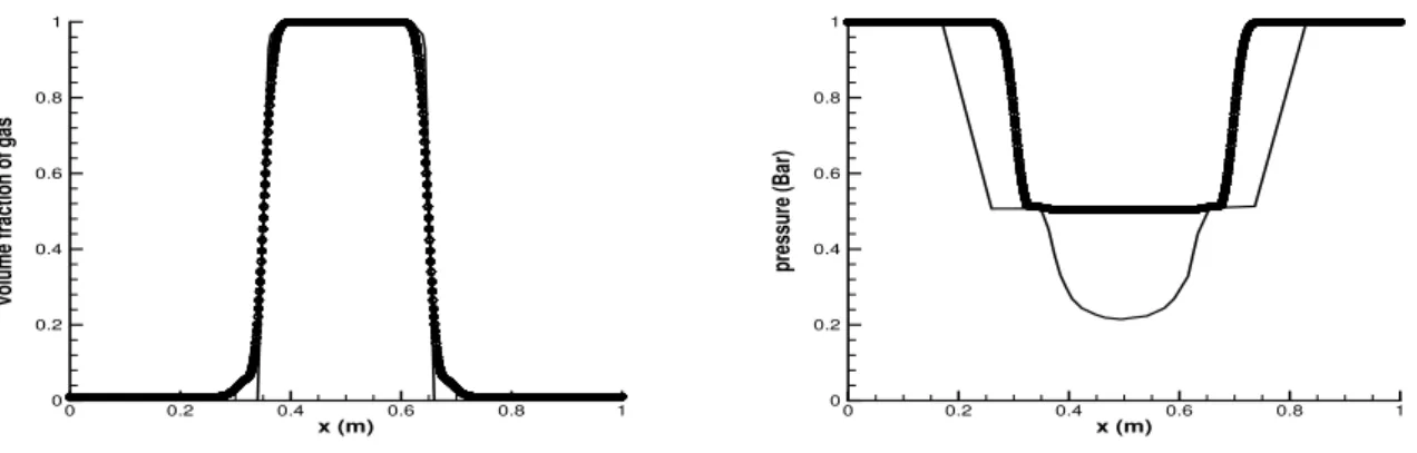
4.5 Water-air mixture expansion tube problem |u| = 2 m/s. Void fraction and pressure profiles by central scheme with 3-equation model (symbols) and 7-equation model (solid line). . . 52
4.6 Water-air mixture expansion tube problem |u| = 100 m/s. Void fraction and pressure profiles by central scheme with 3-equation model (symbols) and 7-equation model (solid line). . . 53
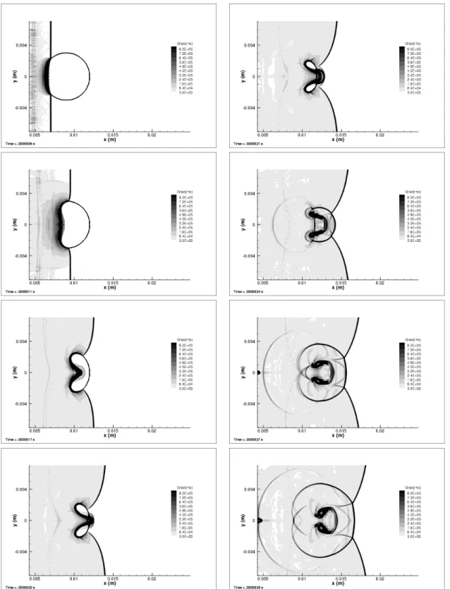
4.7 Initial situation for the shock bubble interaction D0= 0.006 m and Msh= 1.72. . . 54
4.8 Water-air shock bubble interaction. Time evolution of the density gradient. . . 56
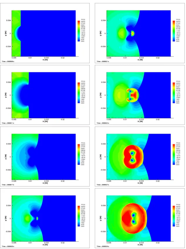
4.9 Water-air shock bubble interaction. Time evolution of the pressure (in bar). . . 57
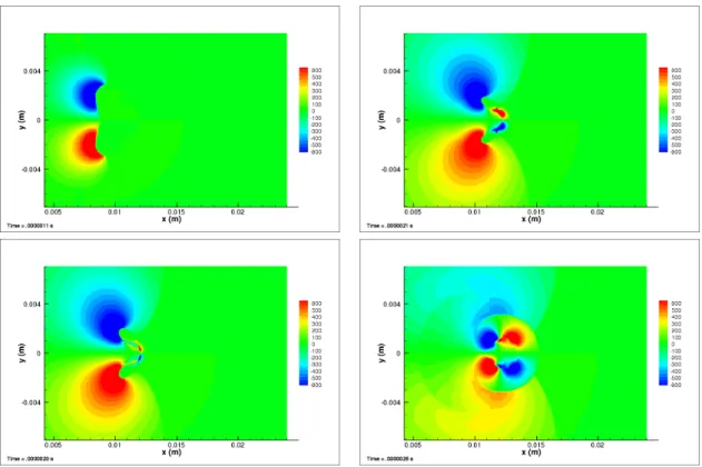
4.10 Water-air shock bubble interaction. Time evolution of the axial velocity (in m/s). . . 58
4.11 Water-air shock bubble interaction. Time evolution of the vertical velocity (in m/s). . . 58
5.1 Schematic view of the Venturi profile. . . 62
5.2 Photograph of the cavity. . . 62
5.4 Visulization of the cavity — time-averaged void ratio. . . 65 5.5 Time-averaged void ratio (left) and velocity (right) profiles from station 1 to 5 - Kunz model
comparison . . . 68 5.6 Dimensionless time-averaged wall pressure evolution - Kunz model comparison. . . . 69 5.7 RMS wall pressure fluctuations - Kunz model comparison. . . 69 5.8 µt/µ profiles from station 1 to 3 (left) and 4 to 5 (right) - Kunz model comparison . . . 70
5.9 Time-averaged void ratio (left) and velocity (right) profiles from station 1 to 5 - Merkle model comparison . . . 73 5.10 Dimensionless time-averaged wall pressure evolution - Merkle model comparison. . . 74 5.11 RMS wall pressure fluctuations - Merkle model comparison. . . 74 5.12 µt/µ profiles from station 1 to 3 (left) and 4 to 5 (right) - Merkle model comparison . . . 75
5.13 Time-averaged void ratio (left) and velocity (right) profiles from station 1 to 5 - SchnerrSauer model comparison . . . 78 5.14 Dimensionless time-averaged wall pressure evolution - SchnerrSauer model comparison. 79 5.15 RMS wall pressure fluctuations - SchnerrSauer model comparison. . . 79 5.16 µt/µ profiles from station 1 to 3 (left) and 4 to 5 (right) - SchnerrSauer model comparison. . . 80
5.17 Time-averaged void ratio (left) and velocity (right) profiles from station 1 to 5 - k − ε model with the Reboud correction comparison . . . 82 5.18 Dimensionless time-averaged wall pressure evolution - k −εmodel with the Reboud
correction comparison. . . 83 5.19 RMS wall pressure fluctuations - k −εmodel with the Reboud correction comparison. 83 5.20 µt/µ profiles from station 1 to 3 (left) and 4 to 5 (right) - k−ε model with the Reboud correction
comparison . . . 84 5.21 Time-averaged void ratio (left) and velocity (right) profiles from station 1 to 5 - k − ω SST
model with the Reboud correction comparison. . . 86 5.22 Dimensionless time-averaged wall pressure evolution - k −ωSST model with the
Reboud correction comparison. . . 87 5.23 RMS wall pressure fluctuations - k−ωSST model with the Reboud correction comparison. 87 5.24 µt/µ profiles from station 1 to 3 (left) and 4 to 5 (right) - k − ω SST model with the Reboud
correction comparison . . . 88 5.25 Time-averaged void ratio (left) and velocity (right) profiles from station 1 to 5 -
Spalart-Allmaras model with the Reboud correction comparison . . . 90 5.26 Dimensionless time-averaged wall pressure evolution - Spalart-Allmaras model with
the Reboud correction comparison. . . 91 5.27 RMS wall pressure fluctuations - Spalart-Allmaras model with the Reboud correction
comparison. . . 91 5.28 µt/µ profiles from station 1 to 3 (left) and 4 to 5 (right) - Spalart-Allmaras model with the
5.29 View of the 3D mesh composed of 251 nodes in the flow direction and 81 nodes in each transversal direction. . . 93 5.30 Time-averaged void ratio (left) and velocity (right) profiles from station 1 to 5 - Kunz model
comparison . . . 95 5.31 Dimensionless time-averaged wall pressure evolution - Kunz model comparison. . . . 96 5.32 RMS wall pressure fluctuations - Kunz model comparison. . . 96 5.33 µt/µ profiles from station 1 to 3 (left) and 4 to 5 (right) - Kunz model comparison . . . 97
B.1 (a) An isometric view of the BSCW (b) Cross-sectional view of the SC(2)-0414 airfoil (c) BSCW model mounted in TDT . . . 109 B.2 Case 1 (Mach 0.7, R e = 1.12 × 10⁷, AoA = 3°): Mean C
pfor unforced system data at 60% and
95% wing span with the SA QCR 2013 turbulence model. . . 113 B.3 Case 1 (Mach 0.7, R e = 1.12 × 10⁷, AoA = 3°): Mean Cpfor unforced system data at 60% and
95% wing span with the k − ε turbulence model. . . . 114 B.4 Case 1 (Mach 0.7, R e = 1.12 × 10⁷, AoA = 3°): Mean Cpfor unforced system data at 60% and
95% wing span with the k − ω SST turbulence model. . . . 115 B.5 Case 1 (Mach 0.7, R e = 1.12 × 10⁷, AoA = 3°): Mean Cpfor unforced system data at 60% and
95% wing span with the coarse grid. . . 116 B.6 Case 1 (Mach 0.7, R e = 1.12 × 10⁷, AoA = 3°): Mean Cpfor unforced system data at 60% and
95% wing span with the medium grid. . . 117 B.7 Case 1 (Mach 0.7, R e = 1.12 × 10⁷, AoA = 3°): Mean Cpfor unforced system data at 60% and
95% wing span with the fine grid. . . 118 B.8 Case 1 (Mach 0.7, forced oscillation at 10 Hz, R e = 1.12 × 10⁷, AoA = 3°): Mean Cp and
frequency response function of pressure due to pitch angle, 60% wing span for comparison of the turbulence models. . . 119 B.9 Case 2 (Mach 0.74, R e = 1.09 × 10⁷, AoA = 0°): Mean Cpfor unforced system data at 60% and
95% wing span with the SA QCR 2013 turbulence model. . . 121 B.10 Case 2 (Mach 0.74, R e = 1.09 × 10⁷, AoA = 0°): Mean Cpfor unforced system data at 60% and
95% wing span with the k − ε turbulence model. . . . 122 B.11 Case 2 (Mach 0.74, R e = 1.09 × 10⁷, AoA = 0°): Mean Cpfor unforced system data at 60% and
95% wing span with the k − ω SST turbulence model. . . . 123 B.12 Case 2 (Mach 0.74, R e = 1.09 × 10⁷, AoA = 0°): Mean Cpfor unforced system data at 60% and
95% wing span with the coarse grid. . . 124 B.13 Case 2 (Mach 0.74, R e = 1.09 × 10⁷, AoA = 0°): Mean Cpfor unforced system data at 60% and
95% wing span with the medium grid. . . 125 B.14 Case 2 (Mach 0.74, R e = 1.09 × 10⁷, AoA = 0°): Mean Cpfor unforced system data at 60% and
95% wing span with the fine grid. . . 126 B.15 Case 3a (Mach 0.85, R e = 1.1 × 10⁷, AoA = 5°): Mean Cpfor unforced system data at 60% and
B.16 Case 3a (Mach 0.85, R e = 1.1 × 10⁷, AoA = 5°): Mean Cpfor unforced system data at 60% and
95% wing span with the k − ω SST turbulence model. . . . 129 B.17 Case 3a (Mach 0.85, R e = 1.1 × 10⁷, AoA = 5°): Mean Cpfor unforced system data at 60% and
95% wing span with the coarse grid. . . 130 B.18 Case 3a (Mach 0.85, R e = 1.1 × 10⁷, AoA = 5°): Mean Cpfor unforced system data at 60% and
95% wing span with the medium grid. . . 131 B.19 Case 3a (Mach 0.85, R e = 1.1 × 10⁷, AoA = 5°): Mean Cpfor unforced system data at 60% and
95% wing span with the fine grid. . . 132 B.20 Case 3b (Mach 0.85, forced oscillation at 10 Hz, R e = 1.1 × 10⁷, AoA = 5°): Mean Cp and
frequency response function of pressure due to pitch angle, 60% wing span for comparison of the turbulence models. . . 133
C
H A P1
I
NTRODUCTION1.1
Background of cavitation
C
avitation is a phenomenon that occurs frequently in conventional hydraulic components such as pumps, valves, turbines and propellers. Over-speeds imposed by the local ge-ometry, shear phenomena, acceleration or vibration may cause local pressure drops in the fluid. When the flow pressure is less than the vapor pressure of the fluid, there is a partial vaporization and vapor structures arise. The so formed structures are entrained by the flow and when they reach a higher pressure zone they condense and implode violently. Cavitation leads to significant loss of system performance, problems of instability of operation of machines and erosion of the component walls. It is thus a primary source of technical problems in the field of hydraulic turbomachinery, naval propulsion and space as well as in high pressure fuel injection. However, it should be noticed that in certain cases cavitation has a desired effect, for example, supercavitation for underwater vehicles such as torpedoes. The gaseous cavities enveloping the external body make it possible to reduce the friction drag. In addition, cavitation is used for the purpose of cleaning by the control of erosion.The mechanisms of the process of cavitation and boiling are similar except that in boiling, the vaporization occurs with only small pressure change. In contrast to boiling, the vaporization in cavitation occurs under only a minor temperature change (Figure 1.1).
In the development of a space launcher, cavitation is one of the most limiting factor generated by the hydraulic because it requires from the design phase the introduction of safety margins resulting primarily from an increase in pressure in the reservoirs. This increase in pressure requires an increase in the wall thickness which generates an increase in the structure. The magnitude of this increase in dry weight is 100 k g for 100 mbar of additional pressure, which
Figure 1.1: Phase diagram of water.
corresponds about to 2% of the total weight of the largest telecommunications satellite built. Cavitation appears in the ergol turbo pumps of the launcher propellant and it generates falls of performances, instability of operation as well as mechanical loads on structures. The consequences can be tragic as the failure of the Japanese H-II launch vehicle in 1999.
As for the shipbuilding industry, cavitation is one of the major constraints in the design of marine propellers. Noise, vibration, erosion as issues resulting of cavitation are very tricky. The appearance and disappearance of bubbles on the propeller blades create local pressure fluctuations that can be compared to shock waves because of their violence. Moreover propeller produces a rotating flow in its wake. Sections of rudders that are placed behind the propeller are then in incidence and can cavitate violently at high speed. Cavitation is also very energetic and very noisy in the audible range. Depending on the type of cavitation frequencies and very specific signatures appear. This type of nuisance is obviously crucial for military vessels, as brought up to 100 km offshore by poorly controlled cavitation. The determination of cavitation instabilities regime is essential.
In the hydraulic energy field, cavitation is a limiting phenomenon in the design phase of hydraulic machinery (pumps, turbines) and its consequences in terms of erosion of the walls are a very important nuisance (operating range and duration component life). Damage to solid walls (Figure 1.2) is caused by very short pressure spikes (10ns to 1µs), high amplitude (∼ 1GPa), attributed to the impact of pressure waves emitted during the collapse of vapor structures. Knowledge of the dynamics of pockets is therefore very important. Also operating machinery instabilities related to the hydrodynamic coupling between the inter-blade channels are observed.
Figure 1.2: Damage of vane by cavitation.
1.2
Types of cavitation
There exists different patterns of cavitation according to the flow configuration, the properties of the fluid and the geometries. Generally, there are four basic types of cavitation and are described briefly below:
• Traveling cavitation
These bubbles are formed in the zone of low pressure, travel with the flow and implode after when they enter the region of higher pressure. This kind of cavitation is observed particularly in the blades of turbine or propeller (Figure 1.3).
Figure 1.3: Traveling cavitation.
• Sheet cavitation
This type of cavitation appears on the low-pressure region of blades and foils. It is a fixed, attached cavity or pocket cavitation and the fluid dynamic is largely affected by the re-entrant jet (Figure 1.4).
Figure 1.4: Sheet cavitation.
• Cloud cavitation
"Cloudy-looking" of cavitation bubbels are formed, separated and collapsed periodically by the shedding of vorticity into the flow field. It can result in intenser noise, vibration and erosion (Figure 1.5).
Figure 1.5: Cloud cavitation.
• Tip-vortex cavitation
At the tips of the rotating blade or wing, the pressure may be very low locally which will generate a filament-looking cavitation (Figure 1.6).
Figure 1.6: Vortex cavitation.
1.3
Cavitation inception
It is conventional to distinguish whether the flow is cavitating or not by means of cavitation number,σ∞, which is defined as
σ∞=
P∞− Pva p
0.5ρ∞U2 ∞
(1.1) This parameter relates the vapor pressure, Pva p, to the free-stream pressure, P∞, and the free-stream dynamic pressure.
Once the cavitation number,σ∞, is reduced in the flow, cavitation will first be observed to appear at some particular value which can be called the incipient cavitation,σi.
The pressure coefficient, CP, is given by the relation:
CP= P − P∞ 0.5ρ∞U2
∞
(1.2)
Therefore, cavitation number can be compared to the pressure coefficient and the following estimate is considered for cavitation inception,σi
σi= −CP min=
Pmin− P∞ 0.5ρ∞U2
∞
(1.3)
where CP minis the minimum pressure coefficient.
With these definitions above, it is useful to consider that if Pmin= Pva porσ∞= −CP min, the
incipient cavitation occurs which means the limiting regime between the non-cavitating and cavitating flow. If further reduction in cavitation number which implies thatσ∞< −CP min, the developed cavitation happens with an increase in the size and number of bubbles.
1.4
Objectives and organization of this thesis
Cavitation for most engineering applications is turbulent, and the interplay between cavitation and turbulence makes the cavitation dynamics even more complicated, and thus the detail dy-namics of the phase change is not well understood. Specific issues to numerical techniques in this type of flow also persist. The objectives of this thesis are to implement several cavitation models in the NSMB solver. The emphasis is placed on the study and implement of the Homogeneous Equilibrium Models (HEM) coupled with a barotropic state law and a void ratio Transport-based Equation Model (TEM). The TEM based method for the void ratio including the source terms for vaporization and condensation in the free, open source software OpenFOAM (Open source Field Operation And Manipulation) is also presented on the Venturi geometry to capture the re-entrant jet phenomenon. For the turbulence closure, a density correction approach proposed by Reboud is imposed to several turbulence models.
Besides the introduction, which presents the background of cavitation and the objectives of the study, the thesis is organized as follows.
In Chapter 2, a literature review for the modeling of two-phase flows is investigated which presents the theory in the modeling of cavitating flow, including the different models used for the present work.
In Chapter 3, the flow solvers, the NSMB and OpenFOAM, used in this study are described, including the essential elements of the governing equations, the modeling concepts and the numerical schemes.
In Chapter 4, different test cases carried out by the NSMB solver are presented together with validations against exact solutions of the Euler equations and the models implemented in the solver.
In Chapter 5, the 2D and 3D Venturi geometry are performed by OpenFOAM with the built-in solver interPhaseChangeFoam coupled with different turbulence models. Validation and comparisons are done with experimental measurements including time-averaged void ratio and velocity profiles, RMS wall pressure fluctuations.
C
H
A
P
2
R
EVIEW OF CAVITATION MODELINGN
umerical prediction of cavitation remains a challenge for several reasons. First the mod-eling of phase transition (thermodynamics) and the interactions with the turbulence is not fully established. In addition, it is a complicated task to deal with the large variations of density between the liquid and vapor phases. Specific issues to numerical techniques in this type of flow also persist. On the issue of numerical architecture (compressible or incompressible low Mach preconditioning extended to variable densities), the question remains open. However, several studies have shown better capture re-entrant jet of cavitation bubbles by compressible codes [Venkateswaran et al., 2002; Goncalvès et al., 2010a; Park et al., 2012; Skoda et al., 2012].2.1
Modeling of two-phase flows
In this chapter only the modeling of gas-liquid flows are presented. There exists two main approaches for the gas-liquid flows :
• Direct or interface-based methods
• The averaged or diffusion methods of the interface
2.1.1 Direct resolution methods
The so-called direct resolution methods allow to solve all the spatial and temporal scales of the two-phase flows. These kinds of methods reconstruct the interfaces and describe the propagation of the flow, while solving the Navier-Stokes equations.
• Front tracking method (Lagrangian) • Level Set method (Eulerian)
• Volume Of Fluid method (Eulerian)
• Diffuse interface method ([Jamet et al., 2004])
Because of the existence of various velocities at the interface i.e. liquid phase velocity, vapor phase velocity and interface velocity, phase changes are difficult to be taken into account in these kinds of methods. Moreover, the reconstruction of the interface in three-dimensional flows can be difficult and very time consuming.
2.1.2 The average resolution methods
In most of these problems, it is not necessary and would be extremely difficult to know the instantaneous values of the local variables of the flow due to the limitation of the capabilities of computers and the difficulty in predicting the position of the interfaces. The prediction of "averaged" properties are mostly interested in, such as the pressure drop in a bubble flow, the volume flow rate in a conduit etc...
For this purpose, "averaged" forms of the equilibrium equations will be used to predict mean val-ues of the flow parameters which are meaningful and experimentally accessible. Moreover, since the equations of equilibrium appear in the form of partial differential equations, it is desirable that the mean properties and their first derivatives, spatial and temporal, should be continuous. The presence of interfaces leads to serious difficulties for the mathematical formulation of the problem, in the same way as the shock waves in single phase.
The concept of beginning with these methods is the use of instantaneous conservation laws of fluid mechanics for each phase. The interfaces appear as surfaces of discontinuity for the different properties of the fluid, so the fundamental equilibrium equations are expressed in the form of "averaged interface conditions".
There are many ways to "average". Averaging of conservation laws can be carried out: • in space
• in time
• statistically from a set of measures
Spatial averaging has been mainly used in the field of nuclear engineering (average over a section of a pipe). It allowed the development of 1D code for the safety analysis of nuclear reactors by averaging the equations on the section of a pipe.
Similar to the use of the RANS approach for turbulent single-phase flows, the temprol averaging is widely used for two-phase flows, especially if they are turbulent. Indeed, since transport phenomena are highly dependent on local fluctuations of variables, it is easier in this case to link the laws of state and behavior needed to close the problem with experimental measurements [Ishii and Hibiki, 2011] .
2.1.3 Local time-averaged equations
In single-phase turbulent regime, an approach in the sense of Reynolds averaged which treats the instantaneous Navier-Stokes equations statistically is used. For a steady flow, the overall average of equations (average obtained over a large number of realizations) can be replaced by a temporal averaging (ergodic hypothesis).
In the two-phase flow; the location of the interface is unknown in time and space, the instanta-neous equations can not be solved. The equations are averaged by decomposing each variable into an average part and a fluctuating part.
The temporal averaging operator of the instantaneous equations reveals the presence rateα, defined by:
α=Tk
T (2.1)
which represents the time Tkof the presence of the phase k, with respect to a duration T. After spatial discretization of the computational domain, the presence rate is averaged over each cell and is then expressed as the volume fraction:
α=
Vk
V (2.2)
where Vk is the volume of the phase k in a volume mesh V .
2.1.4 The different models
Different classes of models are present in the literature according to the number of conserva-tion laws treated and the assumpconserva-tions made: equilibrium model/relaxed model, homogeneous model/two-velocity model, two-fluid model/one-fluid model:
• Two-fluid models
The full seven-equation two-phase models proposed by Baer et Nunziato [Baer and Nun-ziato, 1986] are the most complete. These models take into account explicitly the non-equilibrium effects between phases (unnon-equilibrium of pressure, velocity and temperature)
but remain difficult to be used in industrial flows (turbomachinery). A seven-equation model has been used for supercavitation and expansion tube problems by Saurel [Métayer et al., 2005; Saurel and Metayer, 2001]. The two-fluid method remains more suited for inviscid and simple geometries [Métayer et al., 2005; Saurel et al., 2008a; Petitpas et al., 2009; Zein et al., 2010; Saurel and Metayer, 2001; Yeom and Chang, 2006, 2013].
• One-fluid homogeneous mixture models
The models are composed of three conservation laws written for the mixture and are based on a assumption of non-slip between the phases. With the assumption of thermo-dynamic equilibrium, the Homogeneous Equilibrium Models (HEM) are constituted. The non-equilibrium effects can be introduced empirically [Yoon et al., 2006]. Different equa-tions of state for the mixture have been developed in cavitation in a thermosensitive fluid : barotropic law [Cooper, 1967; Rapposelli and d’Agostino, 2003], algorithm for calculating temperature based on the equality of the free enthalpies between the phases [Edwards and Franklin, 2000].
• Reduced models with five equations
These models are obtained from a simplification of the complete two-fluid model. The archetype five-equation model is the one of Kapila [Kapila et al., 2001] which is composed of two conservation equations for masses, one conservation equation for the mixture momentum, one conservation equation for the mixture energy and one non-conservative equation for the void ration to describe the flow topology. They involve two temperature which makes it possible to reproduce thermal non-equilibrium effects, as proposed in the model of Saurel [Saurel et al., 2008b] for cavitation simulation in diesel injectors. Some formulations have been proposed to the simulation of interface between two fluids [Allaire et al., 2002; Kreeft and Koren, 2010; Murrone and Guillard, 2005; Tian et al., 2011]. • Relaxed models with four equations
A four-equation model was developed for a flashing flows and ebullition applications : the Homogeneous Relaxation Model (HRM). It consists of three conservation laws for the mixture and one additional transport equation for the void ratio. The latter contains a relaxation source term. The source term involves a relation time that is the time for the system to regain its thermodynamic equilibrium state. This relaxation time is very difficult to determine and is estimated from experimental data [Barret et al., 2002; Downar-Zapolski et al., 1996]. Another formulation of the relaxation term was proposed by Helluy [Helluy and Seguin, 2006], based on a constrained convex optimization problem on the mixture entropy.
Another four-equation model which is very popular to simulate cavitating flows in cold water has been adapted to cryogenic application [Hosangadi and Ahuja, 2005; Utturkar et al., 2005; Zhang et al., 2008] by adding a transport equation for the void ratio : the
Transport-based Equation Model (TEM). This equation includs a cavitation source term for the modeling of condensation and vaporization. The main difficulty is related to the formulation of the source term and the tunable parameters involved for the vaporization and condensation process. The calculation of the void fraction by an additional transport equation including the source terms for vaporization and condensation processes is increas-ingly used for this model. In this case, the term of mass transfer between phases must be treated explicitly. Several empirical formulations have been proposed to simulate cavitating flows [Ahuja et al., 2001; Wang and Ostoja-Starzewski, 2007; Merkle et al., 1998; Singhal et al., 2002; Venkateswaran et al., 2002; Vortmann et al., 2003; Wu et al., 2005; Morgut et al., 2011; Kunz et al., 2000; Senocak and Shyy, 2002; Hosangadi and Ahuja, 2005] but still suffer from a calibration problem and thermodynamics inconsistency [Goncalvès and Patella, 2011]. Different sets of parameters are presented in [Utturkar et al., 2005; Frikha et al., 2008; Agnieszka et al., 2016].
The different classes of models are summarized in Table 2.1.
Models Seven equations Five equations Four equations Three equations
Equations 2 mass 2 mass 1 mass 1 mass
2 momentum 1 momentum 1 momentum 1 momentum 2 energy 1 energy 1 energy 1 energy
+α +α +α
Characteristic 2 pressure 1 pressure 1 pressure 1 pressure 2 velocity 1 velocity 1 velocity 1 velocity 2 temperature 2 temperature 1 temperature 1 temperature Appellation two-fluid reduced one-fluid relaxed one-fluid
HRM or TEM HEM ou HNEM Applications 1D Euler 2D Euler 2D, 3D N-S 2D, 3D N-S
Table 2.1: Class of models for cavitating flows
2.1.4.1 The two-fluid model
This model is about the Navier-Stokes equations for those phases involved. Here the case of two phases is considered, where k is the phase index, k=1, 2. This gives the following six conservation equations : ∂αkρk ∂t + ∇. ¡ αkρkuk ¢ = Γk (2.3) ∂αkρkuk ∂t + ∇. ¡ αkρkuk⊗ uk¢ = −∇(αkpk) + ∇.(αkτk) +αkρkFk+ Mk (2.4) ∂αkρkEk ∂t + ∇. ¡ αkρkEkuk¢ = −∇.£αkqk¤ − ∇.£puk¤ + ∇. h τk.uk i +αkρkFk.uk+ Qk (2.5)
E = e +12u2is the specific total energy.
Γk, Mk, Qk are the source terms relating to transfers of mass, momentum and energy between
phases. They represent the interfacial effects and must be modeled.
Mk= MΓk+ PkI∇αk+ Fkd (2.6) The term MΓk represents the momentum transfer due to the mass transfer. Fkdcorresponds to the interfical friction force exerted on the phase k. PkIis the pressure of phase k at the interface.
Qk= HkΓ− pkI∂αk
∂t + F
d
k.ukI+ QkI (2.7)
HΓk= Lva pΓk represents the energy transfer due to the mass transfer, where Lva pis the latent
heat of phase change. QkI corresponds to the interfacial heat transfer. ukIis the vector of velocity of phase k at the interface.
In addition: 2 X k=1 Mk= Mm= 0 and 2 X k=1 Qk= Qm= 0 (2.8) It should notice that these two terms are not necessary equal to zero although they are generally be taken like that. Indeed due to the variation of the curvature of the interface, the momentum and the energy provided by one phase are not equal to those received by the other.
2.1.4.2 The one-fluid model
This model, also known as homogeneous mixture approach of two-phase flow consists in writing the averaged Navier-Stokes equations for a "mixing" fluid. It is assumed that the two phases move at the same velocity (i.e. neglecting the drag term between phases). The exchanges and the unequilibrium between phases are then no longer directly modeled, but it is possible to represent them in the closure of the system. Actually, the equation of state of the mixture may introduce a difference at the saturation point (for example, the barotropic law).
A physical property of the mixture is defined by a weighting of the void ratio to its value between each phase. For the weighting of the extensive properties, the density will be used.
ρm =αρV+ (1 −α)ρL and ρmem =αρVeV+ (1 −α)ρLeL (2.9)
The conservation equations are as follows :
∂ρm ∂t + ∇. ¡ ρmum ¢ = 0 (2.10) ∂ρmum ∂t + ∇. ¡ ρmum⊗ um ¢ = −∇(pm) + ∇.(τm) +ρmFm (2.11) ∂ρmEm ∂t + ∇. ¡ ρmEmum ¢ = −∇.£ qm¤ − ∇.£pum¤ + ∇. h τm.um i +ρmFm.um (2.12)
It can be observed that the energy required for phase change, the latent heat, does not appear explicitly in the energy conservation equation. In fact, this term is treated implicitely for the mixture.
2.1.4.3 Four-equation models
These models are intermediate models between one-fluid and two-fluids ones. It consists of solving the conservation equations for the mixture plus a continuity equation for one phase. This makes it possible to treat the mass transfer term explicitly.
∂ρm ∂t + ∇. ¡ ρmum ¢ = 0 (2.13) ∂ρmum ∂t + ∇. ¡ ρmum⊗ um ¢ = −∇(pm) + ∇.(τm) +ρmFm (2.14) ∂ρmEm ∂t + ∇. ¡ ρmEmum ¢ = −∇.£ qm¤ − ∇.£pum¤ + ∇. h τm.um i +ρmFm.um (2.15) ∂α1ρ1 ∂t + ∇. ¡ α1ρ1u1 ¢ = Γ1 (2.16)
There exists different models according to the modeling of the mass exchange term between the phases.
2.1.5 The equations of state
From the thermodynamic point of view, two state variables are sufficient to represent the thermodynamic state of a fluid. The main relationships existing in the literature are :
• Incompressible fluid • Tait law
• Perfect gas law • Van der Waals law • Mie-Grüneisen type law • Stiffened gas law • Tammann law
2.1.5.1 Incompressible fluid
This assumption leads to a very simplified state law :ρ=ρ0
and Cp = Cv = C which are the specific heats at constant pressure and constant volume res-pectively. This equality leads to the following relation between the internal energy and the
temperature : d e = CdT
This assumption has the effect of decoupling the mass conservation equation and the momen-tum conservation equation with the energy conservation equation. In fact, the temperature no longer appears in the first two equations,therefore it has no more influence on the other physical properties.
2.1.5.2 Tait law
For the case of a slightly compressible flow it is possible to take into account the compressibility of a fluid by the relation :∆P = c2∆ρ
Tait law : ρ
ρre f =
p
[ n] P + P0
Pre f+ P0 whereρre f and Pre f are reference density and pressure. For water, P0= 3 × 10⁸and n = 7.
It is the formulation used by [Venkateswaran et al., 2002; Pouffary, 2004] to take into account the compressibility in the pure phases for the modeling of cavitation. The speed of sound c is a given value for each phases.
2.1.5.3 Perfect gas law
This state law allows to model a large number of gases with a good approximation: PV = nRT avec R=8.314 J/(K.kg).
It is also written in the form: P =ρrT where r = R/M = Cp− Cv(=287 SI unit for air).
According to the internal energy : P¡
ρ, e¢ = (γ− 1)ρe whereγ=Cp
Cv is the ratio of specific heats.
With Joule’s law :∆e = Cv∆T and ∆h = Cp∆T where Cvand Cpare constants.
There is also the semi-perfect gas law, which defines Cp(T) and Cv(T) no longer to be constant, but by using polynomial laws as a function of temperature.
2.1.5.4 Van der Waals law
This law was first introduced by van der Waals in 1873. It contains two constants a and b which are calibrated on the behavior of the fluid at the critical point. It represents one of the first state laws for real gases.
µ P + a
v2
(v − b) = rT where v is the specific volume (2.17) This law produces a negative sound speed (dP/dρ< 0) in the phase transition zone (unstable thermodynamic equilibrium).
2.1.5.5 Stiffened gas law
This low is detailed in [Rolland, 2003]. It is valid for a large number of fluids, and is sometimes used for solids : P¡
ρ, e¢ = (γ− 1)ρ(e − q) −γp∞
The term (γ−1)ρ(e − q) represents the intermolecular repulsive effect. The term −γp∞represents the molecular attraction which is responsible for the cohesion of liquids or solids. This term is null for the perfect gas state law.
It is set for each fluid by the constantsγand p∞(q=0). In the phase change the parameter q, which refers to the energy of the fluid at a given reference state, is non-zero.
The heat capacities are constants in the approximation of stiffened gas law. In the same way as for the perfect gas law, a semi-stiffened gas law makes it possible to define Cv and Cp by polynomial laws as a function of temperature.
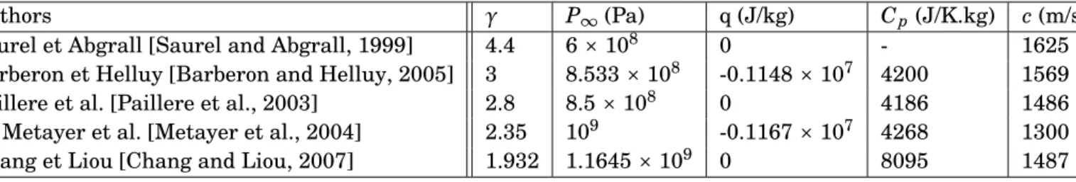
Several sets of parameters for cold water have been proposed as shown in Table 2.2 :
Authors γ P∞(Pa) q (J/kg) Cp(J/K.kg) c (m/s)
Saurel et Abgrall [Saurel and Abgrall, 1999] 4.4 6 × 10⁸ 0 - 1625 Barberon et Helluy [Barberon and Helluy, 2005] 3 8.533 × 10⁸ -0.1148 × 10⁷ 4200 1569 Paillere et al. [Paillere et al., 2003] 2.8 8.5 × 10⁸ 0 4186 1486 Le Metayer et al. [Metayer et al., 2004] 2.35 109 -0.1167 × 10⁷ 4268 1300 Chang et Liou [Chang and Liou, 2007] 1.932 1.1645 × 10⁹ 0 8095 1487
Table 2.2: Parameters of the stiffened gas law for cold water by different authors
2.1.5.6 Tamman law
This law is equivalent to the stiffened gas law :P + Pc=ρLK (T + Tc)
The use of parameters Pc, K , Tc, is another formulation but is equivalent to those of stiffened
gas law q, P∞andγ.
2.1.5.7 Mie-Grüneisen type law
This law is written as : P(ρ, e) = P∞(ρ) +Γ(ρ)ρhe − ere f(ρ)i whereΓ =1ρ ∂p∂e¯¯
¯ρ is the coefficient of Grüneisen and P∞(ρ) is given as a function of the fluid. The stiffened gas law is obtained with the assumption of low density variations from the Mie-Grüneisen law. For isentropic evolutions, it becomes the Tait law. Another particular case : if P∞ is null, then the perfect gas law is obtained.
2.1.5.8 Benedict-Webb-Rubin law
To get as close as possible to the representation of real gases, there are even more complex form of state laws such as the Redlich-Kwong-Soave equation or the Benedict-Webb-Rubin equation [Benedict et al., 1940].
The Benedict-Webb-Rubin law is written as :
P = RTd + d2¡RT (B + bd) − ¡A + ad − aαd4¢¢ − 1
T2¡C − cd ¡1 +γd 2
¢ exp¡−γd2¢¢
With P the pressure, R the perfect gas constant, T the temperature, d the molar density, and a, b, c, A, B, C,α,γthe empirical parameters. This law is for example used to represent refrigerants. It is used to characterize hydrogen in the formulation "condensable fluid" in the code FineT M/Turbo.
2.1.6 Presentation of different models of cavitation
In this section, a review of various models available in the literature that describe the phenomena of cavitation with or without the consideration of thermodynamic effect is presented.
In cold water, or more generally for a non-thermosensitive fluid, the dynamic and thermal phenomena are decoupled. The energy equation is therefore not necessary.
In contrary, in thermosensitive fluid, it is necessary to include the equation of energy.
2.1.6.1 Models with the mixture state law
These are models with three equations (or two equations without the energy) for which the phase change is controlled by a state law. There are several types of closure relations to link the two phases in the literature :
• Sinusoidal barotropic law [Delannoy and Kueny, 1990]
• Logarithmic barotropic law [Schmidt et al., 1999; Moreau et al., 2004; Xie et al., 2006] • Saurel’s equilibrium law [Saurel et al., 1999]
• Tabulated state law [Ventikos and Tzabiras, 1995; Clerc, 2000]
• Equilibrium law based on free enthalpy [Edwards and Franklin, 2000] • Polynomial law (of degree 5) [Song, 2002]
• Barotropic law "Italian" [Rapposelli and d’Agostino, 2003; Sinibaldi et al., 2006]. • State law based on entropy [Barberon and Helluy, 2005]
a/ Sinusoidal barotropic law
The barotropic model existing in FineT M/Turbo was developed by the successive theses of Coutier [Coutier-Delgosha, 2001] and Pouffary [Pouffary, 2004]. It was originally proposed by Delannoy et Kueny [Delannoy and Kueny, 1990]. This law relates the pressure to the density by a sinusoidal relation : ρ=ρL+ρV 2 + ρL−ρV 2 sin à p − pva p c2min 2 ρL−ρV ! (2.18) cminrepresents the minimum speed of sound in the mixture. This law introduces a small non-equilibrium effect on the pressure. The unnon-equilibrium is controlled by the value of cmin.
b/ Schmidt’s barotropic law
From the integration of the Wallis mixture speed of sound which is the propagation velocity of acoustic waves without mass transfer, Schmidt [Schmidt, 1997] proposes a barotropic law in the form of : P = psat+ ρVc2VρLc2L¡ ρV−ρL ¢ ρ2 Vc 2 V−ρ 2 Lc 2 L ln " ρVc2V¡ ρL+α¡ρV−ρL ¢¢ ρL¡ ρVc2V−α¡ ρVc2V−ρLc2L¢¢ # (2.19)
This expression is used in [Moreau et al., 2004; Dumont, 2004] to simulate the cavitation of diesel in the injectors of piston engine. A modified version was proposed by [Xie et al., 2006] in order to avoid the appearance of negative pressure.
c/ Saurel’s equilibrium law
For compressible flows, Saurel [Saurel et al., 1999] uses the Tait law for the liquid and the perfect gas law for the vapor to calculate the pressure in each phase. The mixture is assumed to be in kinematic and thermodynamic equilibrium. In this way, there is a logarithmic relation to connect P and T in the form of :
ln(P/P0) =
X
k
ak(T/T0)k (2.20)
The densities of each phase are given by polynomial functions of the temperature. The void ratio is defined as :
α= ρ−ρLsat(T)
ρV sat(T) −ρLsat(T)
(2.21)
d/ Edwards equilibrium law
Edwards et al. [Edwards and Franklin, 2000] propose an equilibrium model to simulate two-phase octane flows. The pure two-phases are governed by Sanchez-Lacombe’s law. Thermodynamic equilibrium is defined by the equality of free enthalpies (g = h − Ts) between phases : gL= gV.
The iterative resolution of this equation makes it possible to determine the vapor pressure Pva p(T). The void ratio is calculated by :α=ρ ρ−ρLsat(T)
e/ Rapposelli’s barotropic law
Using thermal analysis on a bubble, a relation between the speed of sound in the two-phase mixture and the temperature can be obtained [Rapposelli and d’Agostino, 2003]. It is possible to find a law between the density and the temperature by integrating the speed. This law has been used for the calculation of hydrofoil in non-viscous flow.
The speed of sound is expressed as the relation : 1 ρc2 = 1 ρ ∂ρ ∂p∼= 1 −α p " ¡1 −εL¢ p ρLc2L+εLg ∗µpc p ¶η# +γα Vp (2.22) In this expression, γV = C pCvV
V and εL represent the liquid fraction participating in the heat exchanges with the vapor and :
εL= α 1 −α " µ 1 +δT R ¶3 − 1 # (2.23) where δT
R is a controlled parameter obtained from calibration of the model from experimental
results. The other parameters are as follows :
For cold water : g∗= 1.67;η= 0.73; Pc= 221.29 105 Pa
For nitrogen : g∗= 1.3;η= 0.69; P
c = 3.4 106 Pa
f/ State law based on entropy
Barberon et Helluy [Barberon and Helluy, 2005] proposed to calculate the entropy of the mixture to evaluate the pressure and the temperature. The pure phases are both governed by the stiffened gas law. The specific entropy of the mixture is maximal at thermodynamic equilibrium. During the process of maximization the entropy can be determined when equilibrium is reached and then also for the pressure P = T∂v∂s , where v is the specific volume.
g/ Mixture of stiffened gas law
With the assumption of thermal and mechanical equilibrium, an expression for the pressure and the temperature can be deduced as follows [Goncalves and Patella, 2009] :
P¡ ρ, e,α¢ = (γ(α) − 1)ρ(e − q(α)) −γ(α)P∞(α) 1 γ(α) − 1 = α γV− 1+ 1 −α γL− 1 and ρq(α) =αρVqV+ (1 −α)ρLqL P∞(α) = γ(α) − 1 γ(α) " αγVP V ∞ γV− 1+ (1 −α )γLP L ∞ γL− 1 # T¡ ρ, h,α¢ = h − q(α) C p(α) with ρC p(α) =αρVC pV+ (1 −α)ρLC pL The void ratio is computed with saturation values of densities :α= ρ−ρLsat
An extension version considering thermodynamic effects for thermosensible fluids is proposed in [Goncalves and Patella, 2010] by introducing a linear variation relation of Pva p,ρLandρV with
the temperature.
However, this law failed to obtain reasonable results for Venturi case of 4 degree.
2.1.6.2 Models with four equation, transport-based equation models (TEM)
In these models, a conservation equation for one of the phases is added by means of the source term S which models the mass exchange between the phases. There are different formulations for the source term (more or less empirical constants) :
• Merkle’s model [Merkle et al., 1998] • Kunz’s model [Kunz et al., 2000]
• Senocak and Shyy model [Senocak and Shyy, 2002] • Saito’s model [Saito et al., 2003]
• Vortmann’s model [Vortmann et al., 2003] • Utturkar’s model [Utturkar et al., 2005]
• Hosangadi and Ahuja model [Hosangadi and Ahuja, 2005] • Goncalvès model [Goncalvès, 2013]
• Source term based on the simplified Rayleigh-Plesset equation
a/ Merkle’s model (1998)
The model proposed by Merkle [Merkle et al., 1998] is one of the first models that uses the mass conservation equation for the vapor phase to simulate the cavitation.
The equation solved for the vapor phase is as follows:
∂xV ∂t + u.∇xV= − xV τV = xL τL (2.24)
where xV and xLare the mass fractions of the vapor and liquid phases respectively (αρV = xVρ).
The source term is defined as:
1 τV = ( 0 when P < Pva p 1 kτre f ¯ ¯ ¯ P−Pva p q ¯ ¯ ¯ when P > Pva p
τLis defined in the same way for condensation.
τre f=
Lre f
Ure f is the reference time scale of the fluid, and k is a constant with the value around 10 −3.
The parameter q is not specified in the article [Merkle et al., 1998] but seems to be the reference dynamic pressure q = 0.5ρUre f2 .
b/ Kunz’s model (2000)
Kunz’s model [Kunz et al., 2000] is based on an empirical source term split into two contributions for the evaporation and condensation process :
∂αL
∂t + ∇.(αLu) =¡ ˙m
++ ˙m−¢
(2.25) This model is implemented in the IZ code [Coutier-Delgosha et al., 2002, 2003; Patella et al., 2006]. The evaporation and condensation source terms are given as following expressions :
˙ m−= Cd estρVαLM in(0, P − Pva p) ρL(ρLU2re f/2)t∞ and m˙+= CprodρVα2L(1 −αL) ρLt∞ (2.26) where t∞is the relaxation time, Cd estand Cprodare the constants to be calibrated.
The condensation rate is modeled as being proportional to the liquid volume fraction and the amount by which the pressure is below the saturated vapor pressure. For the evaporation rate, a simplified Ginzburg-Landau relationship is used.
c/ Senocak and Shyy model (2001)
Senocak et Shyy [Senocak and Shyy, 2002] try to eliminate the empirical constants by adopting from Kunz’s model. It is carried out by the idea of introducing the normal interfacial velocity. However there will be a problem of locating the interface arises. This difficulty is overcome by the calculation of the density gradient. In this way, a fictitious interface is obtained because of modeling effort inside it (see Figure 2.1). The mass transfer source terms are as follows :
˙ m−= ρVαLM in(0, P − Pva p) ρV(UV ,n−UI,n)2(ρL−ρV)t∞ and m˙+= (1 −αL)Max(0, P − Pva p) (UV ,n−UI,n)2(ρL−ρV)t∞ (2.27)
where UV ,n= u.n with n =|∇α∇αL L|
The normal interfacial velocity, UI,n, is zero in steady calculation. This model is called Sharp
Interfacial Dynamics Model (IDM).
d/ Saito’s model (2003)
Saito [Saito et al., 2003] uses a mass transfer equation for the vapor phase. The system is closed by the modeling of the source term and a mixture state law. The mixture state law is determined by the weighting of each phase form the Tamman law for the liquid phase and the perfect gas law for the vapor phase respectively. :
1 ρ = 1 ρL(1 − x) + 1 ρV x or ρ= P¡P + Pc ¢ K (1 − x) P(T + Tc) + rx¡P + Pc¢ T (2.28) The vapor pressure is given by an empirical formula as a function of the temperature. The mass transfer source term is proportional to the pressure difference, Pva p− P, as well as the inverse of
the square root of the saturation temperature.
˙ m = ˙ m+= CeAα(1 −α)ρL ρV P∗ V a p− P p2πRTS if P < Pva p∗ ˙ m−= CcAα(1 −α) P∗ va p− P p2πRTS if P ≥ Pva p∗
where TSis the saturation temperature and A = Caα(1 −α)
A denotes the interfacial area concentration in the vapor-liquid mixture.
The saturation vapor pressure of cold water is given by the empirical formula as : Pva p∗ = 22.13 × 10⁶exp ½µ 1 −647.31 T ¶ ¡7.21379 + ¡1.152 × 10⁻⁵− 4.787 × 10⁻⁹T¢ (T − 483.16)2¢ ¾
The parameters Ca, Ccand Ce are empirical constants.
e/ Vortmann’s model (2003)
A rate equation for vapor quality x is formulated by Vortmann [Vortmann et al., 2003] as :
∂x
∂t + u.∇x = (1 − x)Kl→v− xKv→l (2.29) The terms Kl→v and Kv→l mean the probabilities of phase change from liquid to vapor and from vapor to liquid respectively. These terms integrate the Gibbs free energy and involve the relaxation time set to 10−4s kg/m3. The vapor pressure is supposed to be constant.
f/ Utturkar’s model (2005)
The previous IDM model is adapted by Utturkar et al. [Utturkar et al., 2005] to take the thermodynamic effects into account. The new model is then called Mushy Interfacial Dynamics Model. The original model without thermodynamic effects uses the averaged interface coditions of a liquid-vapor interface to construct the mass transfer source term. This approach is justified by the authors that the sheet cavitation of the cold water contain a significant void ratio. Starting from the analysis of Hord [Hord, 1974] for the composition of cryogenic sheet cavitation which describes the vapor zone as the mixture zone with lower void ratio, a model using the averaged