HAL Id: hal-02435796
https://hal.archives-ouvertes.fr/hal-02435796
Submitted on 13 Jan 2020
HAL is a multi-disciplinary open access
archive for the deposit and dissemination of
sci-entific research documents, whether they are
pub-lished or not. The documents may come from
L’archive ouverte pluridisciplinaire HAL, est
destinée au dépôt et à la diffusion de documents
scientifiques de niveau recherche, publiés ou non,
émanant des établissements d’enseignement et de
Distinguishing and Classifying from n-ary Properties
Pascal Préa, Monique Rolbert
To cite this version:
Pascal Préa, Monique Rolbert. Distinguishing and Classifying from n-ary Properties. Journal of
Classification, Springer Verlag, 2014, 31 (1), pp.28-48. �10.1007/s00357-014-9151-1�. �hal-02435796�
Distinguishing and Classifying from n-ary
Properties
Pascal Pr´ea
´
Ecole Centrale Marseille,
Laboratoire d’Informatique Fondamentale de Marseille,
LIF, CNRS UMR 7279,
Technopˆole de Chˆateau-Gombert, 38, rue Joliot-Curie,
13451 Marseille Cedex 20, France
Monique Rolbert
Aix-Marseille Universit´e,
Laboratoire d’Informatique Fondamentale de Marseille,
LIF, CNRS UMR 7279,
Marseille, France
{prea,rolbert}@lif.univ-mrs.fr
Abstract
We present a hierarchical classification based on n-ary relations of the enti-ties. Starting from the finest partition that can be obtained from the attributes, we distinguish between entities having the same attributes by using relations between entities. The classification that we get is thus a refinement of this finest partition. It can be computed in O(n + m2) space and O(n · p · m5/2) time, where n is the
number of entities, p the number of classes of the resulting hierarchy (p is the size of the output; p < 2n) and m the maximum number of relations an entity can have (usually, m n). So we can treat sets with millions of entities.
Keywords: Classification, Data Analysis, Hierarchy, Ultrametric, Computa-tional Linguistics, Generation of Referring Expressions.
1
Introduction
Many algorithms and methods in classification and data analysis are based on the at-tributes of the entities (see Barth´elemy and Gu´enoche 1991; Gordon 1999; Jardine and Sibson 1971).For instance, classical taxonomy (see Buffon 1749; Linn´e 1735) classi-fies living species according to some attributes, such as having hair, feathers, or scales. Ecology, i.e. relations between animals (like who eats who or who parasitizes who) or between an animal and its surroundings, is a meta-knowledge which is not taken into account by taxonomy. Since it seems that we are living a mass extinction event,
and although such an event is measured by the number of disappearing taxa, ecology is becoming more and more important. When an animal disappears, the impact of its extinction is more related to its ecological role than to its place in the evolution tree (the quasi-extinction of tigers does not affect lions, although tigers and lions are very close species, but the extinction of gnus would have heavy consequences for lions). Another example of the importance of links and relations between entities is that, with the growing influence of social networks, it is often said that the identity of a person is more who, and how, he is linked to than his own qualities.
In this paper, we present a hierarchical classification of entities using not only at-tributes but also relations between the entities. Actually, this idea comes from previous work (see Rolbert and Pr´ea 2009) in computational linguistics: we tailor a solution to a classical problem in computational linguistics (the generation of referring expressions) and show that this solution yields an efficient method for classifying objects.
We first present the general purpose of generating referring expressions. Then, in section 3, we give a precise definition of distinguishability (i.e. we give necessary and sufficient conditions for an entity to admit a referring expression) that takes into account n-ary relations between entities. We show that this definition yields a hier-archical classification of the entities. In section 4, we give an O(n + m2) space and O(n · p · m5/2) time algorithm to compute this hierarchy, where n is the number of entities, p the number of classes of the resulting hierarchy (p is the size of the out-put; p < 2n) and m the maximum number of relations an entity can have (usually, m n). This algorithm is efficient enough to treat data sets with millions of entities. In the penultimate section, we will apply our method to classical attribute data, namely the Fisher iris data (from Fisher 1936). In the last section, we will mention some related work and possible extensions.
2
The generation of referring expressions
The generation of referring expressions has been a classical task in natural language processing for more than twenty years. Its aim is to generate a definite description (the referring expression) which designates one and only one entity among others in a context set like a scene or a discourse (see Dale 1989; Deemter 2002; Krahmer et al. 2003; Croitoru and Deemter 2007). An entity which admits such a description is said to be distinguishable.
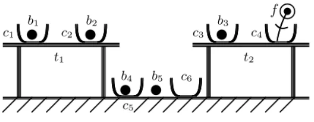
Let us see this more precisely in the example in Figure 1.
In this scene, the entities are tables (t1 and t2), cups (c1. . . c6), balls (b1. . . b5), a flower (f ) and the floor. For the sake of simplicity, let us suppose that this scene is described using unary relations (like is a table or is a flower), and only two binary relations: being in/containing, being on/having on. So, we have:
t1is a table which has c1and c2on it. c1is a cup which is on t1and contains b1 b2is a ball which is in c2
t1 t2 c1 c2 c3 c4 c5 c6 v b1 v b2 v b3 v b4 v b5 ti f
Figure 1: A simple scene
b5is a ball which is on the floor. . . .
From this description, one can designate these entities by using the following referring expressions:
f : The flower
b5: The ball on the floor c4: The cup with a flower in it
c5: The cup on the floor with a ball in it c6: The empty cup
b3: The ball in a cup which is on a table on which there is a cup containing a flower . . .
The aim of the generation of referring expressions is to make a computer do the same thing, and more precisely to produce an expression close to what would be produced by a human being. Following this goal, most works in generation of referring expressions do not focus on formal determination of what is a distinguishable entity, especially when this distinguishability does not have a “natural expression” (see Gardent 2002; Khan et al. 2009; Mitchell 2009). For instance, the entity b3may be considered as non-distinguishable, since its referring expression is rather long (a human being would not use it). Other works (see Khramer et al. 2003; Deemter and Krahmer 2006; Rolbert and Pr´ea 2009) tend to explore, in a systematic and complete way, all the relations which can yield distinguishability. We will apply this approach to classification.
3
An iterative definition for distinguishability and a
hi-erarchical classification of entities
Intuitively, an entity e1is distinguishable from an entity e2in two cases:
• e1 and e2 do not have the same set of properties (we will say that e1 is 0-distinguishablefrom e2). In the example of Figure 1, the entity b3is 0-distinguishable from f since b3has a property (is a ball) that f does not have. More generally, in the example of Figure 2, the tables t1 and t2 are 0-distinguishable one from the other since t1has 5 cups on it and t2has 3 cups on it.
t1 t2
Figure 2: Another simple scene
• otherwise, e1 and e2 are in relation (we will see precisely how below) with at least two distinguishable entities e01 and e02. In this case, we will say that e1 is (k + 1)-distinguishable from e2 if e01 is k-distinguishable from e02. In the example of Figure 1, c3is 1-distinguishable from c4since c3contains b3which is 0-distinguishable from f which is in c4.
Let E = {e1, e2, . . .} be a finite set (whose elements are called entities) with a finite set
F = {f1, f2, . . .} of boolean functions (fi : ni
z }| {
E × . . . × E → {T rue, F alse}) called relations.
A property is a relation, together with a rank (the argument’s position); we denote by pq the property built from relation p and rank q. For instance, the fact e1 gives e2to e3corresponds to the relationgive: E × E × E → {T rue, F alse} such that
give(e1, e2, e3) = T rue, and e1has the propertygivewith rank 1 (denoted bygive1), e2has the propertygive2and e3has the propertygive3. So, e1, e2and e3do not have the same set of properties. Conversely, if e1gives x1to y1and e2 gives x2to y2, e1 and e2have the same property (give1).
For an entity e, we denote by P(e) the set of its properties. Given an entity e and a property pqof P(e), we will say that a tuple of entities t = (x1, . . . , xq−1, xq+1, . . . , xp) matchespq with e if p(x1, . . . , xq−1, e, xq+1, . . . , xp) is true. For instance, with the fact e1givese2to e3(that we represent bygive(e1, e2, e3) = T rue), the tuple (e1, e3) matchesgive2with e2.
For an entity e and a property pqof P(e), we denote by T (e, pq) the set of all tuples that match pqwith e. If pq ∈ P(e), T (e, pq) = ∅. Given a set X, we denote by |X| the/ number of elements of X.
Definition 1. k-distinguishability Dk:
An entitye1 is0-distinguishable from an entity e2(we denote it bye1D0e2) if there exists a propertypqsuch that|T (e1, pq)| 6= |T (e2, pq)|.
An entitye1isk-distinguishable (k > 0) from an entity e2(we denote it bye1Dke2) ife1Dk−1e2or if there exists a propertypq inP(e1) such that, if we set T (e1, pq) = {t1, . . . , ts}:
For every ordering(t01, . . . , t0s) of T (e2, pq)1:
There existsi in [1 . . . s], j in [1, . . . r] such that xjis (k − 1)-distinguishable from yj, whereti= (x1, . . . xj. . . xr) and t0i= (y1, . . . yj. . . yr).
1We suppose that |T (e
We say that an entity e is distinguishable from an entity e0 if e Dke0 for some k ≥ 0, that e is k-confusable with e0if e is not k-distinguishable from e0, and that e is confusablewith e0if e is not distinguishable from e0. We denote this, respectively, by e D e0, e Cke0and e C e0.
We denote by κ(e1, e2) the smallest k such that e1Dke2.
Claim 1. For any entities e1ande2, and everyk ≥ 0, e1Dke2if and only ife2Dke1. Equivalently,κ(e1, e2) = κ(e2, e1).
Definition 1 may seem rather complicated, especially the There exists a property/ For every orderingcombination. One way to explain the underlying ideas is to inter-pret this definition through a game theoretic point of view (see Osborne 2009). We consider e1and e2as players of the following game2: At “round” k, if e1is not already distinguishable from e2, his goal is to be k-distinguishable from e2, and the goal of e2 is to be k-confusable with e1. To achieve their goals, e1exhibits a set of relationships it thinks to be specific to tself, and e2replies by exhibiting a set of relationships which is identical to those of e1.
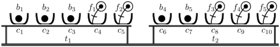
Let us see some examples. In the scene in Figure 3, there are tables, cups, balls and flowers. We use the same hypothesis as in Figure 1, i.e. we suppose that the scene is described using only unary relations (like is a table) and the binary relationsis in1,
is in2(is in/has in),is on1andis on2(is on/has on).
t1 t2 c1 c2 c3 c4 c5 c6 c7 c8 c9 c10 w b1 w b2 w b3 w b4 w b5 tj f1 f2 tj f3 tj f4 tj f5 tj
Figure 3: Another scene
As definition 1 is iterative, its application takes several steps. Each step consists in distinguishing more entities from the others: many objects are 0-confusable but few are 4-confusable. At the end, there only remain entities which are not distinguishable. These steps are the following:
1. With our definition, the tables t1and t2are 0-confusable (both are tables with five objects on them) but they are both 0-distinguishable from all the other entities. Similarly, the cups are 0 distinguishable from the flowers, the balls and the tables, and so on.
2. The cups c1, c2, c3, c6 and c7 are 1-distinguishable with the other cups since they are in relation (via has in) with entities (the balls b1. . . b5) which are 0-distinguishable from all the entities (the flowers) which are in relation via has in with the cups c4, c5, c8, c9 and c10. The cups with balls inside them are 1-distinguishable from cups with flowers inside them.
3. The tables t1and t2are 2-distinguishable one from the other: they both have five cups on them, but there do not exist three cups on t2which are simultaneously 1-confusable with c1, c2 and c3 (and conversely, there do not exist three cups on t1 which are simultaneously 1-confusable with c8, c9and c10). So, for all the orderings (c01, c02, c03, c04, c05) of T (t2, has on1) = {c6, c7, c8, c9, c10}, it is impossible to have simultaneously c1C1c01, c2C1c02and c3C1c03. Conversely, for all the orderings (c001, c002, c003, c004, c500) of T (t1, has on1) = {c1, c2, c3, c4, c5}, it is impossible to have simultaneously c003C1c8, c004C1c9and c005C1c10.
4. The cups c1, c2 and c3are 3-distinguishable from c6and c7 (and reciprocally) since they are on t1which is 2-distinguishable from t2. Similarly, the cups c4 and c5are 3-distinguishable from the cups c8, c9and c10.
5. The balls b1, b2and b3are 4-distinguishable from the balls b4and b5since they are in cups which are 3-distinguishable from the cups containing b4and b5. Sim-ilarly, the flowers f1and f2are 4-distinguishable from f3, f4and f5.
6. No 4-confusable entity is 5-distinguishable. The iteration stops.
We notice that the flowers and the balls are used to distinguish t1and t2one from the other (steps 2 and 3) and that the distinguishability of t1and t2is used to partition the flowers and the balls (step 5). But although there is a cycle, there is no infinite loop.
It can be proven that for every k ≥ 0, Ck is an equivalence relation. In addition, if two entities are k-distinguishable, then they are k0-distinguishable for every k0> k. So:
Property 1. Definition 1 yields a hierarchy on the entity set. Equivalently: K − κ is a pseudo-ultrametric3, whereK is the greatest κ(x, y).
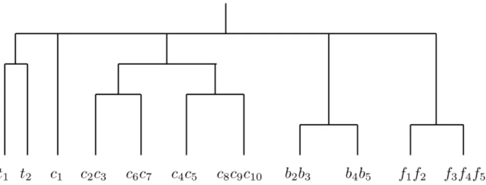
The dendrogram obtained from the example of Figure 3 is the one in Figure 4. In this example, one can see that unary properties give the first level of the hierarchy (κ = 0): from left to right, these four classes are the tables (C01 = {t1, t2}), the cups (C02 = {c1, c2. . . , c10}), the balls (C3
0 = {b1, b2. . . , b5}) and the flowers (C 4 0 = {f1, f2. . . , f5}). The use of n-ary relations give four more levels of classification.
At level κ = 1, the class C02is partitioned into C11∪C12, where C11= {c1, c2, c3, c6, c7} is the class of the cups containing a ball and C12 = {c4, c5, c8, c9, c10} is the class of the cups containing a flower.
At level κ = 2, the class C01is partitioned into C21∪ C22= {t1} ∪ {t2}.
At level κ = 3, C11is partitioned into C31∪C32, where C31= {c1, c2, c3} is made of the cups containing a ball which are on t1and C32= {c6, c7} is made of the cups containing a ball which are on t2. Similarly, C12is partitioned into C33∪C34= {c4, c5}∪{c8, c9, c10}.
At level κ = 4, C3
0 is partitioned into C41∪ C42, where C41 = {b1, b2, b3} are the elements e of C3
0 which are contained in elements of C31, i.e. C41are the balls which are in cups on t1. C2
4 = {b4, b5} is the class of the balls in cups on t2. Similarly, C04is
3d = K − κ is not an ultrametric since x 6= y does not imply d(x, y) 6= 0. In order to get an ultrametric, one can define d0(x, y) = 0 if x = y and d0(x, y) = d(x, y) + 1 otherwise.
t1 t2 c1c2c3 c6c7 c4c5 c8c9c10 b1b2b3 b4b5 f1f2 f3f4f5 . . . κ = 0 . . . κ = 1 . . . κ = 2 . . . κ = 3 . . . κ = 4
Figure 4: The dendrogram for the scene in Figure 3
partitioned into C3
4∪ C44 = {f1, f2} ∪ {f3, f4, f5} (the flowers in cups on t1and the flowers in cups on t2).
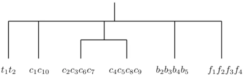
One characteristic of our ultrametric is that the distance between two entities de-pends on all of the entities in the context. So if we take out one entity, the whole hierarchy may change. In the example in Figure 3, if we take out b1and f5, we obtain the dendrograms in Figure 5 and Figure 6. One can see that the dendrograms in Figure
t1 t2 c1 c2c3 c6c7 c4c5 c8c9c10 b2b3 b4b5 f1f2 f3f4f5
Figure 5: The dendrogram for Figure 3 if b1is taken out
4, Figure 5 and Figure 6 are structurally different.
Figure 5 and Figure 6 also illustrate another characteristic of definition 1. Actu-ally, looking at the dendrogram in Figure 4, it may seem that 0-distinguishability only derives from unary properties like being a table, or being a cup, etc as it is often the case in classical taxonomy, where attributes are ordered and these ones would be con-sidered as “main” attributes. In our work, properties are not ordered: in Figure 5 and Figure 6, empty cups (c1in Figure 5 and c1, c10in Figure 6) are 0-distinguishable from not empty cups, as they are 0-distinguishable from tables and flowers. Actually, in the dendrogram of Figure 4, the class C01 is made of entities which are tables and have 5
t1t2 c1c10 c2c3c6c7 c4c5c8c9 b2b3b4b5 f1f2f3f4
Figure 6: The dendrogram for Figure 3 if b1and f5are taken out
objects on them, the class C02 is made of cups which are on something and have an object inside them, the class C03is made of balls which are in something, and the class C4
0is made of flowers which are in something.
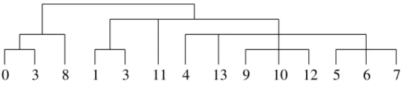
We now take as entity set E the elements of an circular array T [0 . . . n−1], with the relationsequals 1(T [i]) andis near(T [i], T [j]), which is true if 0 < |i − j| ≤ k (the operations are made modulo n). So every entity e has propertyis near1andis near2, and, for each of these properties, there are 2k tuples (made of one element) that match it with e. Some entities also have propertyequals 1. Let us consider, with n = 14 and k = 2:
T = [1, 0, 0, 1, 0, 0, 0, 0, 1, 0, 0, 0, 0, 0]
• At Step 0, E is partitioned into {T [0], T [3], T [8]} (the elements with value 1) on one hand, and the other elements on the other hand.
• At Step 1, E is partitioned into [a, b, b, a, c, c, c, c, a, c, c, 11, c, c], where a de-notes the elements which are equal to 1, b the elements which have two “neigh-bors” with value 1, c those which have one neighbor with value 1, and 11 the (unique) element all of whose neighbors have value 0.
• At Step 2, E is partitioned into [f, b, b, f, 4, e, e, e, 8, d, d, 11, d, 13]. The entity marked 13 is the unique one to have one neighbor in each of the classes a, b, c and 11; the entity marked 4 has one neighbor in a, one in b and two in c; the entity marked 8 is the only element of class a not to have a neighbor in class b, the class f is made of the other elements of class a; class d is made of the elements of class c having two neighbors in c, one in class 11 and one in a; class e is made of entities of class c which have three neighbors in class c and one in class a.
• At step 3, all entities become distinguishable: T [0] is the unique element of class f with a neighbor in class 13; T [2] is the only element of class b to have a neighbor in class 4; T [5] is the unique element of class e with a neighbor in class f ; and so on.
So, we have the dendrogram of Figure 7. Our method does not explicitly take into account symmetric relations, but it is possible to transform a symmetric relation into a
0 3 8 1 3 11 4 13 9 10 12 5 6 7
Figure 7: The dendrogram for the array T
non-symmetric one. In the last example (which corresponds to dendrogram of Figure 7), we have a symmetric relation (is near(e, e0) ⇐⇒ is near(e0, e)). Note that we have represented a fact like e is near e0byis near(e, e0) andis near(e0, e); so we have indicated that (e0) matchesis near1andis near2with e and that (e) matchesis near1 andis near2with e0. It is possible to avoid this “duplication of information” by ignor-ing propertyis near2which is equivalent to propertyis near1. This simplification is impossible for n-ary relations, and, more generally, this technique is not possible for n-ary symmetric relations (the size of the data would be multiplied by n!).
Another approach to represent a symmetric relation is the use of a fictive addi-tional entity; this is similar to the transformation of a database with n-ary relations into a equivalent database with only binary relations. For instance, a symmetric n-ary relation R, such that R({e1, e2, . . . , en}) and R({e01, e02, . . . , e0n}) are true can be rep-resented by a binary (non-symmetric) relation B with B(e1, x), B(e2, x),. . . B(en, x), B(e01, x0), . . . B(e0n, x0) true, where x and x0are additional entities. The size of the data then remains nearly unchanged, but the hierarchy is slightly changed: for instance, if e1is k-distinguishable from e01, then e2, . . . enshould be (k + 1)-distinguishable from e02, . . . e0n. But in fact, x would be (k + 1)-distinguishable from x0and e2, . . . enwould be (k + 2)-distinguishable from e02, . . . e0n.
For entities, having a property (whatever its arity is) can be seen as an attribute (an entity has or does not have this property/attribute). We can see that our method first builds a partition (the one we get with 0-distinguishability), which is the finest partition that one can get from these attributes. Then the following steps refine this partition. It is possible to obtain the first partition (the one which corresponds to 0-distinguishability) by a “classical” method using attributes. For instance, if we look at the usual classification of animals, there is an order on the attributes: the attribute hav-ing a notochord, which defines the chordates, must be considered before the attribute having a head, which defines the craniates, which is prior to having a backbone, which defines the vertebrates. Our method can be used to continue this partition by taking into account the interactions between species. If we have classified animals (using only at-tributes), then we can, for instance, classify carnivore by taking into account what kind of animals they eat, and also herbivore (depending on what animals eat them).
4
An efficient algorithm to compute the hierarchy
In this section, we give an algorithm which computes the hierarchy. An implementation
of this algorithm can be found at: https://github.com/pascalprea/Classification. This algorithm takes as entry a finite set E of entities, with the sets P(e) and T (e, pq)
for each e ∈ E and pq ∈ P(e). Sets are given with their cardinality. This algorithm relies on testing k-confusability, i.e. determining if two entities are k-confusable or k-distinguishable for a given integer k. We first study this core test.
4.1
Testing k-confusability
If k = 0, we only have to check for every property pqif |T (e1, pq)| 6= |T (e2, pq)|. This can be done in O(|P(e1)|), assuming that the sets P(e) are initially sorted. Sorting these sets takes O(nm log m) time, where n is the number of entities and m the maxi-mum number of properties an entity can have. Since our algorithm takes O(n·p·m5/2) time (p is the size of the output), sorting the sets P(e) does not increase the complexity of our algorithm.
If k > 0, we suppose that all the couples (e, e0) of entities such that κ(e, e0) < k have been already computed; so (k − 1)-confusability can be tested in O(1).
At first glance, it may seem that definition 1 yields an exponential algorithm since we have to test all the permutations of the set [1 . . . s]. But in fact, testing whether e1Dke2or not can be done in the following way:
For every property pqof P(e1):
1. We construct a bipartite graph Ge1,e2
pq = (V e1,e2 pq , E e1,e2 pq ), where: • Ve1,e2 pq = T (e1, pq) ∪ T (e2, pq)
• for t = (x1, . . . xr) in T (e1, pq) and t0= (y1, . . . yr) in T (e2, pq), {t, t0} ∈ Ee1,e2
pq if for all i ∈ [1 . . . r], xiis (k − 1)-confusable with yi.
The graph Ge1,e2
pq can be constructed in O(|T (e1, pq)|·|T (e2, pq)|·r) = O(|T (e1, pq)|
2· r). It captures how many tuples in relation with e1and tuples in relation with e2 through the same relation are pairwise confusable.
2. We check if Ge1,e2
pq admits a perfect matching (i.e. if there exists a set X of edges
such that every vertex is incident with exactly one edge of X). This can be done in O((|T (e1, pq)| + |T (e2, pq)|)5/2) = O(|T (e1, pq)|5/2) with the algorithm of Hopcroft and Karp (1973)4.
Claim 2. The entities e1ande2arek-distinguishable if and only if one graph Ge1,e2
pq
does not admit a perfect matching.
4There exists an O(n1.5pm/ log n algorithm to compute a maximal matching in a bipartite graph with n vertices and m edges (see Alt et al. 2001) but this algorithm improves the one of Hopcroft and Karp (1973) only for dense graphs. In addition, the graphs Ge1,e2
Proof. Suppose that T (e1, pq) = (t1, . . . , tk). If (t01, . . . , t0k) is an ordering of T (e2, pq) which does not satisfy the condition of Definition 1, then {{t1, t01}, {t2, t0
2}, . . . {tk, t0k}} is a perfect matching of Ge1,e2
pq ; and reciprocally.
Claim 3. Knowing (k−1)-confusability/distinguishability of every pair of entities, test-ingk-confusability can be done in O(r·m2+m5/2) time and O(m2) space, where m is the maximum number of properties an entity can have (m = maxe∈EPpq∈P(e)|T (e, pq)|),
andr the greatest arity of properties.
Proof. Let e and e0be two (k − 1)-confusable entities. For every property pqof P(e1) (= P(e2)), the algorithm first constructs the graph Ge1,e2
pq in O(|T (e1, pq)|
2· r). The graph Ge1,e2
pq can be represented by a |T (e1, pq)| × |T (e1, pq)| matrix. Then the
algo-rithm tests if Ge1,e2
pq admits a perfect matching in O(|T (e1, pq)|
5/2). AsP pq∈P(e)|T (e, pq)| 2≤ (P pq∈P(e)|T (e, pq)|) 2andP pq∈P(e)|T (e, pq)| 5/2 ≤ (P pq∈P(e)|T (e, pq)|) 5/2, the result follows.
One generally considers only properties with small arity: a property of arity > 10 is something very rare. In addition, if r can not be neglected, it has also to be considered when evaluating the size of the instance of the problem; not neglecting r is equivalent to multiplying both the size of the instance and the computation time by r. So we will consider r as a constant.
4.2
The complete algorithm
We now give the entire algorithm. Its output is a hierarchy H, given as a set of nodes; each node corresponds to a class (i.e. a subset of E) and is given by a triple made of:
• Its representative: an entity of the class corresponding to the node.
• Its depth in the dendrogram (we have fixed the depth of the root to be −1, so, if the depth of a class C is k, then two elements of C are k-confusable, and elements of C are k-distinguishable from all the entities which are not in C). • Its father, i.e. the smallest class strictly containing it, which is given by a couple
(representative, depth). There may be many classes with the same representative (and many with the same depth), but a couple (representative, depth) is charac-teristic for exactly one class.
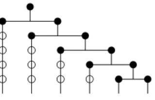
We call k-class a maximal set of entities which are pairwise k-confusable. In the dendrogram in Figure 4 one can see that {b1, b2, b3, b4, b5} is a 0-class. It is also a 1-class, a 2-class and a 3-class. In the resulting hierarchy H, {b1, . . . b5} will only be considered as a 0-class, but during the progress of the algorithm, {b1. . . b5} will also be considered as a 1-class, a 2-class and a 3-class. A k-class which is not a class of H corresponds to a (k − 1)-class which has not been subdivided at step k. So every k-class is equal to a class of H. The total number of k-classes can be much larger than the number of classes in H. For instance, in a dendrogram like the one in Figure 8 with n = 6 leaves, there are 2n − 1 = 11 “real” classes (the black circles), but the total number of k-classes is n(n + 1)/2 = 21 (the white circles represent the k-classes
which are not classes of H). We will see later that, although our algorithm considers all the k-classes, its complexity does not depend on the number of k-classes but is linear in the number of classes of H. The main variables used by our algorithm are the
t t t t t t t t t t t d d d d d d d d d d
Figure 8: A dendrogram with n leaves, 2n − 1 classes and n(n + 1)/2 k-classes
following:
• The integer k denotes the steps of the algorithm. At step k (each step goes from line 4 to 24), we look for k-distinguishability and construct all the k-classes. • At the end of step k, Rep[k] is the set of the representatives of all the k-classes.
If e and e0 are in Rep[k], eDke0, and if e /∈ Rep[k], ∃e0 ∈ Rep[k] such that eCke0.
• Sets[k] is an array indexed by the set E of all entities. At the end of step k, for each entity e in Rep[k], Sets[k][e] is the k-class which admits e as a representa-tive. If e is not a representative, Sets[k][e] is not defined and is not used. Sets does not need to be initialized.
• OppSets[k] is an array indexed by the set E of all entities. If e ∈ Sets[k][e0], then OppSets[k][e] = e0. Equivalently, at the end of step k, for each entity e in E, OppSets[k][e] is the representative of the k-class containing e. We will see that, at step k, OppSets[k − 1] is already computed; it is thus possible to test (k − 1)-confusability in O(1) (eCk−1e0if and only if OppSets[k − 1][e] = OppSets[k −1][e0]). So testing k-confusability at step k can be done in O(m5/2) time and O(m2) space.
• Depth is an array indexed by E. At step k, for every entity e which is represen-tative of one or many classes of H of depth ≤ k, Depth[e] is the greatest depth of these classes. Equivalently, Depth[e] is the depth of the smallest (yet computed) class of H containing e. If e is not the representative of a class, Depth[e] is not defined. Depth does not need to be initialized.
• Continue indicates if, at step k, some classes are created. If it is not the case, the algorithm stops.
We now detail how Algorithm 1 works.
At line 2, the algorithm creates the root of the hierarchy: a unique class containing all the elements of E, whose representative is e1and depth −1.
Algorithm 1: HIERARCHYCOMPUTATION
Input: A set E = {e1, . . . en} of entities. Output: A hierarchy H on E.
1 begin
2 H ← {(e1, −1, ∅)} ; Rep[−1] ← e1; Sets[−1][e1] ← E ; Depth[e1] ← −1 ;
3 k ← 0 ; Continue ← True ; 4 while Continue do 5 Rep[k] ← ∅ ; 6 foreach e ∈ Rep[k − 1] do 7 T emp ← Depth[e] ; 8 CurrentRep ← ∅ ;
9 foreach e0∈ Sets[k − 1][e] do
10 N ew ← True ;
11 foreach e00∈ CurrentRep do
12 if e0Cke00then
13 Sets[k][e”] ← Sets[k][e”] ∪ {e0} ;
14 OppSets[k][e0] ← e” ; N ew ← False ;
15 if N ew then
16 CurrentRep ← CurrentRep ∪ {e0} ;
17 Sets[k][e0] ← {e0} ; OppSets[k][e0] ← e0;
18 Depth[e0] ← k ; H ← H ∪ {(e0, k, (e, T emp))} ;
19 if CurrentRep = {e} then
20 H ← H \ {(e, k, (e, T emp))} ; Depth[e] ← T emp ;
21 Rep[k] ← Rep[k] ∪ CurrentRep ;
22 Continue ← (|Rep[k]| 6= |Rep[k − 1]|) ;
23 Delete (Rep[k − 1]) ; Delete (Sets[k − 1]) ; Delete (OppSets[k − 1]) ;
24 k ← k + 1 ;
25 foreach e ∈ Rep[k − 1] do
26 foreach e0∈ Sets[k − 1][e] do
27 H ← H ∪ {(e0, k, (e, Depth[e]))} ;
28 end
The k-classes are subclasses of (k − 1)-classes. So the algorithm, on lines 6 and 9, will consider the (k − 1)-classes independently (instead of considering all the elements of E “at the same time”).
CurrentRep is the set of the representatives of the (already known) subclasses of the (k − 1)-class of e. For every entity e0 of Sets[k − 1][e], the algorithm checks if e0 is k-confusable with a representative of a class. If e0 is k-confusable with a rep-resentative e00, the algorithm adds e0 to the k-class of e00, i.e. to Sets[k][e00]. If e0 is k-distinguishable with all the (already known) representative, then, at line 15, N ew is true and a new k-class is created with representative e0(lines 16—18). This is always
the case for the first element of Sets[k − 1][e].
Before the loop 9—18, CurrentRep is empty. Once computed, it is added to the set Rep[k] (line 21).
On lines 19 and 20 is treated the case when the (k − 1)-class C of e is not parti-tioned at step k; in this case, C is also a k-class and CurrentRep contains exactly one element, the representative of C. We can suppose that each time the algorithm goes through a set, it does it in the same order, so the representative of C, as a k-class, is also e. C must not appear as a k-class in H. So the algorithm takes it out of H and gives the value it had before lines 9—18 to Depth[e]. This value has been loaded into T emp at line 7.
On line 22, the algorithm checks if “something has been done at step k”, i.e. if there are more k-classes than (k − 1)-classes. If it is not the case, no other step is necessary. After step k, the algorithm will not use what has been done at step k − 1. So Rep[k − 1], Sets[k − 1] and OppSets[k − 1] are deleted in order to minimize the memory used by the algorithm.
On lines 25—27, each entity is assigned to the smallest class containing it; the hierarchy H is then complete.
Property 2. Algorithm 1 runs in O(n + m2) space and O(n · p · m5/2) time in worst case, wheren is the number of entities, p is the number of classes in H (p < 2n) and m is the maximum number of properties an entity can have.
Proof. The algorithm uses 9 sets5 of elements (Rep[k − 1], Rep[k], Sets[k − 1], Sets[k], OppSets[k − 1], OppSets[k], Depth, CurrentRep and H) which are all of size O(n). It also has to build graphs with 2m vertices, but only one at a time. So it runs in O(n + m2) space.
The time complexity of Algorithm 1 depends on the number of tests “if e0Cke00” (line 12), where e0is an entity and e00a representative of a k-class (we recall that each of these tests takes O(m5/2) time; in addition, what the algorithm does in each case takes a constant amount of time). We prove that, for each entity e, the number of these tests is O(p).
Let e be a fixed entity. At Step k, e is only “compared” with subclasses of the (k − 1)-class to which it belongs (lines 6, 9 and 11).
We first give an upper bound of the number of times e is compared with a class it does not belong to. For any k, all the k-classes to which e is compared while not belonging to them are disjoint. Moreover, since all these k-classes are subclasses of the (k − 1)-class of e, the (k − 1)-classes not containing e and to which e is compared are disjoint from the compared k-classes not containing e. All are subclasses of the (k − 2)-class of e, so the compared (k − 2)-subclasses not containing e are disjoint from the compared k-classes and (k − 1)-classes. Thus all the classes not containing e to which e is compared are disjoint. Since every class is equal to a class of H, e is compared with at most p − 1 classes not containing it.
We now give the number of comparisons between e and a class to which it belongs. For every k ≤ K, e is in exactly one k-class. At each step of the algorithm (except the
last one), at least one class is divided and so two or more classes of H are “created”. So K ≤ p and e is compared with at most p classes containing it.
Each entity is compared with O(p) classes, so there are O(n · p) tests of line 12 and Algorithm 1 runs in O(n · p · m5/2) time (lines 25—27 take O(n) time and do not change the overall complexity).
The bound O(np) for the number of comparisons can be reached, for instance if all the entities are 0-distinguishable. On the contrary, if the hierarchy is a balanced binary tree, at each step, every entity is compared with at most two classes; so the total number of comparisons is O(n log p).
4.3
Tests on large sets of entities
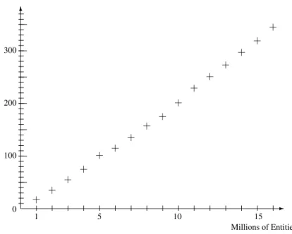
Today, one often has to treat huge data sets, i.e. millions of entities. So, although our algorithm has a polynomial time and space complexity, it is interesting to test it on large data sets and so, we have tested our algorithm on data sets up to 10 million entities. We do not pretend that our implementation is the best possible (the program is written in Python, which is an interpreted language; more precisely, these tests ran in Python 2.7 on a 16 Intel Xeon X5560 at 2.8 GHz computer with 48 Gb RAM. The computer has 16 processors, but only one was used for these tests); these tests are just “feasibility tests”.
The construction of the entity sets is similar to what was done for the last example of section 3: we have generated large data sets with {0,1}-arrays of size 1 million, 2 millions, . . . 16 millions . More precisely, the arrays are random arrays (each cell has probability 0.5 to be one). The relations areequals 1(e) andis near(e1, e2) (two entities T [i] and T [j] are “near” if 0 < |i−j| < 3). Since relationis nearis symmetric, we only consider propertyis near1. For each entity e, there are four tuples that match
is near1with e. For such data sets, all the entities are distinguishable, so p ≈ n. This is the worst case for our algorithm. We obtained the results of Figure 9.
• The amount of memory used is approximatively 2.5 GigaBytes per million enti-ties.
• The computation time grows slower than np (the time needed to treat 5 million entities is smaller than 25 times the time needed to treat one million), which is the theoretical complexity. Actually, the computation time also depends on the depth of the hierarchy. For arrays used in this test, this depth is < 15 (two entities are 15-confusable if two balls of radius 30 are identical; there are 261possible such balls).
So, we can see that our algorithm is able to treat large data sets. The classification method that we propose in this paper is thus applicable for “real world” applications.
-6 Millions of Entities Time (min) 0 100 200 300 1 5 10 15 + + + + + + + + + + + + + + + +
Figure 9: Time needed to treat large entity sets
5
Test on Fisher’s iris data set
Our method is, basically, a discrimination method: we detect differences between en-tities which are, a priori, similar (since they are 0-confusable). When we apply it on a randomly generated entity set as in Section 4.3, we get a final partition made of sin-gletons. On the contrary, when applied on real data, our method may yield a partition made (at least partly) of “large” sets. In this case, we can say that there is a “structure” inside this data set.
We have tested our method on the Fisher iris data set (from Fisher 1936). This data set is made of 150 iris flowers: 50 iris i.setosa, 50 iris i.versicolor and 50 iris i.virginica. Each flower is given with four parameters: the length and width of the petal and the sepal. It is very easy to recognize the i.setosa among the iris: they all have a petal width ≤ 0.3 while all the others have a petal width ≥ 1. There is not such an easy separation between the i.versicolor and the i.virginica. In Figure 10 is shown the result of a Principal Component Analysis of this data set.
In order to apply our method to this data set, we first have to define relations be-tween iris. We do that in the following way:
1. We normalize the four parameters: the average value is 0 and the standard devi-ation is 1.
2. Given a threshold h, we say that two iris are close if they have two parameters which differ by less than h; so we have one binary relation: is close (iris1, iris2)
-3 -2 -1 0 1 2 3 -2 -1 0 1 2 1st component 2n d co mp on en t
Figure 10: The result of a PCA on Fisher’s iris; The i.setosa are marked with a circle, the i.versicolor with a triangle and the i.virginica with a cross.
and one property is close1(the properties is close1and is close2are equiva-lent). Actually, we build a graph with 150 vertices (the iris) and a number of edges that will depend on h.
By applying our method, we get the following results:
• With h = 1, no information or structure can be detected among the iris: the final partition of the iris set is made of 130 small classes (the greatest is of size 5). • With h = 1/2, we “recognize” the i.setosa: the final partition is made of one
class with 39 elements (all i.setosa) one class with 5 elements (all i.setosa), two pairs and singletons.
• With h = 2, we recognize the i.versicolor: the final partition is made of one class with 51 elements (47 i.versicolor and 4 i.virginica), one with 6 elements (all i.setosa), 8 pairs and singletons.
These results can be interpreted in the following way:
• With threshold h = 1/2, we link each iris with its close neighbors (the standard deviation for each parameter is 1). The i.setosa form a dense class, which is well separated from the other iris. So each i.setosa has many neighbors among the i.setosaand none among the other classes. Actually, the “large” class is made of iris which have 49 neighbors, 38 of them having 49 neighbors. The other i.setosa have a little less than 49 neighbors (among which 38 have 49 neighbors).
• The threshold h = 2 is approximatively the radius of the set. We recognize the i.versicolorbecause they are in central position among the iris. The large class is made of the iris which are neighbors with all the other iris.
6
Related works and perspectives
Some previous works deal with n-ary functions on entities (see Agarwal et al. 2005; Diatta 2004; Pr´ea 1994), but their goal is to define a measure on sets which is based on many points, and then to apply metric methods. Basically, our method is not metric: we do not use a n-metric to classify, but we build an ultrametric from boolean (n-ary) functions.
Although the tests have shown that it is possible to treat huge data sets, treating efficiently such data sets would require some improvements; a promising one would be parallel programming. Parallelisation is possible, since at each step, the same treat-ment is independently applied on all entities (more precisely, at each couple (entity, representative) of its class).
A characteristic of the ultrametric we build is its dependence on the entire set of en-tities, or, equivalently, the instability of the obtained classification, which is illustrated in Figures 4, 5 and 6. If we consider a social network with the relation is friend with, such an instability is critical: people often add, and sometimes remove, friends. In ad-dition, for such a network, distinguishing between someone who has 511 friends, and another one who has “only” 497 is not pertinent. Actually, this precision is the cause of the instability. This precision is also better for discriminate/separate than for clas-sify/put together. One way to correct these two defaults would be to use an imprecise measure, like fuzzy sets (see Zadeh 1965) to estimate the number of tuples matching a property with an entity. For instance, with less precision when analysing the Fisher iris, with threshold h = 1/2, we can characterize the i.setosa as the iris which have around 49 neighbors, each of these neighbors also having around 49 neighbors, and with threshold h = 2, we can characterize the i.versicolor (plus around 8 i.virginica) as the iris having nearly 149 neighbors.
References
[1] AGARWAL, S., LIM, J., ZELHIK-MANOR, L., PERONA, P., KRIEGMAN, D. and BELONGIE, S. (2005),“ Beyond Pairwise Clustering”, in Proceedings of the IEEE Computer Conference on Computer Vision and Pattern Recognition, Piscataway, IEEE Computer Society, vol. 2, pp 838-845.
[2] ALT, H., BLUM, N., MEHLTON, K. and PAUL, M. (2001), “Computing a max-imal cardinality matching in a bipartite graph in time O(n1.5pm/ log n)”, In-formation Processing Letters, 37 (4): 237-240.
[3] BARTHELEMY´ , J.-P. and GUENOCHE´ , A. (1991), Trees and Proximity Repre-sentations, Wiley.
[4] BUFFON, G.-L. LECLERC DE (1749), Histoire Naturelle, G´en´erale et Particuli`ere, avec la Description du Cabinet du Roy, available at www.buffon.cnrs.fr.
[5] CROITORU, M. and DEEMTER, K. VAN (2007), “A Conceptual Graph Ap-proach to the Generation of Referring Expressions”, in Proceedings of the Inter-national Joint Conference on Artificial Intelligence, Hyderabad, Morgan Kauf-man, pp 2456-2461.
[6] DALE, R. (1989), “Cooking up Referring Expressions”, in Proceedings of the Twenty-Seventh Annual Meeting of the Association for Computational Linguis-tics, Vancouver, Association for Computational LinguisLinguis-tics, pp. 68-75.
[7] DEEMTER, K. VAN(2002), “Generating Referring Expressions: Boolean Ex-tensions of the Incremental Algorithm”, Computational Linguistics, 28(1):37-52.
[8] DEEMTER, K.VANand KRAHMER, E. (2006), “Graphs and Booleans: On the generation of referring expressions”, in Computing Meaning : Volume 3 (Studies in Linguistics and Philosophy), H. Bunt and R. Muskens Eds., Springer, pp 397-422.
[9] DIATTA, J. (2004), “A Relation Between the Theory of Formal Concepts and Multiway Clustering”, Pattern Recognition Letters, 25:1183-1189.
[10] FISHER, R.A. (1936), “The use of multiple measurements in taxonomic prob-lems”, Annals of Eugenics, 7 (2): 179–188.
[11] GARDENT, C. (2002), “Generating Minimal Definite Descriptions”, in Proceed-ings of the 40th Annual Meeting of the Association for Computational Linguis-tics, Philadelphia, Association for Computational LinguisLinguis-tics, pp 96-103. [12] GORDON, A.D. (1999), Classification, Chapman & Hall.
[13] HOPCROFT, J.E. and KARP, R.M. (1973), “An n5/2Algorithm for Maximum Matchings in Bipartite Graphs”, SIAM Journal on Computing, 2(4):225-231. [14] JARDINE, N. and SIBSON, R. (1971), Mathematical Taxonomy, Wiley. [15] KHAN, I.H., DEEMTER, K.VAN, RITCHIE, G., GATTA. and CLELAND, A.A.
(2009), “A Hearer-Oriented Evaluation of Referring Expression Generation”, in Proceedings of the 12th European Workshop on Natural Language Generation, Athens, Association for Computational Linguistics, pp. 98-101.
[16] KRAHMER, E., ERK, S.VANand VERLEG, A. (2003), “Graph-based Genera-tion of Referring Expressions”, ComputaGenera-tional Linguistics, 29(1):53-72. [17] LINNE´, C. VON (1735), Systema Naturæ, available at
[18] MITCHELL, M., (2009), “Class-Based Ordering of Prenominal Modifiers”, in Proceedings of the 12th European Workshop on Natural Language Generation, Athens, Association for Computational Linguistics, pp 50-57.
[19] OSBORNE, M.J. (2009), An Introduction to Game Theory, Oxford University Press.
[20] PREA´ , P. (1994), “A Generalization of the Diameter Criterion for Clustering”, in New Approaches in Classification and Data Analysis, E. Diday, Y. Lechevallier, M. Schader, P. Bertrand and B. Burtschy Eds., Springer-Verlag, pp 257-262. [21] ROLBERT, M. and PREA´ , P. (2009), “Distinguishable Entities: Definitions and
Properties”, Proceedings of the 12th European Workshop on Natural Language Generation, Athens, Association for Computational Linguistics, pp 34-41. [22] ZADEH, L.A. (1965), “Fuzzy Sets”, Information and Control, 8:338-353.