Categories and String Diagrams for Game Semantics

(1)

HAL Id: tel-02147264

https://tel.archives-ouvertes.fr/tel-02147264

Submitted on 4 Jun 2019

HAL is a multi-disciplinary open access

archive for the deposit and dissemination of

sci-entific research documents, whether they are

pub-lished or not. The documents may come from

teaching and research institutions in France or

L’archive ouverte pluridisciplinaire HAL, est

destinée au dépôt et à la diffusion de documents

scientifiques de niveau recherche, publiés ou non,

émanant des établissements d’enseignement et de

recherche français ou étrangers, des laboratoires

Categories and String Diagrams for Game Semantics

Clovis Eberhart

To cite this version:

Clovis Eberhart. Categories and String Diagrams for Game Semantics. Computer Science and Game

Theory [cs.GT]. Université Grenoble Alpes, 2018. English. �NNT : 2018GREAM091�. �tel-02147264�

(2)

THÈSE

Pour

obtenir le grade de

DOCTEUR

_DE

LA COMMUNAUTÉ UNIVERSITÉ

GRENOBLE

ALPES

Spécialité

: Mathématiques

Arrêté ministériel : 25 mai 2016

Présentée par

Clovis

_Eberhart

Thèse

dirigée par Tom Hirschowitz

préparée

au sein du Laboratoire de mathématiques

et

de l’Ecole Doctorale de Mathématiques, Sciences et Technologies

de

l’Information, Informatique

Catégories

_{et diagrammes de}

cordes

_{pour les jeux concurrents}

_{and String Diagrams for}

Concurrent

_{Game Semantics}

Thèse

_{soutenue publiquement le 22 juin 2018,}

devant

le jury composé de :

Mr.

Martin Hyland

Professor, Department of Pure Mathematics and Mathematical Statistics, Univer-sity_{of Cambridge, Président}

M. Samuel Mimram

Maître_{de conférences, LIX, École polytechnique, Rapporteur}

M. Pierre-Louis Curien

Directeur de recherche CNRS, IRIF, Université Paris Diderot, Examinateur

M. Vincent Danos

Directeur_{de recherche CNRS, Département d’informatique, ENS, Examinateur}

M. Paul-André Melliès

Chargé_{de recherche CNRS, IRIF, Université Paris Diderot, Examinateur}

M. Tom Hirschowitz

(3)

(4)

Thanks

I would like to extend my thanks to all the people I have shared these few years with. To Tom Hirschowitz, my PhD supervisor, whose vast knowledge of category theory and abstract way of thinking never ceased to amaze me, and who has been more of a colleague with whom I had a fruitful collaboration than someone who simply supervised my work. To Krzysztof Worytkiewicz, who was my official supervisor for the first two years of my PhD, even though we worked on different topics. To the members of the LIMD team, past or present, especially those with whom I have interacted the most : Pierre for all the fascinating math problems and anecdotes about computer science, Jaco for his spirit, humour, and common sense, Christophe for his enthusiasm and ability to always randomly generate conversation topics, and Xavier for his common interests in food and a certain Québecois humourist. To the PhD students at LAMA, either past or present : Rodolphe, Pierre, Florian, Lars, Marion, Boulos, Lama, Rémy, Charlotte, Suelen, and all those I have forgotten to mention. More generally, I would like to thank the whole LAMA laboratory for the wonderful years I have spent there. I would like to (unironically) thank the administration at MSTII (and more generally any person who had to deal with me from an administrative point of view) for their patience. Finally, I would like to thank the reporters – Marin Hyland and Samuel Mimram – and examiners – Pierre-Louis Curien, Vincent Danos, and Paul-André Melliès – for reading this manuscript, making enlightening comments about it, and giving me some pointers for future research directions.

(5)

Introduction

In recent years, there has been increasingly more focus on concurrent program-ming, following the increase in the average number of cores in a processor and the rise of distributed computing. However, many programs are still unable to use several cores simultaneously, as concurrent computing is much less intuit-ive than classical computing. One way to make concurrent computing simpler could be to design languages speciﬁcally for concurrency, which requires under-standing the basic notions behind it. For example, an appealing aspect of func-tional languages (admittedly not to the average programmer) such as OCaml or Haskell is that they are built on well-understood theories, and these languages can thus be used to test the eﬀectiveness of functional programming techniques on real problems, rather than academical ones. Once these techniques have proved useful, functional programming paradigms can then be added to “main-stream” programming languages such as Python or C++, where they can be used to solve some problems more easily. This work is a contribution to concur-rent game semantics, a research area that uses game semantics to understand concurrency better.

1.1 Semantics of Programming Languages

Semantics of programming languages (or simply semantics for short) is a ﬁeld of computer science whose goal is to assign mathematical meaning to programs. Indeed, a term of a language is just a sequence of symbols, which in itself carries no meaning, and whose meaning is only understood in the context of a partic-ular language. The idea is thus to build mathematical models of programming languages to prove properties of programs.

There are several reasons why one would want to give a mathematical mean-ing to programs: to prove that programs written in a particular language have a certain property, to prove that a particular program has the intended behaviour, to prove that it terminates within a reasonable amount of time, to prove that two programs have the same behaviour... It is also interesting to study pro-gramming languages in light of their link to logics, given by the Curry-Howard isomorphism [95]. In its most basic form, it states that types A of a program-ming language can be seen as propositions JAK of a logic and vice versa. But the interesting part is: programs of type A in the language correspond to proofs of

(9)

JAK in the logic. The correspondence is even ﬁner than this, stating that com-position of programs correspond to cuts in the logic (a cut is a step in a proof that does not prove anything new, for example, introducing a lemma). Finally, it states a dynamic correspondence between proofs and programs, in the sense that normalisation (execution) of a program corresponds to cut-elimination in the proof (a process that turns a proof into a proof of the same proposition, but without cuts, and which basically corresponds to inlining all the lemmas introduced in the proof). Semantics is thus a way to understand logic better, and vice versa.

1.1.1 An (Outdated) Map of Semantics

Let us give a slightly outdated view of semantics (we will then see that the landscape of semantics is more complex today).

Semantics comes in several diﬀerent ﬂavours, usually depending on the kind of property that one wishes to prove. It has two main branches: operational semantics, which describes programs as some kind of machine, and denotational semantics, which describes programs as well-known mathematical structures. Operational Semantics

Operational semantics is probably the representation of programming languages that is closest to the intuitions programmers have about them. It describes programs as sequences of instructions to be executed by a kind of machine. This is indeed very close to what happens inside a computer, though the set of instructions used in operational semantics is meant to abstract away some of the complexity.

There are different forms of operational semantics, but they all reflect the idea described above. Maybe the most widespread one relies on labelled trans-ition systems (or LTSs), which are basically graphs whose vertices are the set of all possible program states and whose edges correspond to execution steps of a program that starts in a certain state and ends in another one. Giving reduction rules for formal languages (such as the λ-calculus [11] or the π-calculus [85]) is exactly defining an LTS whose vertices are the terms of the language and edges are possible reductions. For example, here is a very simple LTS for the λ-calculus: M’ (λx.M)N → M[N/x] M → M ′ M N→ M′N N→ N′ M N→ MN′ . Some LTSs are based on abstract machines [63]. As the name indicates, they are in some sense even closer to the idea of a machine executing a sequence of instructions, usually executing a program or term within a context called a stack, and both the term and the stack may be modified by the various instructions the machine executes. For example, the machine may stack the arguments of an application and then unstack them when they are used, which is exactly what this machine for the λ-calculus does:

M NȂ π → M Ȃ N ∶∶ π (λx.M) Ȃ N ∶∶ π → M[N/x] Ȃ π.

Here, π is the stack (a sequence of λ-terms), the ﬁrst rule says that the machine stacks the argument when it encounters an application, and the second rule

(10)

says that the machine pops an argument and performs the substitution when it encounters an abstraction.

Denotational Semantics

While the interpretation of a program is typically close to its syntax in oper-ational semantics, denotoper-ational semantics represents programs as well-known mathematical structures. The idea is to interpret a type A as a space JAK of some kind (for example, topological spaces) and functions of type A → B as morphisms from JAK to JBK (in the case of topological spaces, morphisms would be continuous functions).

One such semantics is given by Scott domains [93]. Basically, a Scott domain is an ordered set that represents “information” about objects of a certain type: x< y means that y holds more information about what it is describing than x. For example, the Scott domain for integers has a bottom element (no information about the integer is known) and an element for each integer (greater than the bottom element, but incomparable to one another) that represents the fact that we know the value of the integer:

0 1 2 3 . . . .

A morphism between two Scott domains is basically a monotone function. In terms of programs, this means that, the more information a program has about its input, the more information it may produce about its output. For example, the denotation (interpretation) of a program that computes the predecessor but does not terminate on 0 would be the function that maps and 0 to , and n> 0 to n − 1.

A dentoational semantics should respect several properties in order to be considered “good”. Let us assume that we are given a relation on terms that ex-presses whether two terms have the same behaviour (for example, whether they return the same result given the same arguments). The first and most obvious property that a dentoational semantics should verify is soundness, i.e., that two programs that have different behaviours must have different denotations. There is not much that can be said about a semantics that does not even verify this property. The second one is completeness, i.e., that two programs that have the same behaviour must have equal denotations. When both properties above hold, we say that the model is fully abstract. This is an interesting property because studying equality in the model is enough to deduce behavioural equivalence of terms. Another important property is whether the (compact) definability result holds in the model, which means that each (compact) element of the model is the interpretation of a term (we also say that the model is denotationally complete).

Finally, a crucial property of denotational semantics is compositionality, i.e., that the denotation of a program can be deduced from those of its sub-programs. For example, for the λ-calculus, we would want to be able to compute JMNK from JMK and JNK. If we see M as a function of type A→ B whose argument is an N of type A, we want to deﬁne JMNK = JMK (JNK), which is indeed

(11)

compositional. (The actual deﬁnition is slightly more involved because we want to interpret typing derivations rather than terms.)

1.1.2 Semantics Today

Today, there is a whole array of models of programming languages, and some of them may be seen both as denotational and operational. A prime example is game semantics: it may be seen as a denotational semantics because it inter-prets programs as strategies on a general notion of game, but strategies actually encode the interaction between the program and its environment, making the model very dynamic, and in many cases (ﬁnite) strategies are in bijection with normal forms, making the model very close to syntax, which are some reasons why it is also close to operational semantics.

Nowadays, the meanings of denotational and operational semantics have shifted from their original definitions to take a broader sense. For example, some people do not consider models to be denotational unless they are fully abstract (more precisely, unless they are complete, because models that are not even sound can hardly be called models), but most people consider them to be denotational to some degree. Some models are definitely considered denotational (such as Scott domains) and others definitely not (such as LTSs). Between these two extremes, there is a continuum of models that may be considered more or less denotational, based mainly on two criteria. The first criterion is “how mathematical” the structures used to interpret types and programs are: more common ones (say, topological spaces or vector spaces) will give models that are considered more denotational than models based on less common structures, and ad hoc structures (such as LTSs or categories derived from the language’s syntax) are not denotational at all. The second criterion is whether the model enjoys “good” features (such as full abstraction) or not: those that do tend to be considered more denotational than those that do not. In both respects, game semantics lies at an intermediate point: strategies are not as common as vector spaces or topological spaces, but they are not ad hoc structures either, and while the model is not fully abstract, it is compositional and syntax-independent, and an extensional quotient gives a fully-abstract model.

Similarly, the notion of operational model has also evolved over time. A model used to be considered operational when it was derived from the syntax of a language, such as LTSs. Today, there is another dimension to operational models: a model is considered operational if it is dynamic, i.e., the execution of the program can be recovered from its interpretation.

Maybe the distinction between operational and denotational models has be-come too coarse nowadays, and should be reﬁned into diﬀerent axes on which each model may be placed: models based on mathematical structures (topolo-gical spaces) versus syntactic models (LTSs), static models (functions) versus dynamic models (strategies), or intensional models (equality is based on reduc-tion) versus extensional models (equality is based on observareduc-tion), etc.

1.2 Game Semantics

We have discussed both operational and denotational semantics (while trying to stay at a rather informal level) and have claimed that game semantics may

(12)

be seen as both. We here discuss game semantics, which will be at the heart of this work, in a bit more detail.

1.2.1 The Birth of Game Semantics

Game semantics was ﬁrst born in the realm of logic, in the form of dialogical logic [75]. Dialogical logic expresses proofs of a formula as two entities debating whether a formula is true or not: Proponent, who tries to prove that the formula is true, and Opponent, who tries to prove that it is false. This formal game is the description of a dialogue between two (rational) individuals would have when debating whether a mathematical proposition holds or not: they both defend their case until one of them is convinced they were wrong. A formula is true when Proponent has a winning strategy in a certain game played on the formula, which amounts to always managing to convince Opponent that the formula is true, no matter the objections that are raised.

It was then introduced into the world of programming languages under the name game semantics by a long series of authors, notably Berry and Curien [13] (under the name of sequential algorithms), who were the ﬁrst to use the idea of interaction in semantics and gave a sequential, denotational semantics of a higher-order language, Blass [14, 15], who exhibited links between game se-mantics and linear logic [41], Joyal [58], who was the ﬁrst to build a category of games and strategies, Coquand [23]; who linked game semantics to the dynamics of cut elimination (and thus to evaluation of programs), Abramsky, Jagadeesan, and Malacaria [6], and Hyland and Ong [56] and Nickau [87], who built the most well-known frameworks for game semantics today: AJM and HON games.

The most basic idea comes straight from dialogical logic: types are inter-preted as formal games (formulas) and programs as the interactions they may have with the environment (proofs of the formulas). In slightly more detail, types are interpreted as games (sometimes called arenas) on which notions of plays are built. Plays represent all the possible interactions an element of a given type may have with its environment. Programs of a certain type are then interpreted as strategies in that game, i.e., sets of plays satisfying some con-straints. These plays are the interactions the programs may actually have with the environment: if σ is the interpretation of a program P , then a play p belongs to σ if and only if P may interact with its environment according to p. Here, however, strategies are only used to compute values, and there are no “winning” strategies.

For example, the plays for natural numbers could be sequences of the form (q N)∗_{, where q is a move in the game representing the environment asking (q}

stands for “question”) for the value of the number, and N is any natural number, which represents the program answering the value of the number. The strategy corresponding to a counter that increases by 1 each time it is called would consist of all plays of the form q 1 q 2 . . . q n. For functions of type int → int, the set of plays could be of the form(qr(qlNl)∗ Nr)∗, where qris a move that represents

the environment asking the function for the result (r stands for “right”, as in the right-hand side of int → int) of its computation, Nr represents the function

returning the value of its result to the environment, ql represents the function

asking for the value of its argument (l stands for “left”), and Nl represents the

(13)

corresponds to the environment asking the function for the value of its result a certain number of times, and each time the function asks for the value of its argument a certain number of times before returning its result. For example, the strategy associated to the successor function would be the set of plays of the form qr ql n1l (n

1_{+ 1)}

r. . . qr ql nkl (nk+ 1)r. The exact structure of plays

depends on the type of game semantics that we are considering, but this gives a good idea of what plays and strategies look like.

Two other ideas are also present in most game models today. The ﬁrst one is innocence, which is that pure programs (those programs that only use purely functional features) are interpreted as innocent strategies. The behaviour of these strategies is based on limited information about what has happened in the play until now. This information basically encodes the part of the interaction between the program and its environment that has led to the current situation. In particular, a function may only rely on the current function call. For example, the strategy for the counter program above is not innocent because it needs to know what it answered last time, and that the only part an innocent strategy would be allowed to rely on is qr (and the counter is indeed impure). On the

other hand, the strategy associated to the successor function is innocent because its answer (nk+ 1)

ronly depends on nkl, and nothing else.

Finally, an important aspect of game semantics is how strategies are com-posed. Indeed, game models are compositional, and there is in particular a no-tion of composino-tion of strategies that corresponds to composino-tion of programs. It is defined in two steps called parallel composition and hiding. Parallel com-position lets both strategies interact. To define it, we need to define a notion of “plays” on three games: assume that σ is a strategy on the games A and B and τ a strategy on the games B and C, then we want the parallel composite σ∥τ to be a strategy on the games A, B, and C. The parallel composite then accepts a play on (A, B, C) if and only if its projection to (A, B) is accepted by σ and its projection to (B, C) is accepted by τ. The idea is that σ and τ communicate on the B game. The second step, hiding, consists in erasing the B game to make the composite a strategy only on the games A and C.

As we have already mentioned, game models may be considered denotational because they interpret programs as strategies, which are subsets of general struc-tures. On the other hand, they are operational because strategies are often in bijection with normal forms, and the interpretation of a program is exactly the interactions it may have with the environment, which makes these models close to the dynamics execution.

1.2.2 The Rich World of Game Models

Today, there are many game semantical models based on various ideas that make the game semantical landscape very diverse. What is probably considered the ﬁrst game semantical model was built by Blass [14, 15]. In this setting, a game is described as the tree of its positions, and plays are branches of that tree. In the case of functions of type A→ B, plays may be seen as a branch in A and a branch in B. A strategy is basically a choice of move to play at each node. Composition of strategies is deﬁned by playing on three trees at the same time (then hiding what happens on the middle tree). However, composition is not associative (because of a technical problem with polarity of moves).

(14)

The first game semantical models that have become popular and whose vari-ants are still used today are AJM games [6] and HON games [56], which were both invented in the 1990s. AJM games define games as sets of moves together with a condition that tells when a sequence of moves is a valid play. HON games define games as a structured set of moves and plays as structured sequences (the exact structure is beyond the point here). Both models then define strategies as prefix-closed sets of plays and composition of strategies as parallel composition plus hiding, where both operations are defined in similar ways in both models. Today, there are many variants of HON and AJM games, invented for differ-ent purposes. First of all, a number of variations on these games (that impose further conditions on sequences to be valid plays) are described in Harmer’s PhD thesis [46]. Some variations are not covered by the reference above, for example [52], in which polarity is reversed. Other variations enrich games with more structure, such as “copycat links” [70], group actions [79, 7, 86], or “co-herence” [68]. There are also other models based on the same ideas, but where games can be plugged into other games, such as polymorphic games [53], vari-able games [4], open games [22], or context games [71]. There are other variants that are neither really HON nor AJM, but use the very same ideas, such as the sequoidal category built in [66]. Some models define games as trees (somewhat like Blass games) and strategies as morphisms of games [54, 47].

Furthermore, there are many concurrent game models. This is not surprising in the sense that a fundamental point of concurrency is the interaction between agents, and interaction is precisely at the heart of game semantics. These models may be based on HON games [67, 69, 40, 97] or more exotic structures. One such structure is event structures [88], which are more focused on conflict between events than the game models above (thus possibly more suited for concurrency) and which have given many successful game models [92, 20, 21]. Basically, they describe positions as sets of compatible events, moves as adding an event to a position, and strategies as morphisms of games. Melliès has done significant work to give efficient proofs in particular game models with his asynchronous games [80, 82, 81, 84], which are also based on event structures.

Another exotic structure is playgrounds [50, 29, 30], which spawned the approach used in this thesis. To simplify, they are double categories (basic-ally categories with horizontal and vertical morphisms, and composition is only defined on both classes of morphisms) whose objects are positions of a game, horizontal morphisms are inclusions of positions, and vertical morphisms are plays. They must satisfy a number of properties for this to make sense as a game. From a playground, there is an abstract definition of a category E(X) of plays starting from the position X. Strategies are then defined as presheaves over E(X), the idea being that this definition is a generalisation of the tradi-tional notion of prefix-closed sets of plays. The problem is that, to this day, it is still unknown how to compose strategies as parallel composition plus hiding. All known examples of playgrounds are part of a more general framework where plays are defined as string diagrams (which are basically formalisations of intu-itive drawings used in game semantics). In this framework, moves are defined as basic string diagrams, and plays are defined as pastings of moves. Most of the work described in this thesis is done in this string diagrammatic framework. There have been very few attempts to understand the world of game models globally. There are however a few notable exceptions. In [18], Bowler defines

(15)

a general construction of game models and composition of strategies. However, he seems to be more interested in mathematical games than the ones that arise as models of programming languages. In particular, the examples he treats are those of simple games and Conway games, and he does not consider the problem of defining innocent strategies. Finally, in [48], the authors define a general framework of game models in a very close spirit to Chapter 6 of this thesis and composition of strategies abstractly, but the frameworks differs with ours on a number of fundamental points: first, the notion of morphism used there can only model prefix ordering, and second, they do not treat the case of innocent strategies.

1.3 Motivation and Contributions

The main motivation for this work was to understand the landscape of game models better. More precisely, there are many game models, some of them are very similar while others are based on completely different ideas, but there is very little literature that provides insight about the links between all these different games. Our goal was to provide insight about game models, mainly through abstraction: we have tried to find properties that are verified in different game models and abstract them away to create classes of models that verify these properties, and to prove properties for all models of that class. A characteristic feature of our approach, other than abstraction, is our extensive use of advanced categorical tools, which makes constructions and proofs more streamlined and efficient. In this matter, we have benefited from previous work in the same spirit, namely the recent recasting of strategies as presheaves, and of innocence as a sheaf condition, enabled by Melliès’s notion of morphisms between plays. A key tool that we introduce for the first time in game semantics is the theory of exact squares [45], which proves very efficient in Chapters 5 and 6.

Main Contributions

We here give the main results of each of the contributions that will be discussed in this thesis. Each contribution is given a longer section dedicated to detailing its results and the methods developed to prove them just below.

Fibred Models Our first contribution follows the pattern of abstraction ex-plained above and is discussed in Chapter 4. All known instances of string diagrammatic models (one for CCS [50], one for the π-calculus [29], one for HON games, which we study in Chapter 5, and an unpublished one for the join-calculus [36]) follow the same construction: they first define positions as some kind of graphs, then moves as higher-dimensional arrows, and finally plays as composites of moves. We call such positions and plays string diagrams, because they formalise the drawings physicists call so. A crucial property to be able to define a category of plays starting from a fixed position is fibredness, which basically states that plays can be canonically restricted to sub-positions. We first give an abstract way to build string diagrammatic models from an oper-ational description of a language that generalises previous constructions. We then give a necessary and sufficient criterion for the fibredness property to hold,

(16)

and another suﬃcient criterion that is easier to prove. This contribution is based on [25].

A Bridge Between Models Our second main contribution is a connection between two variations on HON games, as discussed in Chapter 5. The first one [97] is based on the standard notion of justified sequence, while the second one follows the string diagrammatic approach developed in our previous contri-bution. There is an obvious, yet informal link between both models in the sense that they both define innocent strategies as sheaves for a Grothendieck topo-logy induced by embedding views into plays. We show that this relationship can actually be tightened: they are equivalent in the sense that they yield equi-valent categories of innocent strategies. We first try to give a slightly informal argument, based on derivation trees in an ad hoc sequent calculus describing HON games, and then give a direct, formal proof, without using derivation trees. This contribution is based on [26] (which explains the argument using derivation trees) and its extended version [25] (which gives the direct proof). A Core of Game Models Our last main contribution, which we discuss in Chapter 6, is the development of a general framework to study game models. The idea is to try to boil down game models to a few basic properties about their plays, and to derive the main constructions of game models from these basic properties. Starting from a structure that represents plays, we show how to define a notion of concurrent strategy and how to compose them by parallel composition plus hiding. We show that, under some mild conditions, composi-tion of strategies is associative and unital. Under further assumpcomposi-tions, we show how to define a category of innocent concurrent strategies. We also show that this framework encompasses many existing game models. This contribution is based on [28].

Contributions Not Discussed in This Thesis

Let us ﬁnally mention a few contributions that will either not be detailed in this thesis or only used as examples.

String Diagrams for Concurrent Traces and Unfolding The ﬁrst such contribution is Chapter 3, which is based on [24], and which we use as an introduction to string diagrams, which are extensively used in Chapters 4 and 5. We show how they can be used to model concurrent traces in a simple way, give a few examples this construction applies to, and illustrate it on the example of Petri nets.

A Game Model of theπ-calculus In [29] and its extended version [30], we build a model for the π-calculus that is intensionally fully abstract for fair test-ing equivalence (intensional full abstraction is simply denotational completeness, with the idea that an extensional collapse of the model gives a fully-abstract model, which is necessary in some cases as some abstract models have no re-cursively enumerable presentation [74]). We ﬁrst deﬁne a notion of play based on string diagrams for the π-calculus (this is actually the example we use in Chapter 4) and show how to interpret terms as strategies. To show that this

(17)

interpretation is intensionally fully abstract, we appeal to the theory of play-grounds, from which we abstractly derive an LTS for our notion of strategy and relate it to that of the π-calculus. Many ideas present in Chapter 4 come from this paper, in particular the use of factorisation systems to prove fibredness. Interpreting Terms as Strategies Abstractly In [27], we study the in-terpretation of terms into strategies in game models from an abstract point of view. The idea is to define a broad notion of paraterm into which views, plays, and terms can all be embedded. We can then abstractly define the inter-pretation of terms as innocent strategies as a singular functor, which abstracts some previous interpretations. We then recover a fundamental result of game semantics, known as definability (which states that all finite innocent strategies are isomorphic to the image of a value), under the form of geometric realisation.

1.3.1 Fibred Models

In Chapter 4, we show how to create string diagrammatic models and show that they are ﬁbred under some conditions. We start from a base category C describing the operational semantics of a language. This base category comes with a notion of dimension. Objects of lower dimensions are called players and channels and describe positions of the game, which are basically graphs of players and channels. Players are the agents of the game and channels are the means by which they can communicate. For example, in the π-calculus, a position simply represents the topology of communication between agents, as in:

x y,

c

a

which represents a position with two players x and y who can communicate through the channel a, and x knows a private channel c. Objects of higher dimension describe the dynamics of the game. For example, in the π-calculus, a synchronisation where x sends c on a and y receives it is drawn as on the left below. x′ x y′ y c a x′ x y′ y c a x′ y′ c a x y c a

(18)

Here, the initial position of the synchronisation is drawn at the bottom, the ﬁnal position at the top, and we can see that, in the ﬁnal position, the avatar y′_{of y}

knows the channel c that x has sent them. For the π-calculus, synchronisation corresponds to an object of higher dimension in the category C. Each object of higher dimension of C is assigned such a drawing, which we call a move. We further call the assignment of all these moves a signature. A play is a composite (pasting) of such moves. Formally, positions are presheaves over the ﬁrst two dimensions of C (this is formal because the drawings represent the categories of elements of the objects of C). Moves are cospans Y → M ← X of presheaves over C, where X is the initial position, Y is the ﬁnal position, and M represents the move. For example, the cospan corresponding to the synchronisation in the π-calculus is drawn next to it, with X at the bottom, Y at the top, M in the middle, and the morphisms are inclusions.

From any signature S, we build a pseudo double category DS, which, to

simplify, is a gadget that has a set of objects (here, positions), and for all objects X and Y , a set of horizontal morphisms X → Y (here, inclusions of X into Y ) and a set of vertical morphisms Y X (here, plays starting from X and ending in Y ). It also has, for all perimeters as below, a set of cells α (which here represents the fact that u embeds into u′_{in a certain sense).}

Y Y′ X X′ k u u′ h α ● ●

We then want to deﬁne a category E(X) of plays over a ﬁxed position X whose morphisms u→ u′ _{would represent the fact that u}′_{is an extension of u (E}_(X)

depends on the signature S, but we leave the dependence implicit for readabil-ity). The natural deﬁnition of morphism from u∶ Y X to u′_{∶ Y}′ _X _{is thus}

a tuple of a vertical morphism w∶ Z → Y , a horizontal morphism h∶ Z → Y′_{, and}

a cell α as in: Z Y′ Y X X. h w u′ u ● ● ● α

To be able to deﬁne a category, we need to be able to compose such morphisms, i.e., to canonically ﬁnd a dashed part to the solid part of:

Z′′ Z′ Y′′ Z Y′ Y X X X, h′ w′ u′′ h w u′ u ● ● ● ● ● ● β α α′

(19)

so we need to be able to canonically restrict a play w′_{to a smaller position Z.}

This is the property we call fibredness: for all plays u∶ Y X and morphisms X′→ X, there must exist a play u′∶ Y′ X′ and a cell α as below such that, for all diagrams as the solid part of

Y′′ Y′ Y X′′ X′ X, k h u k′ h′ u′′ k ′′ h′′ ● ● α α′ α′′ u′●

there is a dashed arrow and corresponding cell (this basically means that u′ _is

really a restriction of u along h and is necessary for composition in E(X) to be well deﬁned).

To prove it, we appeal to factorisation systems [17]. This algebraic tool allows to factor all morphisms of a category as r_{○ l, where l and r belong to} ﬁxed classes L and R that are orthogonal, which means that they have a certain lifting property. We build a factorisation system whose class L is generated by the legs X → M for all cospans Y → M ← X in the signature (i.e., for all moves). Remember that a play u∶ Y X is a cospan of presheaves Y → U ← X, so we are actually faced with a situation like the solid part of the left-hand side diagram below, which we complete by factoring l○ h as h′_{○ l}′ _{(using the}

factorisation system) and then taking the pullback of f and h′_.

Y′ Y U′ U X′ X h′′ h′ h f l f′ l′ Y′′ Y′ Y U′′ U′ U X′′ X′ X h′′ h′ h f l q′′ q′ q f′′ l′′ s′′ s′ s f′ l′

We then get the desired universal property by building s′ _{and s}′′ _{in the}

right-hand side diagram: the former comes from the lifting property of our factorisa-tion system and the latter follows by universal property of pullback.

It then remains to show that Y′_{→ U}′ _{← X}′ _{is a play, which we prove by}

induction, under the hypothesis that it is the case for moves. We then give a suﬃcient criterion on C for the restriction to be a play.

1.3.2 A Bridge Between Models

In Chapter 5, we start by building a string diagrammatic approach to HON games as explained in 1.3.1 and then exhibit links between this model and an-other one (based on the standard notion of justiﬁed sequence) both at the level

(20)

of plays and at the level of strategies. We start from a sequent calculus that de-scribes arena games, strongly reminiscent of a focalised calculus for intuitionistic logic. From this sequent calculus, we derive a signature SHON that describes

HON games. Here, channels are games on which two players play. We draw channels as edges and players as nodes, and the positions typically look like

B _,

x y

A C

where, in this particular position, x plays as Proponent on B and Opponent on A, and y as Proponent on C and Opponent on B. The dangling arrows represent interaction with the environment. This could typically model the composition of a function of type A→ B, modelled by x, and one of type B → C, modelled by y. Players that have only incoming edges are morally the program fragments that are currently computing something, while the ones with an outgoing edge are waiting for another program fragment to call them (on that outgoing edge). The dynamics of this game is derived from cut elimination in our sequent calculus, and drawn as:

Ȃ Ȃ Ȃ Ȃ Γn Γ1 A⋅m Λ ∆m. ∆1 @ A β x y x′ y′

Maybe the simplest way to understand this interaction is from a computational point of view. In the initial position (at the bottom of the drawing), x is a function Γ1 → . . . → Γn → A that produces results of type A with access to

resources of type Γ1, . . . , Γn, while y is a program fragment that is currently

computing and has access to resources of type ∆1, . . . , ∆m, and A produced

by x. The interaction represents y asking x for its return value. In the ﬁnal position (at the top of the drawing), the polarities of both players have changed, since x′_{(the avatar of x after they are called) is now computing and y}′_{is waiting}

for x′ _{to call it back with its return value (which is why x}′ _{has “access” to y}′_:

this is just a continuation). Notice that y′_{still has access to x, in cases it needs}

to ask it to compute another value later during its execution.

We then derive a pseudo double category DHON whose objects are positions,

horizontal morphisms are inclusions of positions, vertical morphisms are plays, etc, as in 1.3.1. We then show that our signature SHON veriﬁes the conditions

for DHON to be ﬁbred, from which we derive a category of plays E(X) above

any position X. In particular, we get categories E(A Ȃ B) above all positions of the form

.

x

A B

We also derive subcategories EV(A Ȃ B) that consist only of views, which are

particular plays, deﬁned in a slightly ad hoc way. Strategies are then standardly deﬁned as presheaves over E(A Ȃ B), and innocent strategies as those presheaves that are in the image of _∏i∶ EV(A Ȃ B)

Ȃ

→ E(A Ȃ B)Ȃ

(21)

of EV(A Ȃ B) into E(A Ȃ B), CȂ_{denotes the category of presheaves over C, and}

∏ denotes right Kan extension.

There are standard categories corresponding to these in the variant of HON games based on justiﬁed sequences: the category PA,B of plays on the pair of

arenas(A, B), and the category VA,Bof views. Similarly, strategies are deﬁned

as presheaves over PA,B, and innocent strategies as the presheaves in the image

of_∏iHON (where iHON is the embedding of VA,Binto PA,B).

Most of the chapter is spent on building a commuting square as below left, where F is a full embedding and FV_{is an equivalence of categories.}

VA,B PA,B EV(A Ȃ B) E(A Ȃ B) iTO FV i F VA,B Ȃ PA,B Ȃ EV(A Ȃ B) Ȃ E(A Ȃ B) Ȃ ∏iTO ∆_FV ∏i ∆F

In particular, we have that EȂV(A Ȃ B) _{and V} A,B

Ȃ

are equivalent through the restriction functor ∆FV. But there is more: the fact that FV is an equivalence

and F is fully faithful implies that the square is exact [45], which means that the square above right commutes up to isomorphism. This means that the categories of innocent strategies are equivalent in both variants of the model, and that this equivalence is compatible with the saturation functors_∏i and∏iHON. The

diﬀerences between both variants is thus mostly a matter of presentation. The hard part of the chapter is to deﬁne the functors F and FV_{above. The}

latter is simply defined by restriction of the former to views, so the most difficult part is to define F . We do this in two ways: we first give a slightly informal argument, and then give a formal proof.

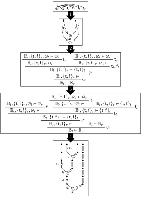
The ﬁrst way uses derivation trees in an ad hoc sequent calculus. We deﬁne a category T(A Ȃ B) whose objects are trees of conclusion (A Ȃ B) and whose morphisms are inclusions of such trees, and a subcategory B(A Ȃ B) of branches of conclusion (A Ȃ B). We decompose the desired square into

V_A,B B(A Ȃ B) EV(A Ȃ B)

P_A,B T(A Ȃ B) E(A Ȃ B)

iTO i

by ﬁrst showing that T(A Ȃ B) is equivalent to E(A Ȃ B), that this equivalence restricts to an equivalence between B(A Ȃ B) and EV_{(A Ȃ B), and then by}

building a full embedding from PA,B to T(A Ȃ B) and showing that it restricts

to an equivalence between VA,B and B(A Ȃ B). This is however not entirely

satisfactory in the sense that trees are not handled very formally, and a formal deﬁnition of T_{(A Ȃ B) would make the problem as diﬃcult to solve as without} using T(A Ȃ B).

We thus then give a formal construction of F and FV_{without using T}(A Ȃ

B). The proofs are much more ad hoc than in the rest of this thesis, which is not very surprising in the sense that we are trying to link models that are built using very diﬀerent methods.

(22)

1.3.3 A Core of Game Models

In Chapter 6, we want to build diﬀerent categories of strategies from a basic description of a game model. We start from some data P that describes a game model. For all games A, P gives a category PA of plays on the game A. It also

gives, for all games A and B, a category PA,B of plays on the pair(A, B), and

similarly for triples and quadruples of games. It also gives insertion functors, for example ι0∶ PA,B → PA,A,B that typically duplicates what happens on the

left-hand side game, and deletion functors, for example δ1∶ PA,B,C → PA,C that

typically erases what happens on the middle game.

We abstractly derive a notion of strategy from P: a strategy on the pair of games (A, B) is a presheaf over PA,B (we only study strategies on a pair of

games because we want to show that they form a category, but we could deﬁne strategies on a single game similarly). The idea is that a strategy σ accepts a play p if σ(p) ≠ Ȃ (more precisely, σ(p) is the set of states the strategy can be in after playing p). To show that games and strategies form a category, we then deﬁne a composition as parallel composition plus hiding and identities for this composition, known as copycat strategies.

The parallel composition σ∥τ of two strategies σ on (A, B) and τ on (B, C) accepts to play an interaction sequence (a play on three games) u if and only if σ accepts to play the projection δ2(u) of u to (A, B) and τ accepts to play

its projection δ0(u) to (B, C). The hiding of a strategy σ on PA,B,C accepts to

play p if and only if there is an interaction sequence u that projects to p that σ accepts to play, i.e., it accept the same plays as σ, except we hide what happens on B. Finally, the copycat strategy on the game A is a strategy on PA,Athat

“copies” all the moves Opponent plays.

In our framework, both composition and copycats are deﬁned as polynomial functors. Given a functor F∶ C → D, the restriction functor ∆F∶ D

Ȃ

→ CȂ

is given by pre-composition by Fop_{. It admits left and right adjoints}

∑F∶ C Ȃ → DȂ and ∏F∶ C Ȃ → DȂ

, called left and right Kan extension, respectively. The intuition behind_∑F is that the presheaf∑F(X) is non-empty over an element d if there

exists an antecedent c of d such that X is non-empty over c. For _∏F, the

intuition is that X must be non-empty over all antecedents of d. These functors can thus be seen as∃ and ∀ functors. A functor from CȂto DȂis polynomial if it is a composite of any number of restrictions and left and right Kan extensions.

Composition must be a functor from PA,B

Ȃ

× PB,C

Ȃ

to PA,C

Ȃ

. This is the same thing as a functor from PA,B+ PB,C

Ȃ

to PA,C

Ȃ

. We deﬁne it as the composite P_A,B+ P_B,C Ȃ∆_δ2+δ0 ÐÐÐÐ→ PA,B,C+ PA,B,C Ȃ∏_∇ ÐÐ→ PA,B,C Ȃ∑_δ1 ÐÐ→ PA,C Ȃ ,

where ∇ is the codiagonal functor. This is indeed a polynomial deﬁnition, and the idea behind it is exactly that of parallel composition plus hiding, which we can see by computing this functor, using the description of Kan extensions given above. The composite of the ﬁrst two functors is parallel composition: if it maps the copairing[σ, τ] to θ, then computation shows that θ accepts to play the interaction sequence u if and only if, for all antecedents u′_{of u (that is inl u}

and inr u),[σ, τ] accepts to play (δ2+ δ0)(u′), i.e., σ accepts to play δ2(u) and

τ accepts to play δ0(u). The last functor ∑δ1 is hiding: if it maps σ to τ , then

τ accepts to play p if and only if there exists an interaction sequence u that projects to p and is accepted by σ.

(23)

Copycat strategies are also deﬁned as polynomial functors. The copycat strategy on A may be deﬁned as a functor from 1 to PA,A

Ȃ . Since 1≅ ȂȂ , we can deﬁne it as: Ȃ Ȃ ∏! Ð→ PA Ȃ ∑_ι0 ÐÐ→ PA,A Ȃ .

The idea is that_∏!is the terminal presheaf on PA, so it accepts all plays in PA,

and_∑ι0(σ) accepts a play p if and only if p is of the form ι0(p

′_{) and σ accepts}

p′. Since ι0 typically corresponds to copying what happens on A to the other

copy of A, the whole composite indeed corresponds to the copycat strategy on A: it accepts to play p if and only if Proponent copies everything Opponent does.

We then set out to show that games and strategies form a category whose composition and identities we have just deﬁned. This means that composition must be associative and that the copycat strategies should be its units. We prove that, under some conditions, composition is associative and copycat strategies are units. The main condition is inspired by the method that is usually used in game models to show that composition of strategies is associative: the zipping lemma, which states that, in some cases, given two interaction sequences that project to the same play, there is a unique way to build a generalised interac-tion sequence (a play on four games) that projects to the original interacinterac-tion sequences.

All this work is done using our notion of concurrent strategy, and we want to get the same results for “traditional” strategies, which we see as functors Pop_A,B → 2, where 2 is the ordinal 0 → 1 seen as a category. We derive from the fact that games and concurrent strategies form a category that games and traditional strategies also do. We also investigate a number of game models and show that they ﬁt in this framework, and that composition of strategies in these game models corresponds to composition of strategies as deﬁned abstractly in our framework.

Finally, we tackle the question of innocence. We assume that we are given a full subcategory VA,B

iA,B

ÐÐ→ PA,Bof views to each category PA,B. We then deﬁne

innocent strategies as those presheaves that are in the image of VA,B

Ȃ ∏iA,B

ÐÐÐ→ PA,B

Ȃ

. The idea of this deﬁnition is that a presheaf_∏iA,B(σ) accepts to play p if

and only if, for all morphisms v→ p from a view v to p, σ accepts to play v. For this deﬁnition to be the right one, PA,Bshould contains enough morphisms (in

the case of HON games, the notion of morphism is that given by Melliès [80], reused by Levy [73] and Tsukada and Ong [96]). Such a presheaf thus accepts to play p if and only if it accepts to play all its views, which is the idea of innocence. We then set out to show that games and innocent strategies form a subcategory of games and strategies. By adding some properties on the model, we show that this indeed holds.

It may be interesting to see how we prove this kind of results. For example, let us take preservation of innocence, which states that the composite of two innocent strategies is again innocent. We prove this by studying the diagram below. (The reader does not need to understand this diagram.)

(24)

V_A,B+ V_B,C V_(A,B),(B,C) V_A,B,C V_A,C VA,B+ VB,C PA,B+ PB,C P(A,B),(B,C) PA,B,C PA,C

∏

∆ ∑

∏ ∏

∏ ∏ ∆ _∑

Notice that it does not make sense to ask whether this diagram commutes, since there is no starting or ending point in it. However, when it is lifted to categories of presheaves (where the ∆, _{∑, and ∏ labels show how to lift functors), all ∆} arrows are reversed, and the diagram turns into a diagram for which it makes sense to ask whether it commutes or not. When we lift this diagram to presheaf categories, the bottom row corresponds to taking two innocent strategies and composing them, so if the diagram (lifted to presheaf categories) commutes, then the composite of any strategies is in the image of_∏iA,C, and is thus innocent.

In the lifted diagram, the left-hand square commutes because the underlying one does, and the middle square commutes because the underlying one is exact. We thus only have to check that the right-hand one commutes, which is more diﬃcult. Basically all the proofs in this chapter follow a common pattern. We study the underlying diagram and

• for all squares that are made exclusively of ∆ (resp._{∏, resp. ∑), we show} that the square commutes,

• for all squares that are of the form A B C D ∏ ∆ ∆ ∏ A B C D ∑ ∆ ∆ ∑

we show that the square is exact, which entails that the lifted square commutes up to isomorphism,

• for squares of the form

A B C D

∑

∏ ∏

∑

(25)

Chapter 2

Preliminaries

In this chapter, we give a list of results from the state of the art that will be used in this dissertation. In this thesis, each section will be prefaced by a list of the preliminary sections that the reader should have read to understand the current section.

2.1 Game Semantics

We will be mostly interested in a particular version of game semantics, called arena games. The idea, in all these models, is to interpret types as arenas and programs as strategies on arenas of the right type. The definitions of these game models mostly follow the same pattern: they first define their notion of arena, which usually describe all the possible ways a program of a given type may perform a single reduction step, then plays, which describe a particular interaction between a program and an environment, and finally strategies, which usually consist of a set of accepted plays.

Being able to compose strategies is an important part of game semantics, since this is why game semantical models are compositional: the strategy as-sociated to the composite of two functions is the composite of the strategies associated to those functions. To define composition of strategies, all these models define interaction sequences, which basically represent the interaction of two plays. Finally, to show that composition of strategies is associative, they define generalised interaction sequences, which represent the interaction of three plays.

In Section 2.1.1, we study a game model called HON games. We then study a few possible variations of HON games, which are obtained by slightly changing the notion of play, in Section 2.1.2. Finally, we study Tsukada and Ong’s games, which are another variation of HON games, in which the notion of morphism is diﬀerent, in Section 2.1.3. In Section 2.1.4, we study AJM games, which are another game model. Finally, we study Blass games in Section 2.1.5, which are games that are well-known for their non-associative composition.

In Chapter 5, we will be interested in Tsukada and Ong’s games, and their links to string diagrammatic models. In Chapter 6, we will be interested in all the game models we describe in this section.

(26)

2.1.1 Hyland-Ong/Nickau Games

Required: Ȃ. Recommended: Ȃ.

For this model and a few others, the presentation we adopt is inspired by Harmer’s PhD thesis [46], because it unifies and simplifies many different frame-works.

Definition 2.1.1. An arena is a triple (A, λ, Ȃ) where A is a set, λ∶ A → {P, O} × {!, ?} is a function, and Ȃ ⊆ A × A is a relation that verifies:

• for all m in A, if there is no n such that nȂ m, then λ(m) = (O, ?), • for all n and m in A such that mȂ n, λOP_{(m) ≠ λ}OP_{(n), where λ}OP _is

defined as π1λ,

• for all n and m in A such that mȂ n, if λ?!(n) = !, then λ?!(m) = ?, where

λ?! _{is defined as π} 2λ.

Terminology 2.1.2. In an arena(A, λ, Ȃ), the elements of A are called moves, λis called the labelling function, andȂ is called the enabling relation. A move m is said to enable a move m′ if mȂ m′. The set of all moves of A will be denoted by MA, or sometimes simply A.

A move is initial (and is called a root of A) if there is no move that enables it. The set of roots of A is denoted √A.

A move m is an Opponent move when λOP_{(m) = O, and a Proponent}

move otherwise. A move m is a question when λ?!(m) = ?, and an answer

otherwise. In these terms, the constraints verified by λ state that all roots of A are Opponent questions, that the enabling relation alternates between Opponent and Proponent, and that answers are always enabled by questions.

Remark. Most of the settings we will study use exactly the same notion of arena, and only differ from HON game semantics because they impose different constraints on plays. AJM games and Blass games use different notions of arenas. There is also one model based on HON games that uses a different notion of arena: Tsukada and Ong’s games, in which the enabling relation forms a forest.

Example 2.1.3. The boolean arena B comprises three moves: q, which is an Opponent question, and t and f, which are Proponent answers. It may be drawn as a graph:

q

t f,

where the arrow denotes the enabling relation. This representation may be aug-mented with annotations for questions and answers to fully represent B, but since we will not need to be very formal about arenas, except in the case of Tsu-kada and Ong, who do not use questions and answers, we decide not to write them for conciseness.

(27)

To model the interaction between a program fragment and its environment, game semantics uses sequences of moves in an arena. For example, the following sequence is an interaction between a program fragment computing a boolean, and its environment:

q t q f.

The ﬁrst move corresponds to the environment asking for the value of the boolean. The second one corresponds to the program fragment answering that question by telling the environment that the boolean is true. The third and fourth moves play the same roles as the two previous moves, except that the program fragment answers that the boolean is false. This program fragment could, for example, be incrementing a reference each time it is called upon and answer true or false depending on the parity of that reference.

Obviously, some sequences of moves do not make sense. For instance, an-swering the value of a boolean before the environment even asked for that value makes little sense. Interactions are therefore represented by justified sequences, which prohibit such patterns by requesting that all moves be “justiﬁed” by some previous move.

Definition 2.1.4. A justiﬁed sequence on an arena(A, λ, Ȃ) is a triple (n, f, ϕ) where n is a natural number, f is a map from n to A and ϕ is a map from n to {0} Ȃ n, such that, for all i ∈ n,

• ϕ(i) < i,

• if ϕ(i) = 0, then f(i) ∈√A, and • if ϕ(i) ≠ 0, then f(ϕ(i)) Ȃ f(i).

Justified sequences equipped with prefix ordering form a category PA.

Remark. The notation PA for justified sequences on A is non-standard.

Usu-ally, plays on an arena A are defined like what we call plays on a pair of arenas in this dissertation (see below). We however prefer this definition because:

• it allows us to consider projections PA,B→ PA and PA,B→ PB, which is

impossible with the traditional notion of play on A,

• but it does not influence our study of strategies, since we only consider strategies built on PA,B’s (see below) and not PA’s.

Terminology 2.1.5. In a justified sequence (n, f, ϕ), if ϕ(i) = j, we say that j justifies i, or that j is the justifier of i. The arrow that points from i to j is called a justification pointer.

Justified sequences will be drawn as sequences of moves, to be read from left to right, with arrows pointing from each move to its justifier, as is classic in game semantics.

Our example above can thus be redrawn with justiﬁcation pointers as: q t q f.

Game semantical frameworks then go on to define what a play is. A play represents a particular type of interaction between a function and an environ-ment. In order to define them, we first need to define arenas for function types, which we do now.

(28)

To represent the interaction of a function of type A→ B and its environment, we build an arrow arena AȂ B from the arenas A and B.

Definition 2.1.6. The arena AȂ B is defined by • MAȂB= MA+ MB,

• λ_AȂB= [λA, λB], where λ is (s×{?, !})λ, where s is the swap function on

{O, P},

• and, for all m and m′ in MAȂB, m ȂAȂB m′ if and only if any of the

following holds:

– mȂAm′ or mȂBm′, or

– m is in√B and m′is in √A.

If we draw arenas as trees, then we may draw AȂ B as: B

A

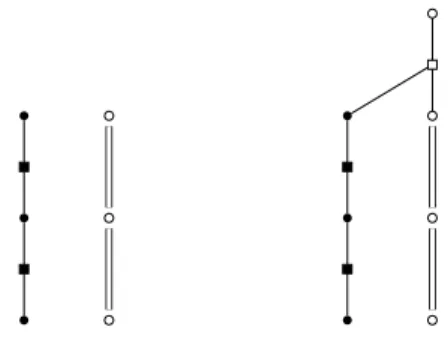
In other words, A Ȃ B comprises the moves from A and those from B, with exactly the same structure, except that initial moves in A are enabled by initial moves in B and that polarity is reversed in A. An interaction in such an arena is thought of as a player who may play on two games: as Proponent in B and as Opponent in A (this is rendered explicit by the fact that polarity is reversed in A). To easily tell in which part of AȂ B a move is played, we draw such interactions as a sequence of moves to be read from top to bottom, with the moves of A played on the left and those of B played on the right, as in:

B B qr

ql

tl

fr.

In this interaction, a player plays on two boolean games, one on the left and one on the right. They play as Proponent on the right-hand side game and as Opponent on the left-hand side one. For simplicity let us call this player M (for “middle”). There are two other players L and R who play Proponent on the left-hand game and Opponent on the right-hand game, respectively (they may also be thought of as a single player that represents the whole environment).

The drawing above represents a possible interaction of the not function on booleans with an environment.

• The ﬁrst move of the interaction (qr), which is played by the environment

(represented by the player R on the right), corresponds to asking the function to compute its result.

(29)

• In order to compute that result, the function must know the value of its argument. It thus asks the value of that argument to its environment, and more precisely to another program fragment that is represented by the player L on the left, by playing ql.

• After computing the value of that boolean, L answers the value of the boolean: the boolean is true, which is encoded in the fact that L plays tl.

• Since M now knows the value of its argument, it can ﬁnally answer what its result is by playing fr.

This example illustrates why there should be a change of polarity in A: when the function asks for the value of its argument, it plays the role of the environment to the program fragment that computes this argument, thus it should be playing as Opponent on A.

We may also sometimes write plays on arenas A_{Ȃ B like other plays, in} which case we will write ml or mAif the move m is played in the left-hand side

arena and mr or mB if it is played in the right-hand side one.

Now that we have defined arenas for functional types, we may come back to the definition of plays. The exact notion of play differs between frameworks, but they all amount to imposing constraints on justified sequences. We will use the following notion of play in this manuscript, as well as numerous variations on it, which we will describe later.

Definition 2.1.7. A play on the pair of arenas (A, B) is a justified sequence (n, f, ϕ) on A Ȃ B that is:

• alternating: for all i< n, λOP_{(f(i)) ≠ λ}OP_{(f(i + 1)),}

• of even length: n is even.

Prefix ordering between plays is defined in the obvious way: (n, f, ϕ) is a prefix of (m, g, ψ) if and only if n ≤ m and, for all i ≤ n, f(i) = g(i) and ϕ(i) = ψ(i). Plays on the arena pair(A, B) equipped with prefix ordering form a category PA,B.

In the other variants of game semantics discussed below, the notion of play is modified by adding further constraints on them. In the case of Tsukada and Ong’s model, however, there is a more fundamental difference between the categories of plays: their categories of plays have more morphisms than those simply given by prefix ordering.

A program fragment is then interpreted as a set of plays. The intuition is that a program fragment is interpreted as the set of interactions it can actually have with an environment. Such a set of plays is called a strategy.

Definition 2.1.8. A strategy on the arena pair(A, B) is a prefix-closed set of plays on(A, B).

Sometimes, strategies are also asked to be non-empty (i.e., to contain at least the empty play). A strategy σ is said to accept the play s if s∈ σ and to reject it otherwise.

Preﬁx-closedness comes from the fact that, if a program and its environment may interact, then they can have exactly the same interaction, but cut at some point, so if a strategy accepts a play, it should also accept all its preﬁxes.

(30)

Example 2.1.9. Let us consider the not function on booleans. It may be in-terpreted as a strategy on the arena BȂ B that accepts all plays s = (2n, f, ϕ) such that, for all i in n:

• if f(2i − 1) = qB, then{ f(2i) = qA

ϕ(2i) = 2i − 1 , • if f(2i−1) = tA, then{ f(2i) = fB

ϕ(2i) = ϕ(2i − 1) − 1 , and similarly if f(2i−1) = fA.

This illustrates the behaviour of the not function:

• whenever the environment asks for the value of not on a boolean (when there is a qB move), the strategy asks for its argument (by playing qA) and

remembers which question it is trying to answer, which is represented by the justification pointer pointing to a qB,

• whenever it receives a value for its argument (either tA or fA), it answers

the environment’s corresponding qB question with the right value (either

fB or tB); to know which qB question it should answer, the strategy looks

at which of its qA question was answered (by looking at the justification

pointer of the tA or fA move) and answers the corresponding qB question,

which necessarily comes just before the qA question.

A nice feature of game semantics is that it may interpret different classes of functions depending on the restraints imposed on strategies. For example, the strategy in the example above is very constrained, in the sense that Proponent may not do much: the move it plays only depends on the previous move and its justification pointer. In other words, its reaction only depends on the current “call to the function”. Technically, this strategy is innocent (this term will be defined later). Such strategies may only interpret purely functional programs.

Here is an example of strategy that is not innocent:

Example 2.1.10. Let us consider a boolean function that keeps a reference to an integer, increments it each time it is called, and returns either its argument if the reference is even, or its negation if the reference is odd. This function is not purely functional, since it modifies the value of a reference. The strategy associated to such a function could, for example, be the strategy σ that accepts all plays s= (n, f, ϕ) such that, for all i ∈ n:

• if f(2i − 1) = qB, then{ f(2i) = qA

ϕ(2i) = 2i − 1 ,

• if f(2i − 1) = bA and the number of qB moves in s∣2i−1 is odd, then

{ f(2i) = not bB

ϕ(2i) = ϕ(2i − 1) − 1 , and similarly when the number of qB moves is even, with f(2i) = bB.

This strategy indeed has the expected behaviour, since it answers either as the notfunction or as the identity, depending on how many times it has been called (given by the number of qB moves). Notice how this strategy no longer depends

only on the current call to the function, but also on how many times the function has been called in total (this means that the strategy is not innocent).

Categories and String Diagrams for Game Semantics

HAL Id: tel-02147264

https://tel.archives-ouvertes.fr/tel-02147264

Submitted on 4 Jun 2019

HAL is a multi-disciplinary open access

archive for the deposit and dissemination of

sci-entific research documents, whether they are

pub-lished or not. The documents may come from

teaching and research institutions in France or

L’archive ouverte pluridisciplinaire HAL, est

destinée au dépôt et à la diffusion de documents

scientifiques de niveau recherche, publiés ou non,

émanant des établissements d’enseignement et de

recherche français ou étrangers, des laboratoires

Categories and String Diagrams for Game Semantics

Clovis Eberhart

To cite this version:

Clovis Eberhart. Categories and String Diagrams for Game Semantics. Computer Science and Game

Theory [cs.GT]. Université Grenoble Alpes, 2018. English. �NNT : 2018GREAM091�. �tel-02147264�

THÈSE

Pour

obtenir le grade de

DOCTEUR

DE

LA COMMUNAUTÉ UNIVERSITÉ

GRENOBLE

ALPES

Spécialité

: Mathématiques

Clovis

Eberhart

Thèse

dirigée par Tom Hirschowitz

préparée

au sein du Laboratoire de mathématiques

et

de l’Ecole Doctorale de Mathématiques, Sciences et Technologies

de

l’Information, Informatique

Catégories

et diagrammes de

cordes

pour les jeux concurrents

Categories

and String Diagrams for

Concurrent

Game Semantics

Thèse

soutenue publiquement le 22 juin 2018,

devant

le jury composé de :

Mr.

Martin Hyland

M.

Samuel Mimram

M.

Pierre-Louis Curien

M.

Vincent Danos

M.

Paul-André Melliès

M.

Tom Hirschowitz

Thanks

Contents

Chapter 1

Introduction

1.1

Semantics of Programming Languages

1.1.1

An (Outdated) Map of Semantics

1.1.2

Semantics Today

1.2

Game Semantics

1.2.1

The Birth of Game Semantics

1.2.2

The Rich World of Game Models

1.3

_DE

_Eberhart

_{et diagrammes de}

_{pour les jeux concurrents}

_{and String Diagrams for}

_{Game Semantics}

_{soutenue publiquement le 22 juin 2018,}