HAL Id: halshs-00175010
https://halshs.archives-ouvertes.fr/halshs-00175010
Submitted on 26 Sep 2007
HAL is a multi-disciplinary open access archive for the deposit and dissemination of sci-entific research documents, whether they are pub-lished or not. The documents may come from teaching and research institutions in France or abroad, or from public or private research centers.
L’archive ouverte pluridisciplinaire HAL, est destinée au dépôt et à la diffusion de documents scientifiques de niveau recherche, publiés ou non, émanant des établissements d’enseignement et de recherche français ou étrangers, des laboratoires publics ou privés.
Theories
David Dickinson, Marie Claire Villeval
To cite this version:
David Dickinson, Marie Claire Villeval. Does Monitoring Decrease Work Effort? The Complementar-ity Between Agency and Crowding-Out Theories. 2004. �halshs-00175010�
Does Monitoring Decrease Work Effort?
The Complementarity Between Agency
and Crowding-Out Theories
David Dickinson Marie-Claire Villeval
DISCUSSION P
APER SERIES
Forschungsinstitut zur Zukunft der Arbeit Institute for the Study of Labor
Does Monitoring Decrease Work Effort?
The Complementarity Between Agency
and Crowding-Out Theories
David Dickinson
Appalachian State University
Marie-Claire Villeval
GATE, CNRS,
University of Lyon 2 and IZA Bonn
Discussion Paper No. 1222
July 2004
IZA P.O. Box 7240 53072 Bonn Germany Phone: +49-228-3894-0 Fax: +49-228-3894-180 Email: iza@iza.orgAny opinions expressed here are those of the author(s) and not those of the institute. Research disseminated by IZA may include views on policy, but the institute itself takes no institutional policy positions.
The Institute for the Study of Labor (IZA) in Bonn is a local and virtual international research center and a place of communication between science, politics and business. IZA is an independent nonprofit company supported by Deutsche Post World Net. The center is associated with the University of Bonn and offers a stimulating research environment through its research networks, research support, and visitors and doctoral programs. IZA engages in (i) original and internationally competitive research in all fields of labor economics, (ii) development of policy concepts, and (iii) dissemination of research results and concepts to the interested public.
IZA Discussion Papers often represent preliminary work and are circulated to encourage discussion. Citation of such a paper should account for its provisional character. A revised version may be available on the IZA website (www.iza.org) or directly from the author.
ABSTRACT
Does Monitoring Decrease Work Effort?
The Complementarity Between Agency
and Crowding-Out Theories
Agency theory assumes that tighter monitoring by the principal should motivate the agent to raise his effort level whereas the “crowding-out” literature suggests that it may reduce the overall work effort. These two assertions are not necessarily contradictory provided that the nature of the employment relationship is taken into account (Frey, 1993). Based upon a real-task laboratory experiment, our results show that principals are not trustful enough to refrain from monitoring the agents, and most of the agents react to the disciplining effect of monitoring. However we find also some evidence that intrinsic motivation is crowded out when monitoring is above a certain threshold. We identify that both interpersonal principal/agent links and concerns for the distribution of output payoff are important for the emergence of this crowding out effect.
JEL Classification: M5, J24, C92
Keywords: principal-agent theory, monitoring, crowding-out, motivation, real effort experiment
Corresponding author: Marie-Claire Villeval GATE
93, chemin des Mouilles 69130 Ecully
France
consider the absence of agent monitoring by a principal as a weakness that can be exploited by rational cheaters because of the disutility of effort. However, little monitoring may also be considered an expression of trust that can be rewarded through effort. As a consequence, additional monitoring of agent performance should diminish shirking (i.e., increase worker effort) in one case, whereas in the second case monitoring should diminish effort by focusing on the market exchange nature of the employment relationship and by reducing intrinsic motivation for effort. These different rationales are grounded in two opposing theories. On the one hand, based on self-interested behavior, agency theory assumes that tighter monitoring by the principal should motivate the agent to raise his effort level in order to reduce the risk of a penalty if caught shirking (Alchian and Demsetz, 1972; Calvo and Wellisz, 1978; Fama and Jensen, 1983; Laffont and Martimort, 2002; Prendergast, 1999). On the other hand, the “crowding-out” theory1 suggests that tighter monitoring may reduce overall work effort
because of the hidden cost of sanctions. According to this theory, economic incentives such as monetary rewards or sanctions may undermine intrinsic motivation if they are considered as being controlling, thus reducing either the agents’ esteem or
1 The crowding-out theory has been mostly developed by social psychologists in connection with the
so-called cognitive evaluation theory (Deci, 1971, 1975; Deci, Koestner and Ryan, 1999). These analyses have notably emphasized the hidden cost of rewards (Lepper and Greene, 1978). The existence of a crowding-out effect of intrinsic motivation is, however contested (Prendergast, 1999) or neglected by most economists. Exceptions are Titmuss, 1970 (who argued that paying for blood donation would destroy the willingness to donate) and more recently, Bohnet, Frey and Huck, 2000; Drago, 1989; Frey, 1997; Frey and Oberholzer-Gee, 1997; Gneezy and Rustichini, 2000; Kreps, 1997, Benabou and Tirole, 2002. In particular, Kreps states that if employees develop intrinsic motivation in reaction to fuzzy extrinsic incentives, the introduction of explicit incentives may diminish intrinsic motivation for work. Benabou and Tirole try to reconcile psychology and economic approaches showing that rewards may be strong, weak or negative reinforcers depending on the ability of the agent, the attraction and its discussion of the task, the asymmetry of information regarding the agent’s talent and the nature of the task.
determination.2 Monitoring is thus considered as signal for lack or breach of trust. This
interpretation is also consistent with the social exchange theory (Blau, 1964; Hollander, 1990; Homans, 1961).
In this paper, we test experimentally these two opposing assertions considering that they are not necessarily contradictory provided that the nature of the principal-agent relationship is taken into account. Frey, 1993 distinguishes the disciplining effect and the crowding-out effect of monitoring and hypothesizes that the disciplining effect will likely dominate in abstract relationships, while the crowding-out effect is likely to dominate in interpersonal relationships. In the latter case, more monitoring may be interpreted by the agent as a sign of distrust that will crowd-out intrinsic motivation and lead to lower effort. In contrast, in an abstract relationship, no such psychological effect should arise because there are no personal trust or benevolence relationships between the principal and the agent. The aim of our study is thus to use a controlled real-task laboratory experiment to analyze the influence of the nature of the employment relationship on the relative importance of disciplining effect and the crowding-out effect of monitoring on the agents’ work effort.
Psychologists have provided compelling experimental evidence for the existence of a crowding-out of intrinsic motivation by rewards (see the meta-analysis by Deci, et al., 1999, and its critics by Eisenberger, Pierce and Cameron, 1999). Experimental economists have also recently collected evidence on this effect (Fehr and Gächter, 2002; Frey and Jegen, 2000; Gneezy and Rustichini, 2000; Gächter and Falk, 2002).3
2 Corroborating this analysis, Bewley, 1999 shows, from interviews with managers and labor leaders, that
the risk for managers of using threats is a loss of worker initiative.
3 Gneezy and Rustichini (2000) show that the subjects working for free reached the same level of
performance that the subjects who received a high pay and a much higher outcome than those who were paid a small amount of money. Fehr and Gächter (2002) and Gächter and Falk (2002) provide
However, evidence of a crowding-out effect of the probability of monitoring instead of
certain rewards on performance remains scarce and the lack of naturally-occurring data
usually leads to indirect tests of competing hypotheses. Some supporting evidence for the crowding out hypothesis is found in a survey of managers, where Barkema, 1995, and Frey, 1993 document a negative effect of monitoring on hours worked when the principal is a CEO but a positive effect when the manager is supervised impersonally by a parent company. Nevertheless, the data is not conclusive given the measurements used and the difficulty in controlling for confounding factors.4 An experimental
procedure can help mitigate such concerns by collecting controlled data on both monitoring and performance.
Other evidence is found in more controlled settings. A field experiment on call centers confirms the rational cheater hypothesis but shows that employees do not respond to the exogenous manipulation of monitoring rates when they think the employer is being fair (Nagin, Rebitzer, Sanders and Taylor, 2002). In a laboratory experiment, Schulze and Frank, 2003 show that monitoring reduces corruption through deterrence but it also destroys the intrinsic motivation for honesty. With ultimatum games, Guerra, 2002 observes that by reducing trust opportunities, monitoring has a negative impact on the behavior of honest individuals. Indirect evidence is also provided by Fehr and Schmidt, 2000, who show that effort is lower when principals condition a fine on the deviation from the desired effort level. Finally, Fehr and List, 2002 observe both hidden costs of sanctions (the use of an explicit threat to sanction shirking backfires by inducing less
experimental evidence that incentive contracts are less efficient than contracts without any incentives because of the crowding-out effect; nevertheless principals prefer using the incentive contracts because they can reach a higher share of the surplus.
4 Managers’ effort is measured by the number of hours worked and the intensity of monitoring by the
regularity, the specificity and the formality of the evaluation procedure. However, there is no direct connection between the content of the evaluation procedure and the level of work effort supplied.
trustworthy behavior) and hidden rewards (refraining from using an available threat is considered a trusting act reciprocated by a trustworthy choice of effort).
Our approach contributes to the existing literature on discipline vs. crowding-out effect of monitoring in three ways: it uses a real task experiment; it analyzes whether these effects depend on the nature of the employment relationship; it studies whether they differ according to the sharing rules of the output between the principal and the agent (i.e., the payoff rules). The principal determines her intensity of monitoring by choosing among audit or monitoring probabilities ranging from no monitoring (0%) to certain monitoring (100%). This intervention may be considered as controlling and not informative. Informed of this probability, the agent has to perform a costly real task. Choosing a value of effort from a table of hypothetical effort cost choices, as in some of the existing research, may involve intrinsic motivation like reciprocity. However, we prefer a real effort experiment because it also involves intrinsic motivation for the task itself and is more parallel to a real work setting. Thus, our paper also contributes to the experimental literature analyzing effort in a real work setting (Falk and Ichino, 2003; Dickinson, 1999; Sillamaa, 1999; van Dijk, Sonnemans and van Winden, 2001; Gneezy, Niederle and Rustichini, 2003; Montmarquette, Rulliere, Villeval and Zeiliger, 2005). To measure the influence of the nature of the employment relationship, the experiment was conducted in two environments. An “abstract employment relationship” is proxied by using a stranger matching protocol so that no principal engages in a repeated interaction with the same employee. Our proxy for an “interpersonal relationship” is a partner matching protocol in which decision-making is no longer anonymous. In addition, under the partner matching that we utilize, the subjects of the same principal/agent pair are given time to introduce themselves to each other before
engaging in the experimental decision-making. Because the members of the pair know that they will be able to comment on their respective decision at the end of the session, the absence of anonymity introduces an informal control which, according to the crowding-out theory, should both reduce the intensity of monitoring and increase its crowding-out effect.
To identify the influence of distributional concerns, we compare two treatments. In one treatment, the principal’s payoff increases in the agent’s effort (the Variable treatment) whereas in the other one, the principal’s payoff is not directly affected by agent effort (the Fixed treatment). Fehr and Rockenbach, 2003 hypothesize that the negative motivational effects of sanctions on altruistic cooperation appear if associated with greedy or selfish intentions. This suggests that in the Fixed treatment monitoring should not be interpreted as motivated by greediness or selfishness but by the willingness to enforce the respect of a non-shirking norm; one should then only observe the disciplining effect of monitoring. Thus, we have a 2x2 experimental design (abstract/interpersonal and Fixed/Variable).
Our results indicate that the disciplining effect of monitoring dominates in abstract relationships as expected but is also present in interpersonal relationships. Whatever the nature of the relationship, principals are not trustful enough to refrain from monitoring and most agents react to the disciplining effect of monitoring by increasing effort. However, we also observe some evidence of a crowding-effect of intrinsic motivation when some specific conditions are met. An indication of the existence of intrinsic motivation lies in the fact that a significant proportion of the agents perform at the desired output level when their principal shows no willingness to monitor. Monitoring may undermine intrinsic motivation when the monitoring intensity exceeds its
equilibrium level, when the employment relationship is based on interpersonal links and when distributional concerns are at work.
The reminder of the paper is organized as follows. Section 2 presents the structure and the different treatments of the monitoring game, and its theoretical predictions. Section 3 introduces the experimental design. Section 4 presents the statistical analysis and its results. The final section discusses and concludes.
2. The monitoring game
The game involves two players, a principal and one agent, i ∈
{
P A,}
. An output , y, is produced by the agent. This output depends on the agent’s effort and on the difficulty of his task. From this basic structure, we examine two treatments which differ in the effect of this output on the payoffs of the principal. In the Variable Treatment, additional effort by the agent directly increases the payoff of the principal. Alternatively, in the Fixed Treatment, the agent’s effort does not directly affect the principal’s payoff. After a description of these Treatments, theoretical predictions will be drawn.2.1.Two Treatments
Consider first the Variable Treatment. In Stage one, the principal offers the contract
(
W w w y y m to the agent, consisting of three wage levels, W, w and, , , , ,ˆ)
w ,corresponding to various levels of outputs, a desired level of output ˆy , a minimum
output requirement y , and a probability of audit m (i.e., the monitoring intensity).
Payment to the agent is W =100 if his output is not audited or if it meets the desired level of output ˆ 75y= in the event of an audit. If audited and output is between the
minimum, y=40, and the desired level (i.e., y≤ yi < ) then w=60 is paid. Finally, if yˆ the output is below the minimum requirement yi < , then the agent receives the y
minimum wage w=20. The monitoring intensity, m∈
(
.0,.1,...,1)
, represents the probability that the agent’s output will be audited, and it is the only decision variable for the principal. Monitoring is costly for the principal beyond some minimum level,0.2
m= . The intuition is that below a certain level, monitoring is not costly because simple observation may be sometimes sufficient to detect shirking. If shirking at some level has been verified, the principal punishes him by paying a lower wage, w or w . The differences between W and w and between W and w can be considered as fines, and the size of the fine depends on the extent of shirking.
The principal chooses her intensity of monitoring according to its cost, given by the following convex cost function:
( ) (
1.5m m)
2c m
b
−
= (1)
with m= , the threshold for a free monitoring and .2 b=.02.
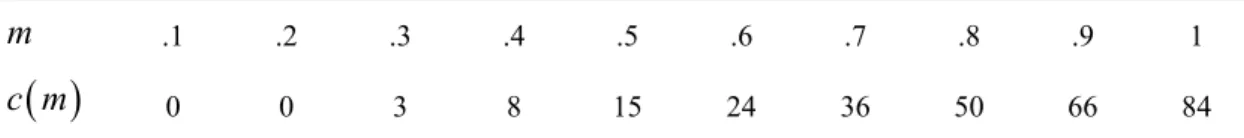
After rounding numbers up, monitoring costs are displayed in Table 1.
Table 1. Monitoring costs by intensity of monitoring
m .1 .2 .3 .4 .5 .6 .7 .8 .9 1
( )
c m 0 0 3 8 15 24 36 50 66 84
The (expected) payoff function of the principal in the Variable Treatment is given by: (2)
( )
(
) ( )
(
) ( )
ˆ ˆ i i PV i i i i vy W c m if y y vy W m W w c m if y y y vy W m W w c m if y y π − − ≥ = − + − − ≤ < − + − − < with v=2.5 (each unit of output of the agent increases the principal’s payoff by 2.5). In Stage two, once the principal chooses a contract
(
W w w y y m , the agent is then , , , , ,ˆ)
informed of this contract and cannot reject it.5 Knowing his payoff function, the payofffunction of the principal, and the monitoring probability, the agent has to decide on his level of effort needed to produce the output yi∈
(
0,1,...,100)
.The agent has to perform a real task, inspired from Montmarquette, et al., 2005 and described in detail below. This task consists of progressing along a curve and output is measured by the height reached on this curve. Progression on the curve is made by means of regular-steps that are free and by means of rapid-steps that are costly. Performing a higher output usually entails a marginally increasing monetary cost that is linked to speed of progression chosen by the agent:
( )
i ( r r)c y = f α s (3)
where s is the number of rapid-steps and α the cost of these steps, and the subscript r
indicates the rank of these costly steps. c
( )
0 =0 and c y( )
= , that is, the minimum 0 required output can always be performed without any monetary cost. In the experiment, the convexity of costs is given as follows:Table 2. Costs of the rapid steps
Rank of the rapid-steps 1 to 10 11 to 20 21 and more
Cost of each rapid-step .4 .6 1.0
5There is no stage in the game where the agent accepts or rejects the contracts. The experiment is setup so that the participation and incentive compatible constraints are always met from the beginning. A subject who would like to express negative reciprocity must do it through his effort decision.
Ten different curves are used in the experiment and they are designed such that, on average, it costs 20 points to perform ˆy (this information is common knowledge). The minimum cost is 0 and the maximum cost is 70 depending on the difficulty of the curves. W ≥c y
( )
* ensures that the participation constraint holds.The agent’s (expected) payoff function is given by:
( )
( )
(
)
( )
(
)
ˆ ˆ i i i i i i i W c y if y y W c y m W w if y y y W c y m W w if y y π − ≥ = − − − ≤ ≤ − − − < (4)Once the agent has performed the task, in Stage three, the monitoring probability is applied, the audit occurs or not depending on the draw, and payoffs are displayed. Consider now the Fixed Treatment. The principal also offers the contract
(
W w w y y m to the agent with the same wage values and corresponding output , , , , ,ˆ)
thresholds, the same monitoring cost function than in the Variable Treatment. But in contrast, the principal’s payoff consists of a flat fee and no longer increases in the agent’s output. The principal’s (expected) payoff function in the Fixed Treatment is now given by:
(5)
where f =180 is the flat fee given to the principal. The agent has the same payoff and cost functions as in the Variable treatment.
( )
( )
(
) ( )
ˆ ˆ ( ) i PF i i f W c m if y y f W m W w c m if y y y f W m W w c m if y y π − − ≥ = − + − − ≤ < − + − − < 2.2.Theoretical Predictions
Consider first the Variable Treatment and the behavior of the agent. A risk-neutral and selfish agent performs at the desired output level ˆy if his certain payoff of no shirking is equal or higher than the expected benefit of producing an output below the desired level ˆy and below the minimum required output y . Considering that wages are flat fees (either equal to W, w or w ), the agent should not choose any other output than y or 0, once he has decided to shirk. So, we have two no-shirking conditions depending on the reference level of output, ˆy or y :
No-shirking condition 1:
(
ˆ)
( )ˆ(
)
[
( )]
(
1)
( )
i yi y W c y E i yi y m w c yi m W c yi π ≥ = − ≥ π < = − + − − (6) No-shirking condition 2:(
ˆ)
( )ˆ(
ˆ)
[
( )]
(
1)
( )
i yi y W c y E i y yi y m w c yi m W c yi π ≥ = − ≥ π ≤ < = − + − − (7)Since c y
( )
=c( )
0 = , the binding constraint (7) for reaching ˆy simplifies as: 0c y
( )
ˆ ≤m W w(
−)
(8) That is, the marginal cost of ˆy must be less than or equal to its marginal benefit.In addition, a rational and selfish agent should never perform more than ˆy with costly steps since performing more than ˆy yields no additional earnings to the agent. The best reply output choices *
i
y for a selfish agent to each monitoring intensity depends on the
comparison between expected marginal cost and expected marginal benefit of choosing ˆy vs. y . With our parameterization and an average cost of 20 necessary to reach the desired output level, the best reply effort changes at m=.5. Below this level, the
marginal cost of ˆy exceeds its marginal benefit so that the agent should choose zero
effort in response to the absence of monitoring and y for any positive value of m. The optimal output of a rational and selfish agent in the Variable Treatment is thus:
0 0 * .5 ˆ .5 iV if m y y if m y if m = = < ≥ (9)
An incentive compatible contract leads to * ˆ
iV
y = for any monitoring probability at y
least equal to .5.
Consider now the decision of a profit-maximizing principal. The principal chooses the monitoring intensity that maximizes her expected payoff considering the rational choice of the agent. This maximization can be written as:
( )
( )
(
1)
[
( )]
V PV V i V V i V
m
Max Eπ =m vy % −c m −w%+ −m vy% −c m −W (10)
i
y% is the expected output from agent i and w% is the expected wage depending on the verified level of output. With probability m , output is audited and W, V w or w is paid to an agent caught shirking. With probability
(
1−mV)
, output is not verified and Wis paid. The monitoring cost appears in both terms: the principal has to pay this cost whether shirking is detected or not.In equilibrium, mV should be chosen such that the marginal cost of monitoring equals
the expected marginal return of monitoring in terms of penalty (i.e., extra profit) for the principal if shirking is caught and in terms of additional output (increased monitoring may stimulate effort). Since both the choice of output and the monitoring intensity are discrete choices, we can only consider the numerical solution of the game. With our
parameterization, the principal reaches her maximum expected payoff when choosing .5
V
m = . Thus, in equilibrium, one obtains: * * .5 ˆ 75 100 20 80 187 15 100 72 V iV iV PV m y y π π = = = = − = = − − =
Consider now the theoretical predictions for the Fixed Treatment. Regarding the agent’s decision, the same no-shirking conditions applies than in the other treatment:
( )
ˆ(
)
c y ≤m W w− . Optimal output is thus:
0 0 * .5 ˆ .5 iF if m y y if m y if m = = < ≥ (11)
The principal chooses the monitoring intensity that maximizes her expected payoff considering the rational choice of the agent. This maximization can be written as:
( )
( )
(
1)
[
( )]
F PF F F F F
m
Max Eπ =m f c m− −w%+ −m f c m− −W (12) with w% the expected wage depending on the verified level of output.
With our parameterization, the principal reaches her maximum expected payoff when choosing .3mF = . Thus, in equilibrium, one obtains:
* * 40 .3 (0.3)*60 (0.7)*100 88 (0.3)*(180 3 60) (0.7)*(180 3 100) 89 iF F iF PF y y m E E π π = = = = + = = − − + − − =
A selfish principal chooses a low probability of monitoring (.3). This contract is not efficient in the sense that the agent performs less than yi=75 in equilibrium. The agent
should stop his effort as soon as he reaches y , which he can always reach without bearing any monetary cost. Compared to the Variable Treatment, we should thus observe in the experiment a lower monitoring intensity and a lower output.
However, the above predictions to not consider any behavioral motivations, which may change these predictions for both treatments. A trustful principal could choose mV = . 0 A principal that does not use a costless opportunity to monitor signals her trust to the agent and the agent might be willing to reciprocate by increasing his effort. A principal who chooses a higher level of monitoring than .4 pushes the agent to perform the output of 75; in the fixed treatment, this can be understood as the principal’s willingness to enforce a non-shirking moral norm since it reduces her own expected payoff and is not rational from a strictly monetary point of view. An intrinsically motivated agent could perform at the desired output level even though he knows that the probability of being caught shirking is low or even absent either because he is motivated by the task or because he is willing to reciprocate the principal’s for her trust toward the agent. If the agent performs an output higher than 40 with a monitoring probability lower than .5, it may also indicate intrinsic motivation. Additionally, one can assume that these behavioral considerations are likely to be sensitive to the nature of the employment relationship and the payoff rules for the principal and the agent.
3. Experimental Design
We first focus on the originality of the experiment, regarding the design of the task to be performed by the agent and the design of the employment relationship. Then, the experimental procedures will be detailed.
3.1. Design of the task
The task of the principal-subjects is designed in a traditional way thatallows to control for the amount of resources devoted to tracking the effort of agents. The principal’s decision consists of choosing the monitoring intensity by means of a scrollbar on the computer screen. The choice of monitoring intensity is represented as a probability of audit choice on the agent’s performance by the computer program, including all deciles between 0 (no monitoring) and 1 (certain monitoring). The choice of probability 0 can be interpreted as a signal of trust to the agent since, below probability .3, monitoring is free of costs for the principal.
The design of the agent’s task is more original due to the real task requested from the subjects. Compared to the choice of effort values in tables, a real task experiment is closer to a real work setting and is more likely to involve intrinsic motivation for the task itself. Our experiment uses about the same design of the task as the one described in Montmarquette, et al., 2005, but in an individual work environment. The task consists of the search of the highest value of a multiple-peaked function in a two-dimension space defined vertically by height (H) and horizontally by distance (D) from the origin, with H∈
[
0,100]
and D∈[
0,300]
, with HMax = f D( )
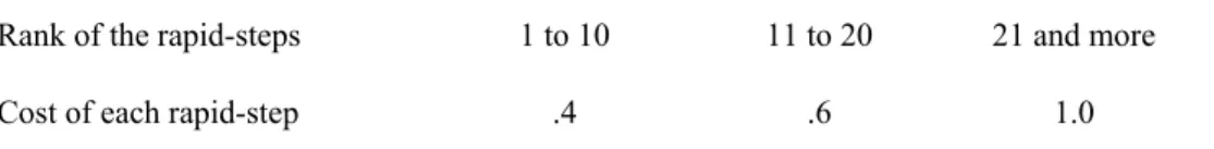
. The curvecorresponding to this function is increasing, with a maximum of three peaks. When the period starts, the box in which the curve will appear is fully black. During a one minute period, the agent-subject uncovers progressively the curve on his computer screen starting at the origin, by clicking a button. The subject moves by discrete steps on the horizontal axis that make him go upwards. The curve and its surface become visible as the subject progresses. The output achieved by the subject in a period is given by the
height reached on the curve, which depends notably on the number of moves. The subject can stop his progression whenever he wants by stopping clicking.
While performance is measured by the height parameter between 0 and 100, the cost of effort is captured through a monetary cost parameter. Cost is represented through the choice of the speed of progression. Parameters are chosen so that it is impossible to reach the required height during the one-minute period allowed by using the regular speed only. Two buttons are available: regular (“1-steps”) or fast (“2-steps”), the second option enabling a twice as rapid move as the first option. The subject can switch speeds whenever he wants and without any restriction in frequency. The regular speed is costless, whereas each step is costly as indicated in Table 2: each of the first 10 2-steps costs .4 point; each of the 10 further 2-2-steps costs .6 and each further 2-step costs 1 point. On average, reaching the height 75 costs 20 points and this is common knowledge.
Figure 1. An example of the task to be performed
Each new period is associated with a new randomly chosen curve.6 As soon as a new
period starts, the subject’s computer screen indicates currently the time left, the
6 The set of curves used in this experiment can be found at the following address:
cumulated cost of 2-steps, and the height reached (see Fig.1). These curves represent various degrees of difficulty depending on both the horizontal distances between the 75-height and the origin and between the maximum 75-height and the 75-75-height. An index of difficulty is calculated as 10 D
(
75+(
D100−D75)
)
, with D the abscissa at the origin of 75the 75-height and D the abscissa of the maximum height. 100
The cognitive dimension of this task relates to the uncertainty about the shape of the curve, to time pressure and to the subject’s decision to use the fast speed. For example, without any ex ante information about the shape of the curve, if a subject has already used many rapid moves to hasten progression and the curve remains flat, paying each additional costly step requires a continuous trade-off between its marginal cost and its expected marginal revenue. At every point on the curve, the subject can never infer from the already uncovered part of the curve the slope of this curve at the next points. As a consequence, the task has a cognitive component since the subject cannot discover one single algorithm and he must make a continuous trade-off between his speed and the time left. This is an important difference with other real effort experiments, notably van Dijk et al. (2001). In addition, the design of this task leaves no room for a fear of dismissal, the search for co-workers’ esteem, or the disapproval of pairs who can be considered in natural settings as fuzzy motivators misattributed to intrinsic motivation (Kreps, 1997).
3.2. Design of the employment relationship
Frey, 1993 states that the disciplining effect of monitoring should be associated with an abstract employment relationship whereas its crowding-out effect would be associated with an inter-personal relationship. In order to assess both effects, we utilize two
distinct experimental protocols to proxy abstract versus interpersonal relationships between principal and agent. To identify the behavioral effect of these procedures, all the subjects were submitted to both protocols. Specifically, a stranger matching protocol is used to proxy an abstract employment relationship with no repeated interactions. With this protocol, principals and agents are randomly re-matched after each period and this is common knowledge.
To proxy an interpersonal relationship, we allow for social exchange and social approval by using a partner matching protocol and by lifting anonymity of the subjects interacting in the same pair. Specifically, a principal-agent pair is randomly matched and remains paired for ten periods, and subjects are made aware of this. In addition, the subjects of each matching pair are introduced to each other. The two members of each pair are seated face-to-face and they are given five minutes to talk together for introducing themselves to each other. The subjects are aware that they are not allowed to comment on the experiment and on their past or their future decisions and they are not allowed to pass any side-payment agreement or to threat their partner. This is controlled by the circulation of the experimentalists in the lab who could have kept the subjects to the rules if it had been needed. To facilitate this introduction process and to focus the discussions on personal issues, we distributed a questionnaire sheet to each pair of subjects.7 This sheet of paper consisted of two parts, one about each member of
the pair. Each principal was requested to ask the questions to her agent and to write his answer, and vice-versa for the agent. This moment was quite popular in all the sessions and it created a very animated and courteous atmosphere. At the end of this introduction process, the members of a pair remain seated side by side but no longer
7 This questionnaire included questions about their given name, their number of siblings, their favorite
face-to-face and they are not allowed to communicate any more. This proximity is, however, such that each subject can anticipate that at the end of the session the members of the pair will be able to discuss and comment on their respective decisions.
The aim of this design with repeated interactions that lifts anonymity is to emphasize the importance of social exchange and social approval considering that it constitutes a key aspect of interpersonal relationships (Blau, 1964). This design has no implications on the theoretical predictions of the game with selfish preferences of the subjects. It may have behavioral consequences by narrowing the social distance and by favoring empathy between the principal and the agent. Research in online communication has also shown that, when comparing forms of communication like text-chat, text-to-speech and voice in social dilemma games, voice results in the highest level of cooperation (Jensen, Farnham, Drucker and Kollock, 2000). The impact of personal identification in experiments has been documented by various studies (see Kachelmeyer and Shebata, 1997 for public goods games, Sally, 1995 for social dilemmas, and Falk et al, 1999 for the gift-exchange game).
3.3 Experimental procedures
Ten 20-period sessions of this experiment were realized in the experimental laboratory of GATE (Groupe d’Analyse et de Théorie Economique), Lyon, France. Five sessions implemented the Variable Treatment and five other sessions the Fixed Treatment. In total, we obtained 920 observations with the Variable Treatment and 900 with the Fixed Treatment. In each slot of sessions, three out of five sessions implemented first the stranger matching protocol and then the partner protocol, the two other sessions
implemented the reverse order.8 This gives a total of 910 observations in each
environment. 182 student-subjects were drawn from the undergraduate classes of the Chemicals and Textile School, the School of Management, the Central School of Engineers and a minority of students came from the department of economics. No subject participated in more than one session.
On average, a session lasted 75 minutes including initial instructions, practice periods and payment. The experiment was computerized using the REGATE program (Zeiliger, 2000). Transactions were conducted in Experimental Currency Units, with the ECU-Euro conversion rate set at ECU 150 = € 1. The final payoff was given by the sum of the earnings in each period. In addition, a show-up fee consisted of two elements. First, at the beginning of the session and before the presentation of the instructions, each subject had to choose between two options consisting of either participating in a lottery with an expected payoff of € 2.5 or taking a certain gain of € 2, at the end of the session. This gives an (imperfect) indication about the subjects’ risk aversion that can be controlled for in the regressions to explain individual behavior. Second, at the beginning of the game, each subject received an initial endowment of 150 ECUS to deal with the possibility of a loss in the first period. On average, each subject earned € 13.42 (S.D.=2.65).9 Subjects were immediately paid in cash in a separate room.
Participants were randomly assigned to a specific computer terminal, depending on the computer name drawn randomly from an envelope upon entering the room. Written
8 8 sessions were initially realized in which the order of the curves was the same in both parts of the
experiment. 2 additional control sessions (one for each treatment) were conducted in which the order of the curves was changed in the second part of a session to control for a possible memory effect. A mean test shows that the average effort is not significantly different according to the order of the curves in the second part at the 5% level.
9 With an average of € 13.35 for the principal-subjects (S.D.=2.87) and € 13.48 for the agent-subjects
instructions were distributed to participants and read aloud by the experimenter (see Appendix). All participants were thus completely informed about the rules and parameters of the game. Instructions were phrased in neutral terms.10 Questions were
answered privately by the experimenter. Two practice periods were run11 and a
questionnaire was passed to check the understanding of the instructions by the subjects before the first part of the experiment began. Each subject was then randomly assigned by the computer the role of either principal (“X subject”) or agent (“Y subject”). Each participant kept the same role throughout the session. At the end of the first part, the game stopped and further instructions for the second part were distributed, without any questions allowed.
At the beginning of each period, the X-subject chooses [0.0,0.1,0.2,0.3,0.4,0.5,0.6,0.7,0.8,0.9,1.0]
m∈ . The Y-subject was informed of this
probability and had then to perform his task, deciding on his cost of effort. At the end of the one-minute period of time, his output is checked according to the probability level chosen by the principal. Then payoffs are displayed and a new period starts automatically. At the end of each period, both the principal and the agent receive feedback on the output realized, whether audit occurred, and their actual payoffs.
4. Experimental results
We consider first the summary statistics before analyzing the principal and agent behaviors by means of a panel data analysis.
10 We spoke about a curve, an outcome, a check, a payoff, and we avoided loaded terms such as effort,
monitoring and wage.
11 Each subject had to practice the task to be performed by the sole agents afterwards because at this stage
the subjects are not aware yet of the role they will be assigned and because it makes the principal aware of the possible difficulty of the task.
4.1. Summary statistics
The data collected by means of this real-task experiment help in testing three main predictions of the model and its behavioral extensions. The first two predictions relate to the principals’ decisions and the third one to the agents’ activity.
First, under the assumption of selfishness, the monitoring probability is expected to be greater than .3 on average and should not be affected by the nature of the employment relationship. In contrast, if the principal anticipates an agent’s intrinsic motivation in the experiment, then this should lead her to lower her monitoring intensity or even to give up monitoring, at least in the interpersonal employment relationship.
We observe that the average monitoring probability is .369 in the abstract employment relationship and .361 in the interpersonal employment relationship. The difference is not significant according to a Wilcoxon signed-rank test (z = .357).12 There is no
monitoring in only 3.51% of the observations in the interpersonal relationship and 2.31% in the abstract employment relationship; the difference is not significant (Wilcoxon test, z = -1.436). This suggests that the principals do not fully trust their agents even though they are engaged in an interpersonal relationship. Intrinsic motivation, if it exists, is not thought to be sufficient to motivate the agent to perform the requested output level.
Second, under the assumption of selfishness, the monitoring intensity should be higher in the Variable Treatment than in the Fixed Treatment. If the monitoring intensity in the Fixed Treatment is equal or higher than in the Variable one, it is consistent with a willingness to enforce a moral norm.
12 In all the Wilcoxon tests which results are reported in this section, we consider 10 independent
observations consisting of each of the 10 sessions. One session cannot give more than one independent observation because of the reshuffling of the pairs of subjects at each repetition of the game in 10 periods out of 20 when the stranger matching protocol is in use.
The observed average monitoring probability is .386 in the Variable Treatment and .344 in the Fixed Treatment. The monitoring probability is slightly lower than the equilibrium value in the Variable Treatment (.5) and slightly higher in the Fixed Treatment (.3). A Mann-Whitney test indicates that the probabilities are significantly different at the 5% level (z = -1.984). However, this test is not very robust since we have only 5 perfectly independent observations in each treatment (one per session). Most principals choose to not reduce their payoffs—by increasing the monitoring probability beyond its equilibrium level—to enforce a moral norm.
Third, under the assumption of selfishness, the level of output performed by the agents should increase in the monitoring intensity due to its disciplining effect, whatever the treatment and the nature of the employment relationship. However, if the agent is intrinsically motivated, the level of output should be indifferent to the monitoring intensity. If monitoring crowds out intrinsic motivation, the level of output is likely to be inversely related to the monitoring intensity, at least in the interpersonal relationship. A variant of the latter hypothesis is that the level of output should be higher when the principal does not exert her monitoring power in an interpersonal relationship because the agent can reciprocate to the trust signaled by the principal.
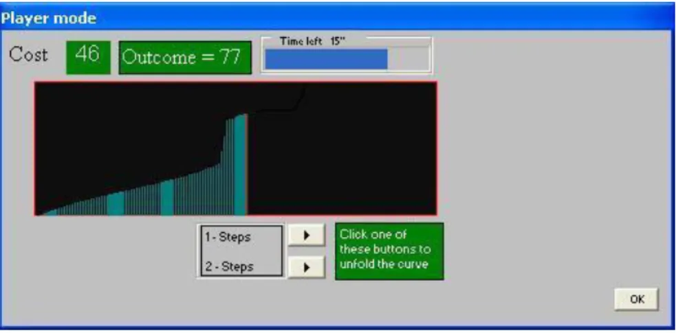
Figure 2. Distribution of the shares of output by monitoring intensity 0,00 10,00 20,00 30,00 40,00 50,00 60,00 70,00
ProbMonit=0 0<ProbMonit<.4 ProbMonit>=.4
<40 40 to 74 75 and +
Figure 2 shows that the share of an output at least equal to the desired level of 75 clearly increases in the monitoring intensity. This tends to support the rational cheater hypothesis and the disciplining effect of monitoring. Intrinsic motivation is not strong enough to guarantee the realization of the desired output in any monitoring circumstances. Strong shirking (an effort level below 40) reacts to the introduction of a monitoring probability (its share decreases from 18% to 4%) but not to its intensity. However, some subjects still supply effort even when there is no risk of sanction— about a quarter of the agents perform at the desired output level or even above this level when m=0. In addition, near a third of the agents do the same when the monitoring probability is in between .1 and .3, even though they should not produce y>40 in (selfish) equilibrium. This may indicate that a fraction of the agents experience some level of intrinsic motivation, either for the interest of the task, for the principal’s choice not to monitor or to monitor below the equilibrium, or by integrity and commitment to moral principles.13
We made the behavioral hypothesis that the relationship between output and monitoring is related to the nature of the relationship between the principal and the agent. Surprisingly, the average output is 69.53 in the abstract relationship and 70.07 in the interpersonal relationship. The difference is not significant (Wilcoxon test, z = -0.255). The picture is somewhat more complicated when we relate average output to the monitoring intensity.
13 From an extensive U.S. survey about worker motivations, Minkler, 2004 shows that the rank-order of
motivations is moral duty, intrinsic motivation, peer pressure and incentives. To a question about their motivation if it is impossible for their employer to check up of them, 83% of the respondents answered that they were “very likely” to work hard, and 12% that they were “somewhat likely” to do so. Our data reveal a smaller proportion but we directly measure the work output and not only declarations of intention.
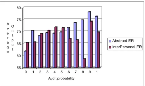
Figure 3. Average output by monitoring intensity and by type of employment relationship
Figure 3 displays the average output by monitoring intensity and by type of employment relationship. In an abstract employment relationship, the average effort increases relatively regularly with the audit probability, emphasizing the disciplining effect of monitoring. In an interpersonal employment relationship, the average output is higher than in the abstract environment for most monitoring probabilities up to .5, and especially at m=0. However these differences are not significant (Wilcoxon test, z = -1.274). In contrast, beyond this probability, the average output becomes systematically lower than in the abstract relationship; this difference is only significant at the 14% level (Wilcoxon test, z = 1.478). Agent output declines in the monitoring intensity, except when monitoring becomes certain or quasi-certain. This cannot be explained by a lower risk aversion of the subjects (the Spearman coefficient of the correlation between risk aversion and effort is not significant; ρ=.11). In such an environment, the disciplining effect of monitoring might be partly counteracted by its crowding-out effect. 55 60 65 70 75 80 A v e r a g e O u t p u t 0 .1 .2 .3 .4 .5 .6 .7 .8 .9 1 Audit probability Abstract ER InterPersonal ER
The relationship between the principal and the agent also depends on the output sharing, or payoff, rule. Despite a significantly weaker monitoring intensity in the Fixed Treatment, the average output is higher in this treatment (71.06) than in the Variable Treatment (68.57) and this difference is significant at the 5% level (Mann-Whitney test, z = 1.984). This tends to indicate that effort is not only influenced by an intrinsic motivation for performing the task, risk aversion, individual monetary rewards, and the nature of the employment relationship, but also by distributive considerations, as already largely documented by inequality aversion theories (see Bolton and Ockenfels, 2000; Fehr and Schmidt, 1999). A figure displaying the average output by monitoring intensity and by type of treatment (not reported here) shows the same characteristics as Figure 3. In the Fixed Treatment, the average output increases regularly in the monitoring intensity whereas in the Variable Treatment, it declines beyond a monitoring probability of .4, except when auditing is certain or quasi-certain. In the Fixed Treatment, the intrinsic motivation for the task does not seem to be altered and the agents react to the disciplining effect of the increased monitoring intensity. Since in this treatment the principal receives a fixed payoff, increasing her cost of monitoring is likely associated with the enforcement of a norm and this does not entail any negative reaction from the agent. In contrast, in the Variable Treatment, reducing his output is a costly way for the agent to punish the principal for choosing a high monitoring intensity. This is costly to the agent since it increases his risk of being caught shirking and it represents a sanction for the principal since her payoff is directly linked to the output level. Thus, when distributional concerns are at work, increasing the monitoring intensity tends to undermine intrinsic motivation.
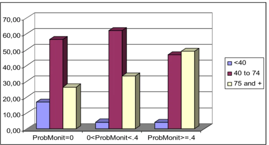
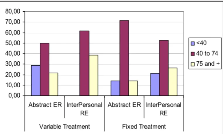
Figure 4. Distribution of the shares of output by type of employment relationship and by treatment when the principal chooses not to monitor
Figure 4 only refers to those cases in which the principal chooses not to monitor the agent. It shows that the difference in the proportion of strongly shirking agents between an abstract employment relationship and an interpersonal one is larger in the Variable than in the Fixed Treatment. Since, in the Variable Treatment the principal’s payoff increases in the agent’s output, giving up the monitoring opportunity is a stronger signal of trust than in the Fixed Treatment. Positive reciprocity may explain that in this case no agent engaged in an interpersonal relationship fully shirks, and near 40% of them perform at the desired level (instead of 26.3% in the Fixed Treatment), although it is costly for the agent and it only increases the principal’s payoff.
However, one must be cautious about these indications since the number of observations in which the principal chooses m=0 is low (53 out of 1820 total observations). More generally, these non parametric statistics are based on a small number of independent observations. In addition, summary statistics do not control for time, difficulty of the curves and individual effects. Regression analyses controlling for
0,00 10,00 20,00 30,00 40,00 50,00 60,00 70,00 80,00 Abstract ER InterPersonal RE Abstract ER InterPersonal RE Variable Treatment Fixed Treatment
<40 40 to 74 75 and +
these dimensions are needed to identify the determinants of two endogenous variables at the individual level: monitoring intensity and output levels.
4.2. Statistical analysis
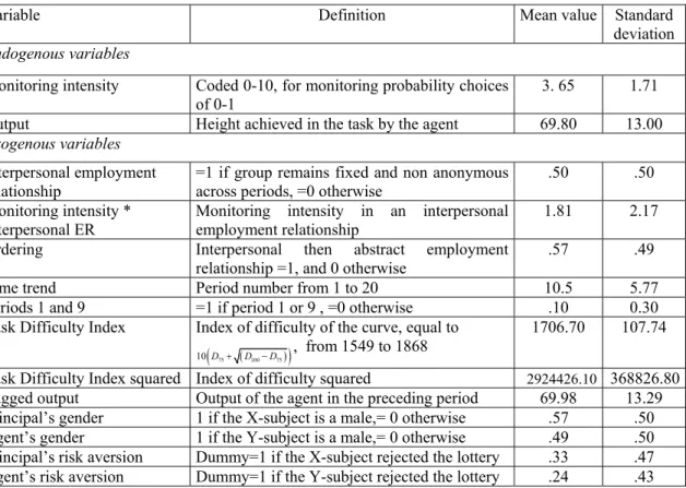
Table 3 presents the definition and descriptive statistics of variables used in the regressions to explain the endogenous variables, monitoring intensity and output level.
Table 3. Variables and descriptive statistics
Variable Definition Mean value Standard
deviation Endogenous variables
Monitoring intensity Coded 0-10, for monitoring probability choices
of 0-1 3. 65 1.71
Output Height achieved in the task by the agent 69.80 13.00 Exogenous variables
Interpersonal employment
relationship =1 if group remains fixed and non anonymous across periods, =0 otherwise .50 .50 Monitoring intensity *
Interpersonal ER
Monitoring intensity in an interpersonal employment relationship
1.81 2.17 Ordering Interpersonal then abstract employment
relationship =1, and 0 otherwise .57 .49 Time trend Period number from 1 to 20 10.5 5.77
Periods 1 and 9 =1 if period 1 or 9 , =0 otherwise .10 0.30 Task Difficulty Index Index of difficulty of the curve, equal to
( )
( 75 100 75)
10 D + D −D , from 1549 to 1868
1706.70 107.74
Task Difficulty Index squared Index of difficulty squared 2924426.10 368826.80 Lagged output Output of the agent in the preceding period 69.98 13.29 Principal’s gender 1 if the X-subject is a male,= 0 otherwise .57 .50 Agent’s gender 1 if the Y-subject is a male,= 0 otherwise .49 .50 Principal’s risk aversion Dummy=1 if the X-subject rejected the lottery .33 .47 Agent’s risk aversion Dummy=1 if the Y-subject rejected the lottery .24 .43
The exogenous variables are: the nature of the employment relationship, the environment ordering (when an interpersonal relationship precedes an anonymous one), a time trend, an index of difficulty for each curve and an index of difficulty squared. The lagged output level is also taken into account in the regressions to check how the principal reacts to the agent’s behavior. An interaction term between the type of the employment relationship and the monitoring intensity is also entered in the regressions. Lastly, demographic variables such as gender are entered to control for their potential
impact. Since variables such as school or age, the ordering of employment relationships, and the lagged audit and sanctions turned out not to be significant, they are omitted from the regressions presented below.
We use random-effect GLS models to accommodate the data and explore first the determinants of the choice of a monitoring intensity by the principals (see Table 4) then the determinants of the output levels reached by the agents (see Table 5). We consider the Variable and the Fixed Treatments in separate regressions.
Table 4. The determinants of the monitoring intensity
Dependent variable:
Monitoring intensity Random effects GLS model
Treatment Variable Fixed
Interpersonal employment relationship
Lagged output
Time trend
Principal’s risk aversion
Principal’s gender Constant - .065 (.475) - .020*** (.000) .035*** (.000) .128 (.680) .586** (.043) 4.532*** (.000) .014 (.898) - .015*** (.002) - .052*** (.000) .444* (.102) .300 (.251) 4.735*** (.000) Nb of observations Wald χ2 Prob > χ2 Overall R2 828 62.39 0.000 0.0816 810 44.37 0.000 0.0572
Note: The regressions have been realized with StataTM 8.0. p-values are in parentheses. *, **, ***
indicate statistical significance at the .10, .05, and .01 level, respectively.
In the regression reported in Table 4, we observe that, whatever the treatment and the type of the employment relationship, most principals use their monitoring power. They adjust their monitoring intensity to the output realized by the agent in the preceding
period even in an abstract relationship. This effect occurs in both Variable and Fixed Treatments. Thus, the fact that the principals’ payoffs could be affected by the agents’ output is not a determining factor of this effect. In addition, there is no evidence that the repeated-interaction nature of the interpersonal employment relationship has any additional effect on principals’ behavior.
Another significant effect of interest is the coefficient on the time trend variable. The results indicate a trend over time of more monitoring in the Variable Treatment but less monitoring over time in the Fixed Treatment, ceteris paribus. This may be in response to the downward trend of agents’ effort over time in the Variable Treatment (see Table 5), which is of less direct importance to the principals in the Fixed Treatment. This shows clear indication that principals are responding to the agency theory incentives of monitoring when own-payoffs are directly at stake. Lastly, the principals’ risk aversion plays positively only in the Fixed Treatment whereas in the Variable Treatment, males are less trustful than females.
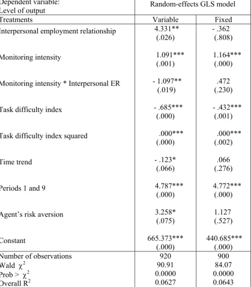
Table 5 shows results from our modeling of agents’ behavior. While the intensity of monitoring is not influenced by the type of the principal-agent relationship, output is significantly higher in an interpersonal employment relationship in the Variable Treatment. There is some evidence of a disciplining effect of monitoring as indicated by the positive and significant coefficient on the monitoring intensity variable in both treatments. But in the Variable Treatment, there is also an indication of a crowding-out effect of monitoring on output in the interpersonal employment relationship: output is negatively influenced by the intensity of monitoring when principals and agents interact repeatedly. The crowding-out effect is not visible in the Fixed Treatment, probably because there is no selfish intention attributed by the agents to the principals whose
payoffs do not increase in the level of output performed by the agents. It suggests that the crowding-out effect of monitoring on effort is related to distributive considerations.
Table 5. The determinants of the agent’s output
Dependent variable:
Level of output Random-effects GLS model
Treatments Variable Fixed
Interpersonal employment relationship
Monitoring intensity
Monitoring intensity * Interpersonal ER
Task difficulty index
Task difficulty index squared
Time trend
Periods 1 and 9
Agent’s risk aversion
Constant 4.331** (.026) 1.091*** (.001) - 1.097** (.019) - .685*** (.000) .000*** (.000) - .123* (.066) 4.787*** (.000) 3.258* (.075) 665.373*** (.000) - .362 (.808) 1.164*** (.000) .472 (.230) - .432*** (.001) .000*** (.002) .066 (.276) 4.772*** (.000) 1.127 (.527) 440.685*** (.000) Number of observations Wald χ2 Prob > χ2 Overall R2 920 90.91 0.0000 0.0627 900 84.07 0.0000 0.0643
Note: The regressions have been realized with StataTM 8.0. p-values are in parentheses. *, **, ***
indicate statistical significance at the .10, .05, and .01 level, respectively.
Not surprisingly, the output level is also influenced by the degree of difficulty of the task in both treatments. Performance is lower when the profile of the curve makes reaching the desired target more costly. But this relationship is not linear. A possible explanation lies in the notion of job challenge, as already suggested in Montmarquette et al., 2005, and largely documented in the psychological literature (Locke, Saari, Shaw and Latham, 1981). A higher output is observed in the first and the ninth periods in
both treatments, probably due to learning and a restart effects, respectively. The coefficient on Time trend variable indicates that agents generally decrease their effort over time, ceteris paribus, though the effect is only significant in the Variable Treatment. In addition, in the Variable Treatment, risk aversion pushes the agents to increase their effort in order to avoid a possible sanction. In contrast, other specifications (not reported here) show that being audited or being sanctioned in the preceding period has no significant impact on the output realized in the current period. 5. Conclusion and discussion
The model provided by Frey, 1993 states that monitoring by a principal exerts a disciplining effect on agent’s effort in an abstract employment relationship whereas it has a crowding-out effect of intrinsic motivation when the principal and the agent are engaged in an interpersonal relationship because it reduces the scope for trust. Agency theory and crowding-out theory could thus be complementary provided that account is taken of the nature of the employment relationship. However, though the crowding-out effect of intrinsic motivation by monetary rewards has been largely documented in the literature, especially in psychology, empirical evidence of the crowding-out effect of monitoring has been scarce. Our real-task laboratory experiment aims at testing the complementarity of agency and crowding-out theories as regards the influence of monitoring on performance. We analyze the influences not only of the nature of the employment relationship but also of the sharing rules of the outcome, by comparing conditions where the employment relationship is either spot and anonymous or grounded in interpersonal links, and by comparing treatments in which the principal’s payoff increases or not in the level of agent’s performance.
Our main results show that both principals and agents respond to extrinsic incentives in the experimental design: (1) principals monitor less intensely when agents gave high effort in the previous period and monitoring trends up over time while agents’ output trends down, and (2) agents react to the disciplining power of the monitoring intensity by decreasing shirking when the perceived cost of such behavior is increased. A fraction of the agents are also guided by intrinsic motivation: (3) a relatively high proportion of agents perform at the desired output level also when principals trustfully give up their monitoring power. (4) Despite this observation, principals do not seem to believe in intrinsic motivation since they cannot refrain from monitoring their agents in most circumstances. The evidence in support of the crowding-out of intrinsic motivation is less clear. We observe that (5) when distributional concerns are at work (i.e. in the Variable Treatment) and when the employment relationship is based on interpersonal links, increasing the monitoring intensity beyond its equilibrium level tends to undermine intrinsic motivation. It shows that the disciplining effect and the crowding-out effect of monitoring may coexist in interpersonal relationships and that the crowding-out effect is probably associated with concerns for the distribution of payoffs between the principal and the agent.
These results tend to support the complementarity between agency theory and out theory. We do not find however systematic evidence of such a crowding-out effect. Several remarks could be done. First, our experimental design of the task to be performed by the subjects could be reproached for its insufficient ability to sustain intrinsic motivation. As remarked by Deci et al., 1999, if an activity is dull and boring, one cannot expect to find external events such as performance-contingent rewards that undermine intrinsic motivation. In our case, the task to perform was not a play task like
solving mazes or puzzles. But we can think that if it was considered too boring a task, we should have observed a systematic decrease of output over time in all treatments and conditions and in addition, we should not have ever observed any crowding-out effect. Second, the principal’s behavior with regards to monitoring is not affected by her being engaged in an interpersonal relationship. Again, our procedure for establishing a non-anonymous and repeated interaction could be criticized for its inability to reduce the social distance necessary for creating empathy and testing the crowding-out hypothesis. Experiments on rewards and intrinsic motivation in which anonymity was lifted and face-to-face procedures implemented have however shown that social pressure does not change significantly the slope of the wage-employment relationship compared to a standard repeated interaction (Falk, Gächter and Kovacs, 1999). If our procedure was inadequate in producing social approval/disapproval pressure, we should not observe any effect of this procedure on the agents’ behavior either, that is not the case. In fact, a study by Fehr and List, 2002, shows that even though the use of the threat to sanction shirking backfires by inducing less trustworthy behavior from the agents, the vast majority of subjects cannot refrain from using this threat. In our experiment, we observe comparable hidden costs of monitoring and hidden rewards of not using this opportunity: in the interpersonal relationship especially, the principals’ average earnings are higher in the absence of monitoring (92.59, S.D.=10.47) than when the principals choose the equilibrium value (74.82, S.D.=18.55) and than when they choose a monitoring probability greater than .5 (67.97, S.D.=21.56).
The social psychology of agency relationships has emphasized an extrinsic incentives bias, i.e. people think that the others are more motivated than themselves by extrinsic motivation and less motivated by intrinsic motivation (Heath, 1999). For economists,
the preference for monitoring despite its negative effect on monetary payoff remains a paradox. Our experiment suggests that this bias may exist; the average monitoring probability is greater in period 1 than in aggregate further periods although principals have no information on the motivation of their employees. It also suggests that the “excessive” use of monitoring by the principals (i.e. beyond its equilibrium level) as well as the reduction of effort by the agents beyond a certain monitoring threshold can be partly interpreted in terms of mutual punishment. Principals pay to use monitoring in order to punish agents who perform less than desired in the preceding period and agents reduce effort and thus decrease their own expected payoff in order to punish principals whose payoff is directly linked to the agents’ level of performance. As a consequence, it confirms that reducing monitoring activity in firms requires the prior establishment of mutual trust in order to be mutually beneficial.
Appendix. Instructions for the Variable Treatment (order: abstract relationship then interpersonal relationship)14
You are going to participate in an experiment which is part of a scientific program supported by the GATE research institute of the CNRS (National Center for Scientific Research), and by Utah State University in the U.S.A. During this experimental session, you are requested to make decisions and you can earn money. The amount of your earnings depends on your own decisions and on those of the other participants with whom you will interact.
This session consists in 2 parts of 10 periods each. The session should last about one hour. During this session, your payoffs will be calculated in ECU (Experimental Currency Units) and put on an account.
At the beginning of the session, your account will be credited of 150 ECUs, which are
given as an initial endowment.
During each period, you can earn or lose ECUs. Please note that your decisions can avoid
losses with certainty and that possible losses in some periods should be compensated for by earnings in other periods.
Your final earnings are equal to the sum of the ECU you will earn in each of the 20
periods. At the end of the session, the total amount of ECU you have earned on your account will be converted to Euros at the following rate:
150 ECU = 1 €
Your entire earnings in Euros will be paid in cash in a separate room to preserve confidentiality.
Throughout the entire session, talking is not allowed except when invited by the experimenter. Any violation of this rule will result in being excluded from the session and not receiving payment. If you have any questions regarding these instructions, please raise your hand. Someone will answer your questions privately.
During this session, the group of participants is subdivided into two categories in equal number: X and Y participants. Your computer indicates whether you are a X- or a Y-participant. Whether X or Y, you keep the same role throughout this session.
Rules for Periods 1-10
During each period, pairs of participants are randomly formed (each X-participant is matched with one Y-participant). At each new period, new pairs are randomly formed. You are not necessarily matched with the same person from one period to the other. Nobody will be informed of the identity of the participants s/he interacted with during these periods.
Roles
The X-participant asks the Y-participant to realize a task in exchange for which s/he will
receive a payment. S/He can apply a monitoring probability to Y’s result.
The Y-participant performs a task and achieves a result.
14 The other sets of instructions corresponding to the other treatments are available upon request to the