HAL Id: tel-01543080
https://tel.archives-ouvertes.fr/tel-01543080
Submitted on 20 Jun 2017HAL is a multi-disciplinary open access archive for the deposit and dissemination of sci-entific research documents, whether they are pub-lished or not. The documents may come from teaching and research institutions in France or abroad, or from public or private research centers.
L’archive ouverte pluridisciplinaire HAL, est destinée au dépôt et à la diffusion de documents scientifiques de niveau recherche, publiés ou non, émanant des établissements d’enseignement et de recherche français ou étrangers, des laboratoires publics ou privés.
Sensor Networks lifetime
Yousif Elhadi Elsideeg Ahmed
To cite this version:
Yousif Elhadi Elsideeg Ahmed. Modeling, Scheduling and Optimization of Wireless Sensor Networks lifetime. Performance [cs.PF]. Université de Lorraine, 2016. English. �NNT : 2016LORR0315�. �tel-01543080�
AVERTISSEMENT
Ce document est le fruit d'un long travail approuvé par le jury de
soutenance et mis à disposition de l'ensemble de la
communauté universitaire élargie.
Il est soumis à la propriété intellectuelle de l'auteur. Ceci
implique une obligation de citation et de référencement lors de
l’utilisation de ce document.
D'autre part, toute contrefaçon, plagiat, reproduction illicite
encourt une poursuite pénale.
Contact : [email protected]
LIENS
Code de la Propriété Intellectuelle. articles L 122. 4
Code de la Propriété Intellectuelle. articles L 335.2- L 335.10
http://www.cfcopies.com/V2/leg/leg_droi.php
Optimization of Wireless Sensor
Networks lifetime
by
Yousif Elhadi Elsideeg Ahmed
Submitted to the IAEM Lorraine Doctoral School in fulfillment of the requirements for the degree of
Doctorate
in
Automation, Signal and Image Processing, Computer Engineering
Dissertation Committee Imed KACEM Feng CHU Mhand HIFI Marie-Ange MANIER Zineb SIMEU-ABAZI Magdi B. M. AMIEN Kondo H. ADJALLAH Sharief F. BABIKIR
Prof. Universit´e de Lorraine Prof. U. d’Evry Val d’Essonne Prof. U. de Picardie Jules Verne MDC HDR U. de Technologie de Belfort-Montb´eliard
MDC HDR Grenoble Universit´e
Associate prof. U. of Gezira Prof. Universit´e de Lorraine Prof. U. of Gezira President Rapporteur Rapporteur Rapporteur Examiner Examiner Supervisor Co-supervisor
December 2016
Wireless Sensor Networks lifetime
Yousif Elhadi Elsideeg Ahmed
Abstract
Wireless sensor networks (WSNs), as a collection of sensing nodes with limited pro-cessing, limited energy reserve and radio communication capabilities, are widely implemented in many areas of applications such as industry, environment, health-care, etc. Regarding this large range of applications, many research issues are introduced including the applications, performance, reliability, lifetime, etc. The WSNs lifetime considered in this work is the period of time through which the WSN is perfectly completing its function. This lifetime is affected by many fac-tors including the amount of energy available, failure probability and components degradation. The amount of energy available become the most important factor in case of non renewable components applications. Different algorithms, strategies and optimization techniques were developed and implemented for this purpose based on the possibility of activating a subset of sensors that satisfied the moni-toring constraint, while keeping the others in sleep mode to be implemented later. This is an NP complete maximization problem that can be solved using disjoint set covers (DSCs). But the solution obtained using DSCs does not extend always significantly the WSNs lifetime. So, the present work aims to search for a better solution using non-disjoint set covers (NDSCs). This approach gives the oppor-tunity for a sensor to be implemented in one or more subset covers. For that purpose, we studied a binary representation based model to maximize the number of NDSCs. Also, we developed a genetic algorithm based heuristic based on this model to find out the maximum number of NDSCs in a reasonable time. Thus, for a set of m sensors used to monitor a set of n targets or a field, this heuristic allows to construct a maximum number q of NDSCs. Additional effort is required to find the best scheduling for implementing the NDSCs so as to maximize the lifetime of the sensors involved in the WSNs, considering their limited available energy. This problem is formulated using integer linear programming (ILP) mathematical model. The objective function of this problem is the sum of all monitoring seasons on which all q NDSCs scheduled, and the constraint is the energy consumption in
all sensors included in all NDSCs. Solving this problem using ILP in a period of time depends on the complexity of the model and the instances used. To find the solution in reasonable time, we have developed a NDSCs based genetic algorithm (NDSC-GA). The candidate solutions are represented in chromosomes composed of a number of genes equal to the number q of NDSCs, and each gene is the number of monitoring seasons on which a NDSC is scheduled. We have then developed a GA that combines the four crossover operators and four mutation operators. The GA based methods are coded in C programming language to obtain a satisfying solution and the Cplex software was used to obtain the corresponding exact solu-tion. Comparing the optimal solution obtained using the ILP on small instances, to the solutions obtained using our GA based method explained that our methods can find a solution near the optimal in reasonable time. Then, comparing the solution obtained using our NDSCs GA based methods, to the DSCs GA based method in the literature, we showed that the NDSCs GA can prolong the WSNs lifetime better than DSCs GA for the same instances. Our approach combines together the scheduling principles and the optimization techniques to maximizing the WSNs lifetime.
de la Dur´
ee de Vie des R´
eseaux de Capteurs
Sans Fil
Resum´
e
Les r´eseaux de capteurs sans fil (RCSFs), sont compos´es d’un ensemble de nœuds avec des capteurs, transmetteur/r´ecepteur, d’un syst`eme de traitement es d’un r´eserve d’´energie. Au regard d’applications, de travaux de recherche sont d´evelopp´es sur l’utilisation de ce r´eseau leur performance, fiabilit´e ou dur´ee de vie. La dur´ee de vie RCSFs correspond `a la p´eriode `a travers laquelle le RCSF fonctionne par-faitement. Cette dur´ee de vie est tr`es affect´ee par de nombreux facteurs comme la quantit´e d’´energie disponible, la probabilit´e de d´efaillance et les d´egradations des composants. L’´energie disponible devient le facteur pr´epond´erant dans les cas d’applications avec des composants difficilement rechargeables ou non renou-velables. Diff´erents algorithmes, strat´egies et techniques d’optimisation ont ´et´e ´
elabor´ees et mises en œuvre `a cet effet sur la possibilit´e d’activer un sous-ensemble de capteurs qui satisfont `a la contrainte de surveillance et de garder les autres capteurs en mode veille pour pouvoir ˆetre mis en œuvre ult´erieurement. Ainsi, c’est un probl`eme de type NP complet de maximisation qui peut ˆetre r´esolu en
consid´erant des Ensembles Disjoints de capteurs de Couverture (EDC). Mais la
solution obtenue `a l’aide des EDCs ne conduit pas toujours `a une extension sig-nificative de la dur´ee de vie des RCSFs. Le pr´esent travail vise `a rechercher une meilleure solution bas´ee sur des capteurs regroup´es dans des ensembles
non-disjointes de couverture (ECND). Cette approche permet `a un capteur de
par-ticiper `a une ou plusieurs ensembles de capteurs de couvertures. Nous avons alors ´
etudi´e un mod`ele de repr´esentation binaire des ECNDs pour d´eterminer un ordon-nancement optimum permettant de maximiser la vie d’un RCSF. De plus, nous avons d´evelopp´e une heuristique bas´ee sur un algorithme g´en´etique, pour
trou-ver une solution proche de l’optimal dans un d´elai raisonnable. Ainsi, pour un
ensemble de m capteurs utilis´es pour surveiller un ensemble de n cibles, cette
heuristique permet construire un nombre maximum q d’ensembles ECNDs. Des efforts suppl´ementaires sont donc n´ecessaires pour trouver le meilleur
ordonnance-ment pour la mise en oeuvre des ECNDs, qui maximise la dur´ee de vie globale
du RCSF, compte tenu de l’´energie initialement disponible dans chaque capteur. Ce probl`eme est formul´e `a l’aide d’un mod`ele math´ematique de programmation lin´eaire en nombres entiers (PLE). La fonction objective de ce probl`eme est la
somme de toutes les p´eriodes de surveillance pour les q ECNDs programm´es, et
la contrainte est la consommation d’´energie de tous les capteurs constituant les ECNDs. La possibilit´e de trouver la solution `a ce probl`eme par PLE dans une p´eriode de temps donn´ee d´epend de la complexit´e du mod`ele et des instances utilis´ees. Pour trouver la solution dans un d´elai raisonnable, nous avons d´evelopp´e un algorithme g´en´etique (AG) bas´e sur les ECNDs. Les solutions potentielles sont repr´esent´ees dans des chromosomes compos´es d’un certain nombre de g`enes corre-spondant aux ECNDs, et chaque g`ene est caract´eris´e par la p´eriode de surveillance d’un ECND. Nous avons ensuite d´evelopp´e un AG qui combine quatre op´erateurs de croisement et quatre op´erateurs de mutation. La m´ethode bas´ee cet AG a ´et´e cod´ee dans le langage de programmation C pour obtenir une solution satisfaisante et le logiciel Cplex a ´et´e utilis´e de d´eterminer la solution exacte correspondant. Une comparaison des solutions obtenues sur de petites instances en utilisant la
PLE par rapport aux solutions obtenues par notre AG montre que la m´ethode
bas´ee sur les AG peut trouver une solution proche de l’optimale dans un d´elai raisonnable. Ensuite, en comparant les solutions en utilisant l’AG ECNDs `a l’AG
EDCs de la litt´erature, nous montrons que l’AG avec ECND peut prolonger la
dur´ee de vie des RCSFs plus que les AG avec EDCs pour les mˆemes instances.
Notre approche combine ainsi les principes d’ordonnancement et les techniques d’optimisation pour maximiser la dur´ee de vie des RCSFs.
It is my great pleasure to express my sincere and deep thanks and gratitude to my supervisors Prof. Kondo H. ADJALLAH and Prof. Sharief F. BABIKIR for the continuous help, support, patience and advice in all the time of my Ph.D research and writing of this thesis, Thank you for knowledge, efforts, time, friendship and easy to communicate.
I would like to express my sincere and deep thanks to Prof. Imed KACEM for his administrative support to establish this work and his fruitful scientific advice.
Equally, my sincere and deep thanks goes to my thesis jury members for their ef-forts, advices and comments.
My sincere and deep thanks goes to the vice chancellor of the university of Gezira for his administrative efforts and support.
My sincere and deep thanks goes to the Embassy of France in Sudan administrative efforts, help and support.
Equally, I would like to express my sincere and deep thanks to my colleagues in LCOMS, ENIM and FET, Sisters, brothers and friends for their continuous sup-port.
Last but not the least, I would like to thank and appreciate my family’s stand be-side me: my parents Elhadi and Aisha for my being here and supporting me kindly throughout my life. My wife Budria for unlimited support.
I would like to express my sincere and deep wishes to my small and perfume roses: Mohamed, Ibraheem, Ibaa and Hadi with safe, success and happy journey through the life.
List of Publications
• Yousif Elhadi E. Ahmed, Kondo H. Adjallah, Romuald Stock, Imed Kacem and Sharief F. Babikir, Exact and Heuristic Methods for Maximizing Lifes-pan of Randomly Deployed Wireless Sensor Networks for Long-life Infras-tructures Monitoring, Summited to: CAIE journal, 2016.
• Yousif Elhadi E. Ahmed, Kondo H. Adjallah, Romuald Stock and Sharief F. Babikir, Wireless Sensor Network Lifespan Optimization with Simple, Ro-tated, Order and Modified Partially Matched Crossover Genetic Algorithms, The 14th IFAC conference on programmable devices and embedded systems (PDES2016), Brno, Czech Republic, 2016.
• Yousif Elhadi E. Ahmed, Kondo H. Adjallah and Sharief F. Babikir, Non Disjoint Set Covers Approach for Wireless Sensor Networks Lifetime Op-timization, The 3rd Symposium on Wireless Systems within the IEEE the IDAACS 2016, Offenburg, Germany, 2016.
• Yousif Elhadi E. Ahmed, Kondo H. Adjallah, Imed Kacem and Sharief F. Babikir, Integer Linear Programming Based Scheduling Method For Wireless Sensors Network Lifespan Optimization, CIE45, Metz, France, 2015.
• Yousif Elhadi E. Ahmed, Kondo H. Adjallah, Imed Kacem and Sharief F. Babikir, Genetic Algorithm based Scheduling Method for Lifespan Extension of a Wireless Sensors Network, IDAACS Warsaw, Poland, 2015.
Abstract i Resum´e iii Acknowledgements v List of Publications vi Contents vii List of Figures x
List of Tables xii
General Introduction 1
1 State of the Art on WSNs Scheduling and Lifetime Optimization 5
1.1 Overview . . . 5
1.2 Introduction to Wireless Sensor Networks. . . 6
1.2.1 WSNs applications . . . 9
1.2.2 Wireless Sensor Networks research challenges. . . 14
1.2.3 Wireless Sensor Networks description and modeling . . . 16
1.2.4 WSNs lifetime optimization through energy consumption . . 17
1.2.5 WSNs reliability, failure and self-adaptivity. . . 18
1.3 Scheduling problem . . . 19
1.3.1 Modeling the scheduling problems in WSNs . . . 20
1.3.2 Scheduling environments, constraints, and objectives . . . . 21
1.3.3 Complexity of the scheduling and optimization problems . . 23
1.3.4 Scheduling classes . . . 24 1.4 Optimization approaches . . . 25 1.4.1 Combinatorial optimization . . . 27 1.4.2 Optimization methods . . . 28 1.4.2.1 Exact methods . . . 28 Linear Programming . . . 28
Branch and Bound . . . 30
1.4.2.2 Heuristics and meta-heuristics . . . 30 vii
Genetic Algorithm . . . 31
Simulated Annealing: . . . 35
1.5 Conclusion . . . 37
2 Problem Statement as Disjoint Set Covers Maximization 39 2.1 Overview . . . 39
2.2 Problem statements and description . . . 40
2.3 Related works . . . 44
2.3.1 Disjoint Set Cover based methods . . . 45
2.3.2 Exact methods . . . 50
2.3.3 Heuristics and Meta-heuristics based methods . . . 53
2.4 Conclusion . . . 56
3 Methods for Solving the Problem as Non-Disjoint Set Covers 59 3.1 Introduction . . . 59
3.2 Non-Disjoint Set Covers finding strategies . . . 62
3.2.1 The NDSC contribution to the DSC. . . 62
3.2.2 The binary representation based method . . . 64
3.2.3 Genetic Algorithm based method . . . 66
3.3 Scheduling and optimization strategies . . . 70
3.3.1 The mathematical model . . . 71
3.3.2 Integer Linear Programming based method . . . 75
3.3.3 Genetic Algorithm based method . . . 78
3.3.3.1 Crossover operators . . . 81
3.3.3.2 Mutation operators . . . 83
3.3.3.3 GA configurations . . . 87
3.4 An existing DSC based method . . . 88
3.5 Conclusion . . . 89
4 Evaluation of the Methods through Numerical Simulation 91 4.1 Overview. . . 91
4.2 The binary representation method for finding the NDSCs . . . 92
4.3 The GA based method for finding the NDSCs . . . 94
4.4 ILP based method simulation and results . . . 96
4.5 GA based method simulation and results . . . 102
4.6 The existing method simulation and results. . . 111
4.7 Results analysis and evaluation . . . 112
4.7.1 Evaluating the GA based strategies results . . . 113
4.7.2 Evaluating the GA to the Optimal . . . 115
4.7.3 Evaluating the NDSCGA to the DSCGA . . . 117
4.8 Conclusion . . . 119
General Conclusion 121
1.1 Wireless Sensor Node [1] [2]. . . 6
1.2 Sensors connected through internet via base stations. . . 7
1.3 WSNs Protocol Stack [3].. . . 7
1.4 ZigBee Protocol Stack [3]. . . 8
1.5 An ad-hoc networks [4]. . . 9
1.6 Application and a service interface [5]. . . 10
1.7 IoT future and applications [6]. . . 13
1.8 IoT research challenges [7]. . . 13
1.9 WSNs deployment. . . 17
1.10 The self-adaptivity common stages . . . 19
1.11 Sensor to targets coverage scheduling . . . 20
1.12 Covers to targets coverage scheduling . . . 21
1.13 Complexity classes. . . 24
1.14 Scheduling classes. . . 25
1.15 Maximization and minimization of f(v). . . 26
1.16 Evolutionary algorithm applications. . . 27
1.17 Graphical method for simple LP - unique solution.. . . 29
1.18 Graphical method for simple LP - parallel function. . . 30
1.19 Genes and chromosomes . . . 32
1.20 A simple evolution cycle. . . 32
1.21 Single point crossover and two point crossover . . . 34
1.22 The partially matched crossover . . . 34
1.23 The simple genetic algorithm . . . 36
2.1 Sensors and targets relation. . . 43
2.2 Sensors selection in covers. . . 46
2.3 Sensors and possible covers. . . 48
2.4 Covers scheduling. . . 49
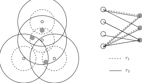
2.5 Two sensing ranges sensors and targets relations. . . 52
2.6 Sensors activation/deactivation. . . 53
2.7 Sensors node status. . . 54
2.8 Directional sensors. . . 56
3.1 a schduling formulation of WSNs lifetime optimization . . . 61
3.2 The method owerview . . . 63
3.3 Covers scheduling. . . 73 x
3.4 Genetic algorithm chromosome creation. . . 79
3.5 Genetic algorithm crossover strategies. . . 80
3.6 The Genetic algorithm Combinations . . . 81
3.7 The order crossover . . . 83
3.8 Rotated Crossover . . . 84
3.9 Genetic algorithm main stages. . . 87
3.10 GA Configurations . . . 88
3.11 DSC encoding in GA. . . 88
4.1 The number of cover for small and greater population size . . . 95
4.2 GA11 vs GA12. . . 105
4.3 Deterministic vs Randomize GA11. . . 106
4.4 The WSNs lifetime using SX, PMX, RX and OX crossover with p=10.107 4.5 WSNs lifetime using SX, PMX, RX and OX crossover with p=100. 107 4.6 The lifetime using one and two points mutations. . . 108
4.7 The lifetime using deterministic and randomized mutations. . . 108
4.8 The energy consumption via all sensors. . . 109
4.9 The 21 covers utilization via different number of generations. . . 109
4.10 Energy consumption by all sensors using SX, PMX, RX and OX crossovers. . . 109
4.11 The 21 covers utilization via different number of generations using SX, PMX, RX and OX crossovers.. . . 110
4.12 The lifetime for WSN with not identical sensors. . . 110
4.13 The DSCs for different numbers of sensors. . . 111
4.14 The DSCs for different numbers of iterations. . . 112
4.15 Crossover one-point randomized with different number of iterations. 113 4.16 Crossover two-point randomized with different number of iterations..114
4.17 Crossover one-point deterministic with different number of iterations..114
4.18 Crossover two-point deterministic with different number of iterations..115
2.1 Problem notations . . . 40
2.2 The sensor deployment and the targets positions . . . 42
3.1 Initial population . . . 86
4.1 The relation between the population size and number of NDSCs . . 94
4.2 The relation between the population size and number of NDSCs (ng=20) . . . 95
4.3 The WSN expandability . . . 95
4.4 GAMSC and GANDSC in ms . . . 96
4.5 SILSOM and ILSOM . . . 100
4.6 ILSOM for 10 sensors . . . 100
4.7 ILSOM for 20 sensors . . . 102
4.8 ILP model computation time samples . . . 102
4.9 Different GA mutation strategies . . . 104
4.10 GA and ILP based mettods comparison . . . 116
4.11 MSCGA and NDSCGA . . . 118
4.12 DSCGA and NDSCGA . . . 119
A wireless sensor network (WSN) is a collection of a vast number of small, low-cost, low-power and multi-functional sensor nodes deployed over a region or embedded in a target to be monitored or tracked. Each sensor node consists of a processing capability, a memory unit, an RF transceiver, an electrical battery as power source, and accommodate various sensors and actuators [8]. These nodes self-organize in
a cooperative network [9] to communicate and transmit the sensor measurements
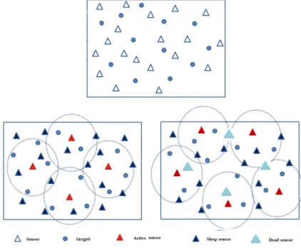
to the end user. The lifetime of each sensor node depends on the energy stored in the electrical battery. The sensor is considered to be dead once the battery is exhausted. Most of the applications of WSNs are intended to monitor a region or a set of targets. In some applications, targets may be located in a dangerous or remote area where installing sensors in specific positions can be a difficult or impossible task. In this case, sensors could not be accessed when installation is completed. For such difficult or impossible to deploy WSNs applications, sensors are randomly deployed in large numbers by flying an aircraft over the region to be monitored to ensure that the area or targets of interest could be covered. The network lifetime is defined as the time elapsed until any active sensor set fails to
satisfy the required coverage [10]. Possible primary states of a sensor in WSN
can be either active or in sleep, where active state consists of three possible states: transmitting signal, receiving signal and sleeping (or idle waiting for send/receive). To extend the lifetime of a sensors network, minimal subsets of sensors can actively cover the targets, while the other sensors can sleep. Then, the problem is to deter-mine how long to use a given subset and which subset to use next as a scheduling approach [11]. A significant number of researchers addressed the issue of efficient
energy management in wireless sensor networks considering the new constraints about sensing coverage introduced to satisfy the distributed nodes sensing
require-ments [12]. Powerful and modern optimal scheduling methods have emerged for
solving complex engineering optimization problems in the recent years regarding the various evolutionary computation methods addressed. These methods include mathematical programming techniques, genetic algorithms, simulated annealing, ant colony optimization, neural network-based optimization, fuzzy optimization, etc. The optimization problem can be solved by using decision data, the objective
function to be optimized and the constraints to be met [13]. In GAs, the term
chromosome is typically referred to a candidate solution for an optimization prob-lem, often encoded as a string of numbers, characters or bits. The genes are either single digit or short blocks of adjacent bits or characters that encode a particular element of the candidate solution [14].
Considering the WSNs application in which the sensors are not rechargeable, the battery lifespan is the available period of sensor node utilization. Therefore, the optimal lifetime for such WSNs is exactly the optimal utilization time of this lim-ited resources. For a set of sensors used to monitor a set of targets or region, subsets of sensors that satisfy the required monitoring should be found so as to be scheduled and implemented to prolong the network lifetime. The current work is an investigation for modeling and optimizing the life of such like set of sensors used for monitoring a set of targets or some fields. It aims to formulate the mathe-matical model of this problem through which the optimal energy utilization could be planned and the optimal lifetime could be obtained. This work tried to im-plement the mathematical programming and the evolutionary algorithm to build an efficient method for WSNs lifetime optimization, considering limited initial en-ergy for the involved sensor nodes. An integer linear programming (ILP) model is developed, and the GA is used in this work to solve the problem of randomly deployed wireless sensors network lifetime optimization formulated as scheduling problem.
The rest of this thesis is planned as follows:
WSNs, the scheduling, and the optimization theory. The WSN is described regarding the architecture, protocols, applications and research challenges. Then, the models, classes, environment, objectives, and complexity of the scheduling problems are presented. Finally, the optimization theory is in-troduced considering both exact and heuristic methods that are aimed to be implemented in this work. The most common exact methods of the linear programming (LP) and branch and bound (B&B) are briefly presented in addition to the most common heuristic and meta-heuristic methods such as greedy algorithm and genetic algorithms (GA).
• In chapter 3, we stated the problem of WSNs lifetime regarding the envi-ronmental constraints and the objective function to be maximized. Then, the most popular methods used to solve this problem in the literature are described. It is clear that the disjoint set cover maximization (DSC) problem is widely used to solve the WSNs lifetime optimization problem. Different exact and heuristic methods are used for WSNs lifetime optimization for-mulated as DSCs maximization problem. The WSNs lifetime problem is formulated in many different ways of mathematical modeling and different exact, and heuristic methods are used to solve it. One should notice that this problem in NP-hard.
• Chapter 4 details the method we developed using the non-disjoint set cov-ers (NDSCs) approach. For solving this problem, we split it into two sub-problems: 1) find the maximum number of NDSCs and 2) find the optimal scheduling that maximizes the WSNs lifetime. To find the optimal number of NDSCs we used a simple heuristic developed for this propose then worked out a GA based one. The second sub-problem started with the mathematical modeling of the problem then we developed an integer linear programming algorithm to find an optimal solution. Finally, we suggested and developed a GA for searching a near optimal solution in reasonable time. The GA based method coding, initialization, fitness, crossover, mutation, and selec-tion funcselec-tions are detailed. Several possible configuraselec-tions of the GA are possible based on four mutation strategies and for crossover operators.
State of the Art on WSNs
Scheduling and Lifetime
Optimization
1.1
Overview
This chapter aims to present an integrated vision of the problems incorporating the scheduling and the combinatorial optimization in the area of wireless sensor net-works. The wireless sensor networks (WSNs), the scheduling, the optimization and the recent research work in this scope should be explained. A general description of WSNs then, applications and the recent related research issues are considered. The scheduling area is briefly presented considering the models, the complexity, the algorithms and the operation. This chapter focuses on the combinatorial opti-mization methods including the exact methods, the heuristic and meta-heuristics, such as the integer linear programming and the genetic algorithms implemented in this work. To sum up, this chapter helps to understand the problem stated, with its related works in the next chapter.
1.2
Introduction to Wireless Sensor Networks
The sensing nodes are low-cost devices embodying a unit of digital signal proces-sors (DSP), with low-power radio frequency (RF) communication capability, and energy stored in a small battery [1] [2] (see figure1.1). The nodes have the ability to collect and communicate data to each other, or to a base station. Thus, each node can send data through the network for various utilizations such as monitor-ing, or decision support.Sensor ADC DSP RF Memory Battery
Figure 1.1: Wireless Sensor Node [1] [2].
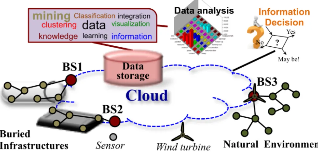
Sensor nodes communicate not only with each other but also with a base station (BS), using their wireless radios, allowing them to disseminate their data to re-mote systems of data processing, visualization, analysis, and storage. Figure 1.2
illustrates two sensor networks assigned to monitoring two distinct areas and con-nected through the intranet, using their base stations [15] [3]. Authors in [16] have described different interconnection architectures.
Cloud
Buried
Infrastructures Sensor Natural Environment
BS1
BS3
Data storage
data
mining Classification integration visualization learning
clustering
knowledge information
Data analysis Information Decision ? Yes No May be! Wind turbine
BS2
Figure 1.2: Sensors connected through internet via base stations.
In addition to the communication protocol layers (application, transport, network, data-link, and physical), the management (mobility, quality of service, security
and power management) challenges should be considered in the WSNs [17]. The
extended version of this standard was presented by Wang and Balasingham in [3]
as in figure 1.3.
The IEEE 802.15.4 standard specifies the physical layer and medium access control (MAC) layer characteristics of low power and low data rate radio communications used in WSNs such as the ZigBee standard. The features based on the IEEE 802.15.4 standard include data rates of 250 kbps, 40 kbps, and 20 kbps, two addressing modes (16-bit short and 64-bit IEEE for addressing), Carrier Sense Multiple Access with Collision Avoidance (CSMA-CA) is used for channel access. Fully handshake protocol for transfer reliability, power management for low energy consumption, 16 channels in the 2.4GHz ISM band, 10 channels in the 915MHz for the industrial, scientific and medical radio (ISM) band, and one channel in the 868MHz band [3].
Application Layer
Security Layer
Network Layer
Medium Access Control
Physical Layer The IEEE 802.15.4 standard
Figure 1.4: ZigBee Protocol Stack [3].
Based on the IEEE 802.15.4 standard, ZigBee is a low-cost, low-complexity and low power technology. The characteristics of this technology allow to developing full wireless mesh networks, involving up to 65,000 nodes in the wide range industry networks. It has network layer, security layers and application layers in addition
to the IEEE 802.15.4 standard (see figure 1.4). It has a global (2.4 GHz) and
various transmission options and security key generation mechanism based on the Advanced Encryption Standard (AES-128) security scheme [18] [19].
Different components and algorithms could be implemented in each of these layers, thus giving the opportunity to WSNs to be widely applied as an efficient link between the digital virtual world and the physical world. Efficient multi-channel media access control could apply to establish the nodes connectivity [4].
The ad-hoc networks [4], depicted in Figure 1.5, offered a flexible access medium, with greater energy efficiency, security, etc., while the capability Using custom routing control protocols. This kind of network is selected for a significant amount of research investigations and many applications [20] [21].
N1 N2 A B C D E F G H I
Figure 1.5: An ad-hoc networks [4].
The following subsections describe some of the WSNs applications, the research challenges, and the WSNs modeling. Also, the problem of lifetime optimization is introduced through the main factors affect the WSNs lifetime such as the energy, components degradation and failure.
1.2.1
WSNs applications
WSNs applications are increasingly penetrating into a broad range of the daily life and systems with a large variation in characteristics and requirements. Their operation relies on exchanges of data and information through different layers using protocol stacks with specific constraints and needs. So, to meet the increasing
needs of users and applications, [22] and solve the tough operating problems, close collaborations will be required between software developers, researchers, and hardware designers.
From service provider vision, a WSNs aims to provide the quality of service (QoS) required for the application layer, considering the physical and data link layer constraints. In a more abstracted vision, when the hardware constraints related to the application, the physical and data link layer, and the services are encapsulated, a service interface abstraction level is used for the interaction between the requests and the WSN, and the ad-hoc architecture may be presented as in figure 1.6 [5].
The application Service Interface Service Service Service Service The hardware
Figure 1.6: Application and a service interface [5].
The WSNs applications include environmental monitoring, industrial infrastruc-tures, civil infrastrucinfrastruc-tures, logistics, military, positioning and tracking, transporta-tion, medical applications, cyber-physical systems and the internet of things [5] [22].
• Environmental applications
The WSNs are intensively implemented in the environmental monitoring ap-plications such as weather, radiation and air pollution monitoring systems
[23]. The WSNs architecture and nodes should have the capability to
com-municate with each other, collect the environmental data from a region of interest and transmit the data via the gateway to the monitoring center in addition to the limited processing capability. The processing can mini-mize the invalid data transmission to reduce the overall energy consumption during data transmission. The WSNs can monitor several environmental parameters according to the application such as underground water level, pressure, temperature, wind direction and speed to provide various services for end users. The architecture of such systems is widely discussed, for in-stance in [24]. Autonomy, reliability, and flexibility are the most common requirements of such networks [25].
• Industrial infrastructures applications
Reliability, availability, maintainability, and mobility characteristics are cru-cial for the WSNs implemented in industrial infrastructures and automation applications. Tasks of events detection, periodic data collection, real-time data acquisition, equipment control, robots control and real-time inventory management have been assigned to WSNs. WSNs implementation has some advantages in industrial infrastructures compared to the wire communica-tions. The benefits include flexibility of installation and upgrading the net-work, lower costs of deployment and maintenance, decentralization of tasks automation, flexibility for moving and rotating devices, easier fault
diag-nosis. Possible interfaces to wide area networks from different networks
can help improving the efficiency of automation infrastructures. An addi-tional advantage is the high interconnection capability of integrated wireless sensors with built-in communication using micro-electromechanical systems (MEMS) [26].
WSNs is one main part of the modern military logistics, operations, and hu-man resources protection. The requirement and challenges of the WSNs de-sign depend on the operating scenarios for which they are intended. Most of the military applications are large-scale implementation in which the WSNs are non-manually deployed. Different sensor types are implemented in par-ticular WSNs for supporting defense strategies, environment surveillances, and logistics support [27].
• Medical and healthcare applications
High performance and reliability computational devices, smart sensors, and high sensitive measurements devices are required in WSNs architecture im-plemented in healthcare so as to allow in-home assistance or telemedicine and perform patient progress monitoring and emergency situations. Also, light or voice reminders could be used for the patient to remember the medical data and time [28].
• Transportation and mobile applications
The efficient traffic management systems are required to cope with the rapid increasing of traffics around the world, with accidents avoidance support. The WSNs used in intelligent transportation systems have introduced new ideas about the smart city applications with the capability to offer traffic safety and congestion control [29].
• Internet of things
Internet of things (IoT) is the capability of physical objects or things with embedded smart system to communicate and sense their internal and
ex-ternal environment. The WSNs are used to provide the communication
infrastructures for the IoT to introduce new applications, services, and the smart world. Figure 1.7 explains the IoT applications and future [6].
Figure 1.7: IoT future and applications [6].
Several applications and research challenges related to IoT are brought out and classified by Miorandi et al [7] as in figure 1.8 [7].
Security Trusted Platforms, Low-complexity, Encryption, Access control Privacy, Data confidentiality, Authentication, Identity management Energy harvesting, low energy computing
architectures, RFID Network protocols, Connection awareness,
Naming systems, etc Data representation,
Mining, Ob. virtualization, Profile managements, etc
Computing & Communication Distributed Systems Distributed Intelligence
Figure 1.8: IoT research challenges [7].
• Cyber physical systems
The Cyber-physical systems (CPS) are systems that integrate natural and human-made physical systems with computation, communication, and cy-bernetics as an interaction between physical and computational environ-ments. The sensing and sensor networks are the provider of the communica-tion and data colleccommunica-tion for the cyber-physical systems and its applicacommunica-tions [30] [31].
The characteristics and advantages of WSNs are still attractive for new appli-cations to be introduced. This large area of appliappli-cations has brought out more research challenges to be investigated in WSNs. The next paragraph introduces some of them.
1.2.2
Wireless Sensor Networks research challenges
The evolution of WSNs, which merged many fields with a broad scope of appli-cations and brought out many attractive issues, are addressed by intensive in-vestigations. The problems include localization, connectivity, coverage, obstacle adaptability, node density, communication and sensing range, energy, lifetime, sen-sor relocation, movement of sensen-sors, fault tolerance, reliability, ...[32] [17]. The next paragraphs present some of the WSNs research challenges.
• Deployment
For localization and deployment, the targeted object or field position should be known. Random deployment could be used by default to access envi-ronments. The sensor node could be efficiently used or not completely used according to its position [33]. Network cost, coverage, connectivity and
life-time constraints could be considered to optimize the WSNs deployment [34]
in addition to the targets mobility and tracking [35]. • Connectivity
Many protocols are developed recently as connectivity and routing strate-gies considering the dynamic topology of the WSNs to ensure the collected data propagation to the end destinations. For more details about routing protocols of mobile ad-hoc Networks, the reader can refer to [20] for example. • Coverage control
Many protocols were developed to providing a continuous and effective cov-erage for the area of interest or the region to be monitored as one of the
important research challenges faced in the WSNs [36]. A centralized con-trol and distributed concon-trol are the main visible strategies used in coverage control developed for the ad-hoc sensor network [22].
• Self-adaptivity
The self-adaptivity and the adaptability to obstacle typically come together when describing the WSNs behavior or responding to the environmental changes or barrier. The capability of the WSNs to reorganize itself with the new situation or adaptability ought to be considered in the WSNs deploy-ment and installation [37] that could support the fault-tolerance for WSNs based systems [38].
• Nodes density
The node density is used to describe the number of nodes allocated in the targeted field. It has a direct effect on all or most of the WSNs research challenges such as the connectivity, energy consumption, adaptability, re-siliency and lifetime. Considering that the node has the capability to act as sender and router, the power consumption in each node is affected by its position, the nodes near the base station spend more energy for data routing. Therefore, the node density should be greater in the neighborhood of a base station, or the sensing nodes will not be connected soon and so the node lifetime will be shorter [39].
• Communication range
For each node, the communication range is defined as the circle area “or section” inside which the neighbor nodes can receive its signal with a radius equal to r [40].
• The energy
The power management [41] is always considered in WSNs design regarding
the available energy amount used for sensor node operations. Typically, the sources of energy are batteries which must be replaced or recharged after the drain. For some nodes, both options are not applicable. Therefore, the sensor nodes will just be discarded once their energy reserve is depleted [15].
The efficient coverage control methods could optimize the energy utilization, the WSNs lifetime [42] and the number of nodes required for coverage [43].
The energy reserve, coverage control, node density, deployment are main factors to prolong the WSNs lifetime, availability and reliability. How can these factors affect the lifetime is described in details in the next chapter as the main problem of this work.
1.2.3
Wireless Sensor Networks description and modeling
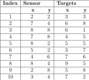
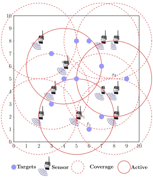
For every WSN, a limited number of sensor nodes are deployed in two-dimensional or three-dimensional space, for the surveillance of specific targeted objects or fields. The sensor nodes send the collected data to static or mobile base stations. There-fore, the deployment of the sensor node requires to specify the values of (x, y) of each node in the 2-dimensional space or (x, y, z) for 3 dimensions. Then, the capability of each sensor node to monitor all or part of targeted objects or fields mainly depend on this deployment and the coverage range r. Every sensor node i can monitor every target j, if the distance dij is less than or equal r. Figure 1.9 displays 10 sensor nodes deployed in 10x10 area with r = 1.5.
0 1 2 3 4 5 6 7 8 9 10 0 1 2 3 4 5 6 7 8 9 10 BS r Figure 1.9: WSNs deployment.
The connectivity and data transmission between sensing nodes also depend on deployment values (x, y) of the sender and receiver in addition to the positioning
of the base station (BS). The distance between sender and receiver dsr must be
less than or equal to r to ensure a possible connectivity to the BS.
1.2.4
WSNs lifetime optimization through energy
consump-tion
The WSNs lifetime, as one of the most significant design challenges [44], is exactly the time elapses until all available sensors couldn’t satisfy the required coverage constraint. The lifetime may be affected by different factors such as sensor degra-dation or failure and the available amount of energy. When the reserve of energy is not renewable, and the sensors is operating in some critical area or location [45], the reserve of energy become the most important factor. Therefore, the lifetime
of the WSNs could be optimized through optimization of energy consumption. In ad-hoc WSNs, the energy consumption depends on the data sensing rate, receiving and transmission rate[46] [47], which depend on the nearness of the node to the base station. Although there are many recent works regarding this problem, it has not been fittingly solved [48].
1.2.5
WSNs reliability, failure and self-adaptivity
Reliability is one of the most significant requirements for a wireless sensor networks applications in the areas of industry, healthcare, and environments. Reliability level of the network can be evaluated using reliability modeling and analysis as key steps for designing and optimization of sensor network systems. Whatever the strategy used for sending the sensed data to the end user, data cannot be delivered if the path fails, which may happen either in the communication link or the WSN node. A link failure can happen due to different factors such as noise, interference, distance, or environmental conditions. While, the WSN node can fail due to firmware factors (embedded operating system) or hardware factors (radio, sensors and energy devices) failures [49]. In [49] the reliability of a node is defined as sequential sorted blocks of all factors such as application, firmware, middleware, hardware, radio communication or battery level. As the reliability of a WSN node is a function of the reliability of its components arranged in series, if one of them fails, the whole node fails. Regarding the reliability, the WSNs design, and deployment [50] should consider sensor node constraints like battery power, transmission range, sensing range and processor capability. The energy, sensing, processing and communication issues should meet the reliability requirements, and the communication ought to consider the connectivity requirements so that the end user can access the network and receive the expected data sensed and processed by the sensing nodes. Achieving the overall network reliability of the communication process is to construct a network with the minimum number of reliable links and each link must be feasible [51]. The self-adaptivity has different definition[52]: it is the capability of the system to adapt its behavior according
to the environment or the ability of a system to achieve its goals in a changing environment, by selectively executing and switching between operating models. Therefore, a self-adaptive system evaluates its behavior and changes its operation when the evaluation indicates that its performance is not sufficient. Finding a better possible configuration or performance according to the most common stages is depicted in figure1.10. The tasks for self-adaptivity includes: monitoring of the targeted system or the environment to collect the conditions data required for adapt, analysis of the collected data to make adaptive decisions in the next-step, determine and plan the steps to achieve adaptivity, and execute the steps.
Monitoring
Executing
Planning
Analysing
Figure 1.10: The self-adaptivity common stages
At all time, the system components are monitored, the collected data analyzed and estimated to the required, and then the next operation strategy is planned “if available” and executed.
The WSNs lifetime should be optimized considering the limited energy reserve, the component degradation and the probability of failure constraints. An effi-cient resources utilization, tasks assigning and scheduling method could prolong the WSNs lifetime. The next subsection describes the scheduling environment, constraints, objectives and its applicability in WSNs.
1.3
Scheduling problem
Planning and scheduling as defined in [53] are decision-making processes that are used on a regular basis in manufacturing and services. Mathematical techniques
are utilized in all planning and scheduling functions. Solving a scheduling problem can consist to organizing a set of activities (jobs or tasks) to be executed, by using the available resources capacities. This execution has to consider and follow different technical rules (constraints) to achieve the maximum efficiency of the resources (according to a set of criteria or objectives) [54]. The number of jobs and the number of machines are assumed to be finite and denoted by n and m respectively. Then the pair (i, j) refers to the processing step or execution of job j on machine i. The following pieces of data are associated with job j [55]. The task index, processing time, release time and priority index are relevant variables in scheduling problem.
1.3.1
Modeling the scheduling problems in WSNs
The problem of scheduling in WSNs could be considered as follows:
Given a set of sensors and a set of targets, find the sensors assignment to targets
coverage that maximizes the total coverage time or more objectives. Figure 1.11
gives a suggestion of 5 sensors assigned to cover 4 targets.
T1 T2 T3 T4 s2 s3 s4 s5 s1 1 2 3 4 5 6 7 8 coverage time
Figure 1.11: Sensor to targets coverage scheduling
In figure 1.11, T3 is not covered through all coverage time while T1 and T2 are not covered for a part of the coverage time. In most cases, the scheduling part required after covers determining is left without solution [56] [57].
To ensure that all targets are covered all time, the possible number of covers should be found ”not necessary to be disjoint.” Then, one should search for covers to targets assignment to optimize the coverage time. Figure1.12gives a suggestion for 4 covers composed of 7 sensors assigned to cover 4 targets.
T1 T2 T3 T4 s7 s5 s6 s2 s1 s3 s4 s2 s4 1 2 3 4 5 6 7 8 coverage time
cover1 cover2 cover3 cover4
Figure 1.12: Covers to targets coverage scheduling
In figure 1.12, cover 1 includes S1 and S3, cover 2 includes S1, S2 and S4, cover 3 includes S4 and S5 and cover 4 includes S6 and S7. Therefore, this problem could be split into two sub-problems:
1. Given a set of sensors and set of targets, find the optimal covers.
2. Given a set of covers and a set of targets, find the coverage assignment that optimizes the coverage time.
In addition to the coverage, the parallel processing running on the collection of interconnected sensor nodes to execute a set of processes could be modeled as parallel machines, (see [58] for more details).
1.3.2
Scheduling environments, constraints, and objectives
The scheduling problem description is always composed of three parameters α, β and γ. The α field describes the machine and resources environment and contains
generally one entry. Tthe β field provides the necessary details about the process-ing constraints, and it can contain a sprocess-ingle entry, multiple entries or nothprocess-ing. The γ field describes the objective to be minimized and contains, in general, a single entry [55]. The possible situations of the machine environments specified in the α field are: 1) single machine (1) as the simplest of machine environment, algorithms such as weighted short processing time first (WSPT), weighted short discounted processing time (WSDPT) and earlier due date first (EDD) can be used to achieve the objectives, 2) parallel machines models in which a set of machines in parallel, widely applied in information systems, can be: identical machines in parallel (P m), machines in parallel with different speeds (Qm), or unrelated machines in parallel (Rm), 3) flow shop (F m) is a set of machines in series, each job has to be processed on each one of the machines. It could be generalized as flexible flow shop (F F c) when identical machines in parallel used in a subset of the series stages. 4) the job shop (J m) in which each job has its required route to follow in the environment, it could be generalized as a flexible job shop (F J c) when identical machines in parallel are used in a subset of the series stages. 5) the open shop (Om) determines a route for each job, different jobs could have different routes is allowed, some of the processing times on each one of the machines may be zero. The restrictions and constraints that could be found in β field includes: release dates, sequence dependent, preemption (prmp), precedence constraints (prec), representation as a directed acyclic graph (DAG), machine eligibility restrictions (M j), permutation (prmu), blocking (block), no ? wait (nwt) and recirculation (recirc).
Regarding the input variables of every scheduling problem (the environments (re-sources) variables and constraints), the scheduling problems aims to perform the following possible objective functions always to be minimized in the γ field [55]: 1) the makespan (Cmax) that defined as max(C1, ..., Cn), is equivalent to the time required for the last task to leave the system. Many approximation algorithms
developed for finding the minimum makespan of single machine [59] or parallel
environments. A minimum makespan usually refers to a good utilization of the resources, 2) the maximum Lateness (Lmax) that defined as max(L1, ..., Ln). It measures the worst violation of the due dates. This objective has been studied for
different applications and constraints through many algorithms as in [60], 3) total weighted completion time (P wjCj) which is the sum of the weighted completion times of the n jobs gives an indication of the total costs to be incurred by the schedule. The total weighted completion time or the weighted flow time is aimed to be minimized in many information system applications such as data centers [61], 4) the discounted total weighted completion time (P wj(1 − e−rCj)) is a more general cost function compared to the previous one, where costs are discounted at a rate of r, 0 < r < 1, per unit time. That is, if job j is not completed by time t, an additional cost wjre−rtdtis incurred over the period [t, t + dt]. If job j is completed at time t the total cost incurred over the period [0, t] is wj(1 − e−rt). The value of r is usually close to 0, say 0.1 or 10%. 5) total weighted tardiness (P wjTj) is also a more general cost function than the total weighted completion time, 6) weighted number of tardy jobs (P wjUj) is not only a measure of academic interest; it is often an objective in practice as it is a measure that can be recorded very easily. All the objective functions above are so-called regular performance measures.
1.3.3
Complexity of the scheduling and optimization
prob-lems
Solving a scheduling and optimization problem amount to finding the optimal or near-optimal solutions for the objective function considering some goals and restrictions. The complexity of the optimization problem could be evaluated based on the computational resources required to solve it considering both time and space complexity. The optimization problems are classified in different groups or complexity classes according to the computational efforts required to find the optimal solution. The problems in one complexity class could have limits linked to the computational complexity, which depends on the size n of the problem or its input size. the complexity classes includes the polynomial P , non-deterministic
polynomial N P , NP-complete and NP-hard [62] The complexity P class is a set
of optimization problems that can be solved in polynomial time complexity in the worst-case. The time required for solving effectively this problem in P is bounded
for any instance of the problem with n inputs (n > 0) by a polynomial function
of the type O(nk). The complexity N P class includes problems with practical
importance. It describes the set of optimization problems that can be solved in polynomial time in worst-case using a non-deterministic algorithm. The N P − complete belongs to N P , and there exist polynomial algorithms to transform every problem in N P into it. The N P − hard is not in N P but there is a N P − complete problem that can be transformed into it with a polynomial time. It is assumed that P is a subset of N P (P < N P ) whether some problems are in N P , but not in P . The Complexity classes relations are depicted in figure 1.13 [63] [64].
P NP-complete
NP-hard NP
Figure 1.13: Complexity classes.
1.3.4
Scheduling classes
In scheduling terminology, a sequence usually corresponds to the n task permuta-tion or the order of jobs processing on a given machine while the schedule usually refers to an allocation of tasks within a more complicated setting of machines that allows the possibly for preemptions of tasks by other tasks that may be released at a later time. Different scheduling classes with different operating conditions could be abstracted as in figure 1.14.
Semi − Active ActiveSchedule
N on − Delay
Figure 1.14: Scheduling classes.
A feasible schedule is called non-delay if no machine is kept idle while an operation is waiting for processing. Requiring a schedule to be non-delay is equivalent to preventing unforced idleness. A feasible non-preemptive schedule is called active if there is no possibility to construct another schedule, by changing the order of processing by the resources, with at least one operation finishing earlier and no operation finishing later. A feasible non-preemptive schedule is called semi-active if no operation can be completed earlier without changing the order of processing on any one of the resources.
1.4
Optimization approaches
Optimization problems are common in many fields and different domains in the human activities where we have to find an optimal or near-optimal solutions for specific problems with the capability to meet some limitations. The most common optimization problems characteristics include the following:
1) It has many alternatives of decision and possibilities of solution.
2) Additional constraints can limit and decrease this number of available alterna-tives.
4) It has an evaluation function that based on these alternatives described as func-tion of the decision variables [63].
Given a set of decision variables V = {v1, v2, ..., vv}, optimization considered to obtain the best solution for an objective function of this decision variables f (V ) according to some restrictions on the decision variables. The best solution is ob-tained either by minimizing or by maximizing the objective function, and the optimization consists of finding the condition of the decision variables that gives
the maximum or minimum value of the objective function. Figure 1.15 explains
that if a point vi ∈ V is approved with in the minimum value of the function
f (v), the same point is also confirmed in the maximum value of the opposite of the function, −f (x) [65] .
Figure 1.15: Maximization and minimization of f(v).
The optimization problem, in general, has the following mathematical formulation:
• The objective function
M aximize/M inimizef (v1, v2, ..., vn)
• The constraints
ϕj(v1, v2, ..., vn) ≤ 0(i = 1, ..., m)
This formulation is normally referred to as the general nonlinear programming problem. The feasible point of a solution is any point value of the vector V that satisfies all these equations [66].
1.4.1
Combinatorial optimization
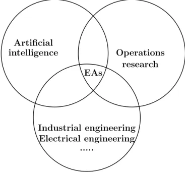
Combinatorial optimization methods are useful in a particular type of mathemat-ical optimization problem in which the set of feasible solutions of the problem is finite. Such a problem is defined, in its most general form, on a finite set of feasi-ble solutions with a reasonafeasi-ble characterization [67]. The computational problems normally require significant efforts to search a huge number of candidates for the optimal solution in which the evolutionary algorithms could be used. The evolu-tionary algorithms are natural principles based computational methods developed as a simulation of natural behavior to be implemented in computer science for human systems developing. This kind of algorithms is involved in many fields of research, development, and applications as in figure 1.16 [64].
Industrial engineering Electrical engineering ... Operations research EAs Artificial intelligence
The key features of the evolutionary algorithms include: 1) has group of solutions or individuals to be enhanced called Population (Population-based); 2) the solu-tions or individuals in a population have its value or representation (code), and the evaluation of this values is called its fitness value (Fitness-oriented); and 3) Variation-driven.
1.4.2
Optimization methods
This subsection aims to describe the methods, techniques or strategies used to solve the optimization problems in many fields of application. According to the quality of solution guarantee, these could be classified in exact and approximation or heuristics as in the next paragraphs.
1.4.2.1 Exact methods
This sub-section describes the exact methods that aimed to guarantee the optimal solution, even if it takes greater computational efforts regarding the resources and time. The exact methods include the Branch and Bound, the Branch and cut, the Simplex, etc. Several examples are described below in addition to the linear programming used in this work.
Linear Programming The common form of the linear programming is as
follows: M aximize f (x1, ..., xn) = c1x1+ c2x2... + cnxn (1.1) Subject to : n X i=1 aijxi ≤ bj∀j = 1, ..., m (1.2)
0 ≤ xi∀i = 1, ..., n (1.3) where m and n are given natural numbers, ci, bj and aij are constants and xi are decision variables. Expression (1.1) is the objective function to be maximized or minimized and expressions (1.2) and (1.3) are constraints. With one more charac-teristic that both the objective function and the constraints are linear equations or inequalities [68] [69]. For a linear programming problem with two variables as the simplest case, the optimal solution can be obtained by using a graphical method as in figure 1.17
a b
c
d Optimal
Figure 1.17: Graphical method for simple LP - unique solution.
In some cases, the optimum solution may not be unique for example in the case of parallel function as in figure 1.18.
a b c
d
Figure 1.18: Graphical method for simple LP - parallel function.
Branch and Bound The branch and bound method is one of the main
strate-gies used for solving discrete and combinational optimization problems. Regarding a combinatorial optimization problem a finite set of feasible solutions, the branch-and-bound deals with these feasible solutions in a systematic manner to find the optimal solution of the problem. It tries to solve the combinatorial problem by di-viding it into smaller problems and computing an upper and lower bounds for each of the smaller problems that may be employed to exclude parts of the solution set out of consideration [67]. The branch and bound method has three main steps: 1) selection, 2) branching and 3) bound, with an appropriate rule or function should be defined for each step. See [70] for applied branch and bound example.
1.4.2.2 Heuristics and meta-heuristics
For hard problems, the exact algorithm that can guarantee the global optimal solution within an acceptable time might not be possible. Thus many heuristic algorithms have been developed for finding faster near-optimal solutions. Heuristic algorithms can quickly generate a solution with acceptable quality. But there is no guarantee for an optimal solution can be obtained and the time to derive a solution is also long in some worst cases [64]. Recent years have brought out a significant growth in the development of heuristic procedures to solve optimization
problems. There are many motivations and reasons for using heuristic methods. 1) No method to resolve the problem to optimality is known; even if there exists an exact method to solve the problem, it cannot be implementable on the available computing hardware. 2) The flexibility of the heuristic methods compared to the exact methods. 3) The heuristic method could be used as part of a global procedure that aims to find the optimum solution to the problem. The good heuristic algorithms should have the following characteristics: 1) It can obtain the solution within reasonable computational effort; 2) The quality of solution should be high and should have a high probability to find the near optimal solution; 3) The probability of obtaining a far from optimal or a bad solution should be very low. The heuristics and meta-heuristics include the Genetic Algorithms, the Greedy Algorithms, the Simulated Annealing, etc. [67]. It is important to highlight some of them in the next subsection, especially the genetic algorithm that we developed and implemented in this work.
Genetic Algorithm It is common in computer science to search for a
fea-sible and acceptable solution of a decision support problem among a collection of candidate solutions. The genetic algorithm (GA) is an approach to solution
search introduced by Holland in the 1960s [14]. Compared to the evolutionary
programming strategies, Holland’s goal was not only to design algorithms to solve complex problems but also to study and develop methods inspired by the natural adaptation processes applied to computing. Thus, the GAs have become the most modern evolutionary computation research technique. All the genetic information in humans is stored in 23 pairs of chromosomes. Each of these chromosomes is composed of several parts called genes as in figure1.19. The genes code the prop-erties and the characteristics of an individual and determine the characteristics of the next generations, an interesting aspect of evolution [71].
Figure 1.19: Genes and chromosomes
The GA simply executes a number of iterations or generations of selection, mod-ification and update of a set of candidate solutions or population [72] as basic evolution cycle in figure 1.20
Selected parents
Present generation
New generation Selection
Modification and mutation
Replacement
Figure 1.20: A simple evolution cycle.
The principles of a simple genetic algorithm is an integration of terminologies (subfunction and steps) includes the encoding, populations, individuals, crossover,
mutation, selection, fitness, evaluation and iterations that are used in a specific
way to formulate a GA based method [73].
• The encoding process:
This is used to represent the solution into individual genes and chromosomes so as to be processed using GA operators and functions. It can be performed using bits (binary), octal encoding, numbers (integer, real), arrays or any other objects.
• Population:
A population is a set of individuals or candidate solutions. The initial pop-ulation generation consists of a given number of individuals equal to the population size. This initial population is usually created randomly in GAs to be used as starting point of the searching process.
• Fitness and selection:
The fitness function is used in genetic algorithms to calculate the value of the objective function or constraints for its individual. To calculate the fitness, the chromosome has to be decoded first, then use the objective function for the evaluation. The assessment gives an indicator, which corresponds to how the chromosome is close to the optimal solution. The purpose of the selection process is to find fitter individuals of the population to be used as parents for reproduction of the next generation.
• Crossover:
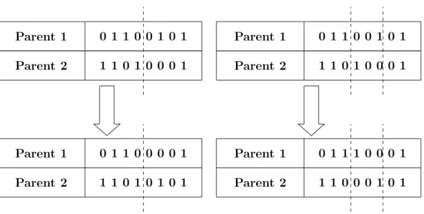
The crossover is the reproduction operator used for producing new children based on the selected parents. The parent’s offspring is typically composed of three steps: selects a pair of individual strings as parents, select the crossing at random along the chromosome length and finally, exchange the position values between the two strings according to the crossing points. Different types of crossover are developed such as single point crossover, two-point crossover, N-point crossover, uniform crossover, three parent crossover, or-dered crossover, partially matched crossover, etc. The single point crossover and two point crossover are depicted in figure 1.21
Parent 1 Parent 2 0 1 1 0 0 1 0 1 1 1 0 1 0 0 0 1 Parent 1 Parent 2 0 1 1 0 0 1 0 1 1 1 0 1 0 0 0 1 Parent 1 Parent 2 0 1 1 0 0 0 0 1 1 1 0 1 0 1 0 1 Parent 1 Parent 2 0 1 1 1 0 0 0 1 1 1 0 0 0 1 0 1
Figure 1.21: Single point crossover and two point crossover
For the partially matched crossover, for two with the same length, two crossover points are selected randomly and uniformly along the length. These crossover points give a possibility for a matching selection used to affect a crossover operator through position exchanges as in figure 1.22
Parent 1 Parent 2 0 1 1 0 0 1 0 1 1 1 0 1 0 0 0 1 Parent 1 Parent 2 0 1 1 1 0 0 0 1 1 1 0 0 0 1 0 1 Parent 1 Parent 2 0 1 0 1 0 0 0 O 1 1 1 0 0 1 1 1
• Mutation:
The mutation is used for preventing the algorithm from being trapped in a local optimal search. Different forms of mutation according to the various types of representation such as: reversing, interchanging, replacement, etc. [71]. The mutation can be done in general in two steps: genes selection and genes modification. The genes selection process is typically random, and many different modification functions are used according to problem nature and coding.
Many versions of GAs were developed such as parallel distributed GA, fine-grained parallel GAs (cellular GAs), multiple-deme parallel GAs, hybrid GA, adaptive
AG, fast messy GA and independent sampling GA [71]. The principles of a simple
genetic algorithm is depicted in figure 1.23.
Many heuristics were introduced and implemented in the literature including meth-ods such as, Greedy Algorithm, Ant Colony, and simulated annealing for example.
Simulated Annealing: This method was imported from the physical
anneal-ing process of heatanneal-ing up and coolanneal-ing down solid metals. The method was defined in combinatorial optimization and developed to finding a solution with a mini-mal cost from a large number of solutions. Thus, the simulated annealing (SA, for short) is a method designed for solving problems in the field of combinatorial optimization, by simulating the physical annealing process. The SA has many features such as the possibility of finding a high-quality solution, simple mathe-matical modeling and not need large computer memory. Furthermore, it is possible to start the SA with any given solution and try to enhance it which could be used to improve a solution obtained by other heuristic methods [66]. The exact, as well as the heuristic methods, have been suggested by researchers and implemented for solving the WSNs lifetime optimization problems, as will be presented in the next chapter.
Considering that the heuristics could not grantee the optimal solutions, there are many possibilities for the quality assessment of the heuristic base solutions. The
Start
Randomly generate the initial population
Fitness and selection
Crossover Mutation New generation Stop Yes No End
Figure 1.23: The simple genetic algorithm
later could be compared to an optimal solution, to an appropriate bound, or to other heuristics solutions [74]
![Figure 1.1: Wireless Sensor Node [1] [2].](https://thumb-eu.123doks.com/thumbv2/123doknet/14743487.755516/22.893.258.690.391.784/figure-wireless-sensor-node.webp)
![Figure 1.6: Application and a service interface [5].](https://thumb-eu.123doks.com/thumbv2/123doknet/14743487.755516/26.893.258.688.443.866/figure-application-and-a-service-interface.webp)