Linear and Nonlinear Rogue Waves in Optical Systems

HAL Id: tel-01508853

https://tel.archives-ouvertes.fr/tel-01508853

Submitted on 14 Apr 2017

HAL is a multi-disciplinary open access

archive for the deposit and dissemination of

sci-entific research documents, whether they are

pub-lished or not. The documents may come from

teaching and research institutions in France or

abroad, or from public or private research centers.

L’archive ouverte pluridisciplinaire HAL, est

destinée au dépôt et à la diffusion de documents

scientifiques de niveau recherche, publiés ou non,

émanant des établissements d’enseignement et de

recherche français ou étrangers, des laboratoires

publics ou privés.

Shanti Toenger

To cite this version:

Shanti Toenger. Linear and Nonlinear Rogue Waves in Optical Systems. Optics / Photonic. Université

de Franche-Comté, 2016. English. �NNT : 2016BESA2029�. �tel-01508853�

Thèse de Doctorat

é c o l e d o c t o r a l e s c i e n c e s p o u r l ’ i n g é n i e u r e t m i c r o t e c h n i q u e s

U N I V E R S I T É D E F R A N C H E - C O M T É

n

Linear and Nonlinear Rogue Waves

in Optical Systems

Vagues Scélérates Linéaire et Non-linéaire

dans les Systèmes Optiques

Thèse de Doctorat

é c o l e d o c t o r a l e s c i e n c e s p o u r l ’ i n g é n i e u r e t m i c r o t e c h n i q u e s

U N I V E R S I T É D E F R A N C H E - C O M T É

THÈSE présentée par

S

HANTI

T

OENGER

pour obtenir le

Grade de Docteur de

l’Université de Franche-Comté

Spécialité

: Optique et Photonique

Linear

_{and Nonlinear Rogue Waves}

in

_{Optical Systems}

Vagues Scélérates Linéaire et Non-linéaire

dans les Systèmes Optiques

Soutenue publiquement le 27 Juin 2016 devant le Jury composé de :

JÉRÔME

K

Rapporteur

Professeur à l’Université de Genève

M

Rapporteur

Professeur à l’Université de Lille 1

GOËRY

G

Examinateur Professeur à l’Université technologique de Tampere

MARC

H

Examinateur Professeur à l’Institut d’Optique Graduate School

M

Examinateur Professeur à l’Université de Franche-Comté

M. D

Examinateur Professeur à l’Université de Franche-Comté

It would not have been possible to write this doctoral thesis without the help and support of people around me, to only some of whom it is possible to mention here.

First and foremost, I would like to thank my supervisor, Prof. John M. Dudley, who had offered the opportunity to work in this fascinating, interdisciplinary area of research. During these three and a half years, I have learned a lot, not just from the academic point of view but also in many aspects of life. I am truly grateful for his invaluable guidance, encouragement, and example, from where I have learned the importance of focus, efficiency, and discipline in giving one best contribution. My sincere appreciation in particular for his support, patience, and understanding during this period of research.

I would like to thank all of the collaborators who contributed to the work included in this thesis, in particular Prof. Goëry Genty and Prof. Frédéric Dias, who have supported the completion of this work with their expertise. I also thank other collaborators, Minh, Cyril, Luc, Amaury, Mikko, Benjamin, Thomas, Yves, Miro, Thibaut, Jean-Marc, Laurant, Pierre-Ambroise, some of whom I have had the opportunity to work with and to learn from, both for the experimental work in the lab and the numerical simulations. My sincere gratitude also to my dissertation committee, Professors Hervé Maillotte, Jérôme Kasparian, Arnaud Mussot, and Marc Hanna, for their insightful comments, questions, and for letting my defense be an enjoyable moment.

I would also like to take this opportunity to record my sincere thanks to several people for their significant contributions to the completion of this thesis. I am especially grateful for the assistance given by Imad Faruque during the time this thesis was being written up. His support and guidance have been a great encouragement to the completion of this thesis. Special thanks to Rachel Yates for the generous time she has spent to proof-read this manuscript. Her prompt feedback has improved the quality of the manuscript and speeded up the writing process.

I am very grateful for all the amazing friends I have here during this period of time, who have made Besançon my home. The lab has been a wonderful place surrounded by warm and open-hearted people. Great time spent inside and outside of the lab, having lunch and sometimes dinner together, countless fun and enjoyable moments spent together not only with the fellow students in Optics but also with those from MN2S department is something I will always remember. I also thank those with whom I have shared the office most of the time, Irina, Bicky, Souleymane, Remi, Ismail, who have made the office a comfortable and stimulating place to work. Outside the lab, I am especially grateful for the community of Bonne Nouvelle church and Groupe Biblique Universitaire, who have always been very welcoming and caring. Your love and patience have also made the language difference not to be a barrier but a truly enjoyable moment of learning.

Finally I would like to thank my parents for their support and encouragement throughout my life. I am grateful to be raised in a family that values curiosity, passion, and freedom. Especially I dedicate this work to my mother who has always been a great example and a good friend.

List of Figures xi

List of Tables xix

1 Introduction 1

1.1 Outline of the thesis . . . 2

2 Rogue waves in the ocean and in optics 5 2.1 General introduction to rogue waves . . . 6

2.2 Rogue wave statistics . . . 8

2.2.1 Deviation of distribution from the standard model . . . 9

2.2.2 Classification of extreme events as rogue waves . . . 12

2.3 Oceanic rogue waves . . . 12

2.3.1 Linear mechanisms . . . 13

2.3.2 Nonlinear mechanisms . . . 15

2.4 Optical rogue waves . . . 19

2.4.1 Linear mechanisms . . . 20

2.4.2 Nonlinear mechanisms . . . 23

2.5 Optical - oceanic rogue waves comparison . . . 28

3 Rogue waves in a linear optical system 31 3.1 Experimental setup . . . 31 3.2 Two-dimensional focussing . . . 33 3.3 Three-dimensional focussing . . . 35 3.3.1 Numerical modeling . . . 35 3.3.2 Experimental results . . . 41 vii

3.3.3 Statistical properties and rogue waves . . . 42

3.4 Generation of an “Optical Sea” . . . 44

3.5 Conclusions . . . 47

4 Rogue waves in spontaneous modulation instability 49 4.1 Modulation instability and breather solutions . . . 50

4.1.1 First-order solutions . . . 50

4.1.2 Higher-order solutions . . . 53

4.2 Noise-driven modulation instability simulations . . . 55

4.3 Spontaneously emergent breathers . . . 57

4.4 Temporal-spectral correlation . . . 60

4.5 Statistical analysis . . . 61

4.5.1 Spatio-temporal dynamics . . . 61

4.5.2 Temporal dynamics at fixed distance . . . 63

4.6 Conclusions . . . 67

5 Real-time temporal measurement of spontaneous modulation instability 69 5.1 Space-time duality . . . 70

5.2 Generation of spontaneous modulation instability on a continuous wave . . . 74

5.3 Real-time temporal measurement using time-lens . . . 75

5.3.1 Time-lens based on four-wave mixing . . . 75

5.3.2 Experimental setup . . . 76

5.4 Experimental results and statistical analysis . . . 79

5.4.1 Spontaneously emergent breathers . . . 80

5.4.2 Statistical analysis . . . 81

5.5 Conclusions . . . 81

6 Stimulated modulation instability in optical fibres 83 6.1 Experimental setup . . . 84

6.2 Spontaneous, coherent seeded, and partially-coherent seeded MI . . . 85

6.2.1 Shot-to-shot MI spectral fluctuations . . . 86

6.2.2 Sideband noise suppression . . . 87

6.2.3 Effect on pump noise . . . 89

6.3.1 Wavelength dependence . . . 90 6.3.2 Bandwidth dependence . . . 92 6.4 Conclusions . . . 94 7 Conclusions and discussions 95 7.1 Conclusions . . . 95 7.2 Discussions . . . 97

Bibliography 99

A Some theoretical results 117 A.1 Transformation between different forms of NLSE . . . 117 A.2 Properties of elementary breather structures . . . 119

B Numerical Methods 123

B.1 The angular spectrum of plane waves . . . 123 B.2 Phase retrieval algorithm . . . 123 B.3 The split-step Fourier method . . . 125 C Explicit form of higher-order breathers 127 C.1 Collision of ABs . . . 127 C.2 Higher-order rational solutions . . . 129

2.1 (a) The Great Wave off Kanagawa depicting rogue waves emergence. (b) Example of rogue wave in the form of “wall of water” emerging in the ocean. (c) The surface elevation time history of the Draupner wave measured by a down-looking laser device. Source: from Ref. [1]. . . 6 2.2 Illustration of ocean surface wave characteristics (extracted from a small portion

of Draupner wave plotted in Fig. 2.1). The surface elevation ⌘ is the elevation of water surface above or below the reference level (average level); ⌘c is the height of

the crest (the point of maximum elevation); H is the wave height, defined either as the distance from the crest to the trough (down-crossing) H , or the distance from the trough to the crest (up-crossing) H+; T is the average wave period and h is the

water depth. . . 10 2.3 Probability density function of measurement data recorded from the Sea of Japan

[2] (black), fitted with the predicted distributions. (a) Surface elevation data and a Gaussian fit. (b) Wave height data and a Rayleigh fit. Both functions are plotted on linear and logarithmic scales (inset). Both distributions are normalised to the root-mean-square surface elevation ⌘rms. Source: from Ref. [3]. . . 10

2.4 Examples of heavy-tailed distributions commonly reported in the study of optical rogue waves, compared to an exponential distribution. . . 11 2.5 (a) Crossing sea, superposition of two wave systems travelling at different directions.

(b) Study of wave energy density in a random refracting field for an initial set of parallel rays corresponding to a single plane wave: (i) The random velocity field acting as random refracting medium (darker shades indicate higher velocity); (ii) The focussing of uniform plane wave passing through the random refracting medium from top to bottom (darker areas correspond to higher energy density). Source: from Ref. [4]. . . 14 2.6 Modulation instability: amplification of a weak modulation imposed on a harmonic

wave by nonlinearity, leading to the generation of spectral-sidebands through four-wave mixing process. . . 17 2.7 Modulation instability gain spectrum in hydrodynamics. . . 18

2.8 Linear rogue waves experiment. (a) Experimental set-up used to investigate rogue waves in the speckle pattern at the output of a multimode fibre. A spatial light modulator (SLM) is used to control the input beam profile. (b), (c) Measured speckle patterns (centre) and corresponding intensity distributions taken at a selected y-coordinate (right) when the SLM transmission mask (left) is uniform (b) and inhomogeneous (c). An optical rogue wave is observed in (c). Source: from Ref. [5]. . . 21 2.9 Modulation instability gain spectrum in optics. . . 27 2.10 The NLSE describes wave evolution in different physical systems. (a) Wave group

envelope u on deep water. (b) Light pulse envelope A in an optical fibre with anomalous group velocity dispersion. The figure illustrates solitons on finite background (top) and solitons on zero background (bottom). Note that for the ocean wave case, there is always deep water underneath u(z, t). For the water wave NLSE, k0 is the wave number and !0 is the carrier frequency; for the fibre NLSE, 2 < 0is the group velocity dispersion and is the nonlinear coefficient. Source:

from Ref. [6]. . . 29 3.1 Experimental setup. An SLM encodes random spatial phase on a coherent beam

from a He-Ne laser. Free space propagation transforms this random phase to random intensity spatial fluctuations. An imaging system is used to reduce the size of the beam so that it can be recorded on a CCD camera which can be translated longitudinally over an extended measurement volume. All measurement distances given in the text are relative to the origin z = 0 of the axes shown. Here f1= 500

mm, f2= 250mm, f3= 100mm, f4= 9mm. . . 32

3.2 Numerical simulations of one-dimensionally phase modulated beam with (a) weak phase modulation of 2⇡ and (b) strong phase modulation of 10⇡. For each case, (i) shows the applied phase distribution to the SLM; (ii) shows the unwrapped slice of the applied phase distribution along y-direction; (iii) shows the two-dimensional evolution of the refracted light observed in yz-plane; (iv-vi) shows the slice of the intensity distribution at different location along z, highlighting the contrast of the intensity distribution before, during, and after an extreme focussing. The intensity here is normalised to the intensity of incident beam. . . 34

3.3 Numerical simulations of two-dimensionally phase modulated beam with (a) weak phase modulation of 2⇡ and (b) strong phase modulation of 10⇡. For (a) and (b), (i) shows the applied phase distribution to the SLM; (ii) shows the unwrapped slice of the applied phase distribution at x = 0; (iii) plots the evolution of the maximum intensity of the spatial patterns along the propagation distance z. Black solid curve plots the evolution for the phase mask plotted in (i), while blue dotted curve plots the evolution of the averaged maximum intensity calculated from 10 different phase masks with the same 'max. Vertical red dashed lines correspond

to the locations from where each intensity patterns plotted in Fig. 3.4 and 3.5 are taken. (c) The maximum intensity Icaustic (green asterisks) and the distance to the

caustic regime zcaustic(purple open circles) as function of phase modulation strength

'max. The solid curves are the approximated functions, Icaustic = 1.85 'max (green

line) and zcaustic = 314 /'max mm (purple line). The intensity here is normalised

to the intensity of the incident beam. (d) Speckle contrast ⇢ as function of phase modulation strength 'max. The curves plotted in (c) and (d) are averaged from 10

different phase masks for each 'max. . . 37

3.4 Numerical simulations with phase modulation of 'max = 2⇡ taken at two different

regimes: (a) caustic regime and (b) speckle regime. The caustic network formed in this case has low contrast structures and the speckle pattern is partially developed. For each case, (i) shows the computed intensity distribution; (ii) shows a zoom over a more limited region (the highlighted region in (iii)) looking down on the pattern; (iii) shows a slice of the intensity distribution taken at x = 0 (indicated by the dotted line in (ii)); (iv) shows the calculated spatial spectrum corresponding to the intensity distribution in (iii). The intensity here is normalised to the intensity of incident beam. . . 39 3.5 Numerical simulations with phase modulation of 'max= 10⇡ taken at two different

regimes: (a) caustic regime and (b) speckle regime. The caustic network formed in this case is significantly sharper than the one in Fig. 3.4 and the speckle pattern is fully developed. For each case, (i) shows the computed intensity distribution; (ii) shows a zoom over a more limited region (the highlighted region in (iii)) looking down on the pattern; (iii) shows a slice of the intensity distribution taken at x = 0 (indicated by the dotted line in (ii)); (iv) shows the calculated spatial spectrum corresponding to the intensity distribution in (iii). The intensity here is normalised to the intensity of incident beam. . . 40 3.6 Experimental results contrasting (a) partially-developed speckle and (b) a caustic

network. For each case, (i) shows the recorded intensity distribution; (ii) shows a zoom over a more limited region (highlighted region in (iii)) looking down on the pattern; (iii) shows a slice of the intensity distribution at x = 0 (indicated by the dotted line in (ii)); (iv) shows the calculated spatial spectrum corresponding to the intensity distribution in (iii). The intensities shown here are normalised relative to the maximum intensity for the partially-developed speckle in (a). . . 42

3.7 Probability distributions of intensity calculated over all field points (taken within the beam profile area) of the simulation results shown in Fig. 3.4 and 3.5. The figure plots the statistical distributions of phase modulated beam with (a) 'max= 2⇡and

(b) 'max= 10⇡. For each, the statistics between the intensity patterns taken in the

caustic regime (black circles) and in the speckle regime (blue asterisks) are compared. 43 3.8 Probability distributions from intensity peak analysis of (a) partially-developed

speckle pattern and (b) caustic network. For each, the statistical distributions computed from the simulation results (black circles) are compared to the one of the experimental results (red asterisks). The black dashed lines correspond to the rogue wave intensity criterion IRW calculated from the numerical simulation

results, while the red dashed lines correspond to the criterion calculated from the experimental results. . . 44 3.9 Experimental results showing a spatial pattern with resemblance to a random sea

surface, which we refer to as an “optical sea”. (a) Shows the applied SLM phase. (b) Measured intensity pattern at 220 mm, presented in a similar way as above. The intensity here is also normalised relative to the maximum intensity for the partially-developed speckle in Fig. 3.6(a). (c) Shows (i) the retrieved amplitude pattern; (ii) a slice taken at the position where the highest peak A with amplitude ⇡ 2.23 is observed, dashed line in (i); Computed statistics of (iii) elevation and (iv) wave height. The solid lines in (iii) and (iv) plot Gaussian and Rayleigh distribution fits respectively. The label HRW indicates the rogue wave height threshold. . . 45

4.1 SFB solutions derived from Eq. 4.2 for different values of the parameter a as indicated: (a) Akhmediev breather (AB). (b) Peregrine soliton (PS). (c) Kuznetsov-Ma (KM) soliton. (d) and (e) second- and third-order solutions for the case of maximum intensity (the rational solutions). . . 50 4.2 (a) Modulation instabiility gain as a function of modulation frequency ! and

parameter a. Dashed lines indicate the modulation frequency at maximum MI gain (a = 0.25) and the cut-off frequency. (b) The evolution of temporal period ⌧, temporal pulse width ⌧, and maximum intensity of AB structures as a function of parameter a. The red circles indicate the values of these quantities at the maximum of MI gain (a = 0.25). . . 51 4.3 Schematic representation of the interrelation between various first-order solutions of

the NLSE (adapted from Ref. [7]). . . 53 4.4 Different types of second-order breather structures that are constructed from

different combinations of two AB collision with parameters shown in Table4.1. The maximum intensity in all cases is close to 15. . . 54

4.5 (a) Density map showing a small portion of the long term temporal evolution of a spatio-temporal MI field triggered by one photon per mode noise superimposed on a plane wave background. Local regions highlighted by white dashed lines correspond to the intensity profiles shown in Fig. 4.6. (b) Density map of the corresponding frequency evolution. Bottom subfigures plot evolution over ⇠ = 0 to ⇠ = 34; top subfigures plot evolution over a range around ⇠ s 283000. (c) The spectral cross section at different distance ⇠ along the propagation, contrasting the MI spectra at the initial stage ⇠ = 5.5, at a ttypical MI spectral broadening ⇠ = 26.3, and at the emergent of extreme collision of three ABs ⇠ = 283211.5. . . 56 4.6 The gray shaded plots show the intensity profiles extracted from the regions of the

chaotic MI field indicated in Fig. 4.5 for an AB, PS, KM, second-order superposition

2, and third-order superposition 3 respectively, compared with the corresponding

analytical NLSE solutions (red solid line). . . 57 4.7 Scatter plot of temporal width (FWHM) against peak intensity for the 2853669

intensity peaks in the chaotic MI field from simulations (gray circles) compared with theoretical predictions for the properties of SFBs (red solid line). A comparison is also made with a power function of ⌧fit = 1.678/(| |2max)0.532 (blue dotted-dashed

line). The peak intensities of the spontaneously emergent localised structures are obtained using specific peak detection over a full two-dimensional spatio-temporal computational window, and their corresponding temporal widths are calculated in the same way as the calculation done for the analytical SFB structures explained in Appendix A.2. In the bottom panel, we plot several examples of spatio-temporal structures of the spontaneously emerging breathers to highlight the nature of the breathers typically found around the region. These breathers correspond to the temporal intensity profiles plotted in Fig. 4.6(a,b,d,e). . . 59 4.8 As a function of the propagation distance ⇠, (a) and (b) plot the evolution of the

width of the autocorrelation coherence peak and the 80 dB spectral width for the evolving MI field in Fig. 4.5. These results illustrate how spectral expansion is associated with the appearance of shorter temporal structures in the random AB pulse train. (c) and (d) show the autocorrelation and spectrum for the highest intensity peak associated with the collision between three breathers. The detail in (c) shows how the FWHM of the central autocorrelation coherence peak is determined. 60 4.9 (a) Peak intensity statistics of the localised structures. (b) Distribution over the

complete field intensity of the two-dimensional spatio-temporal computational window. The dashed lines indicate the Peregrine soliton threshold IPS | PS|2max and the rogue intensity threshold IRW. Both distributions are plotted on

semi-logarithmic scale. . . 62 4.10 (a) Peak amplitude statistics obtained using the same peak detection method as

used in Fig. 4.9. (a) Distribution over the complete field amplitude of the two-dimensional spatio-temporal computational window. The dashed lines indicate the Peregrine soliton threshold APS (| PS |max)and the rogue amplitude threshold ARW. Both distributions are plotted on semi-logarithmic scale. . . 63

4.11 Statistical analysis of temporal dynamics of intensity envelope taken at distance ⇠ = 250 of simulated MI chaotic field. (a) Plots a small section of the intensity envelope fluctuation, with the distributions plotted in (b) taken over the whole intensity fluctuation and (c) taken only from the temporal intensity peaks (37385 temporal peaks are detected by applying relative minimum threshold of 0.4). The black dashed line indicates the rogue intensity threshold IRW. For a comparison,

dotted blue dashed curve plots the distributions of the spatio-temporal field intensity and peak intensity shown in Fig. 4.9. . . 65 4.12 Statistical analysis of temporal dynamics of modulated carrier wave taken at

distance ⇠ = 250 of simulated MI chaotic field. (a) Plots a small section of the modulated carrier wave (extracted from the intensity envelope that is highlighted in gray shaded area in Fig. 4.11(a)). (b) Plots the distributions of the wave fluctuation (corresponding to surface elevation of an ocean wave), and (c) plots the distribution of the wave height. The red solid lines plot the Gaussian and Rayleigh fit of the distributions. The black dashed line indicates the rogue wave height threshold HRW. . . 66

5.1 The space-time duality of diffraction and dispersion in the far-field regime. (a) Describes diffraction of a monochromatic beam resulting in the broadening of the beam profile. (b) Describes dispersion of a light pulse resulting in frequency chirp that broadens the pulse. In both cases, the far-field propagation leads to the Fourier transform of the input waveform (frequency-to-time conversion process). Adapted from Ref. [8]. . . 71 5.2 (a) The analogy between spatial and temporal imaging. A spatial magnification

is realised by cascading input diffraction, lens, and output diffraction. Whilst a temporal magnification is realised by cascading input dispersion, time-lens, and output dispersion. (b) Spatial and temporal magnification in the limit of large magnification. The system can be seen to be constructed by a 2f Fourier processor time-to-frequency conversion realised by a temporal 2f Fourier processor, followed by a far-field frequency-to-time conversion. Here uin, uF P, and uout denote the

input, Fourier plane, and output electric field respectively, and ˜Uin, ˜UF P, and ˜Uout

denote the corresponding Fourier transform. Source: from Ref. [8]. . . 73 5.3 Time-lens system based on FWM. A signal wave is mixed with a linearly chirped

(stretched) pump pulse through FWM process, generating an idler wave which is a replica of the input wave with an imparted quadratic phase. Here us, up, and ui

denote the electric field of the signal, pump, and idler respectively. Source: from Ref. [8]. . . 76

5.4 Experimental setup of the real-time temporal measurement of spontaneous MI on CW signal using ultrafast temporal magnifier (Picoluz UTM-1500). (a) The generation of the spontaneous MI on CW field. (b) The preparation of the ultra-short pump pulses. (c) The FWM based time-lens magnifier system. The signal and the idler were passed through dispersive propagation steps (Din and

Dout), before and after the time-lens system, respectively. The pump pulses were

passed through dispersive propagation Dp before being combined with the signal

in the silicon waveguide (Si-WG). This cascade process of the input dispersion, FWM based time-lens, and the output dispersion allows the signal waveform to be temporally magnified. (d) Illustration of the real-time temporal magnification process. (i) The temporal intensity profile of the breather structures with typical width T ⇡ 3 ps. (ii) The linearly chirped pump pulses used to realise the time-lens system. (iii) The magnified breather structures (76.4⇥) ready to be measured by the ultrafast oscilloscope. The record length M T ⇡ 5 ns and refresh rate fr = 100 MHz of the magnified waveforms are determined by the

pump pulses. . . 77 5.5 Intensity profiles obtained from the time-lens measurements (top, red) and

simulations (black, bottom) at two different fibre length: (a) 11.7 km and (b) 17.3 km. Measured intensities P are normalised with respect to the mean output background intensity hP i, plotted against the rescaled (demagnified) time. Experimental results from several measurement windows (indicated by dashed vertical lines) are concatenated for comparison with simulation. . . 79 5.6 (a) and (b) show scatter plots of pulse duration against normalised power from the

intensity profiles obtained from the experiments (top, red points) and simulations (bottom, black points), taken at 11.7 km and 17.3 km propagation distance respectively. For each case, the theoretical curve calculated from the elementary and higher-order breather solutions is also plotted as comparison. The figures on the right panel plot the intensity profiles extracted from the experimental results (red lines) compared to the analytical fits (black lines) for (c) P/ hP i ⇡ 9 and (d) P/hP i ⇡ 13. . . 80 5.7 Histograms (probability density) of the peak intensities from the spontaneous MI

pulses taken at propagation distance of (a) 11.7 km and (b) 17.3 km. The inset plots the histogram on semi-logarithmic axes. For each case, the histogram obtained from the experiment (red) is compared to the one from simulation (black). The dashed blue lines indicate the rogue wave intensity threshold IRW. . . 81

6.1 Experimental setup of coherent and partially-coherent seeded MI. A tunable continuous wave (CW) laser is used for the coherent source, while a filtered amplified spontaneous emission (ASE) was used for the partially-coherent source. The real-time (shot-to-shot) MI spectra are measured by using dispersive time stretching technique. EDFA: Erbium-doped fibre amplifier, WS: waveshaper, PC: polarisation controller, HNLF: highly nonlinear fibre, DCF: dispersion compensating fibre, OSA: optical spectrum analyser, FROG: frequency-resolved optical gating. . . 84

6.2 Simulation results. Bottom panel plots MI spectra for (a) no seed, (b) CW seed at 1531 nm, (c) 1 nm bandwidth ASE seed at 1531 nm. The spectral broadening in (a) is the results of spontaneous MI (noise seeded), while (b) and (c) are results of stimulated MI. Individual realisations are shown in gray (superposes 500 spectral traces) with the average in black. Vertical red and blue dashed lines indicate the wavelength of the first and second MI sideband, from where the distributions shown in Fig. 6.3 are taken. Upper panels show second-order spectral coherence and coefficient of variance Cv. . . 86

6.3 Histograms data of spectral fluctuations from first sideband at wavelength 1580 nm (top) and second sideband at wavelength 1607 nm (bottom). For each wavelength three cases of MI spectra are shown, for (a) no seed, (b) CW seed, (c) 1 nm bandwidth ASE seed. The histograms are calculated from 5000 realisations of the simulation data. . . 88 6.4 Calculated second-order moment (skew ) and third-order moment (kurtosis ) of

the MI spectra for (a) no seed, (b) CW seed, (c) 1 nm bandwidth ASE seed. Vertical red and blue dashed lines indicate the wavelengths corresponding to the distributions shown in Fig. 6.3. . . 88 6.5 Seeding effect on spectral fluctuations of coherent pump. Upper panels show the

calculated normalised third-order moments (skewness ) and the spectra around the pump wavelength. Lower panels show the histogram data at wavelength 1553 nm and 1556 nm. The histograms and the skewness are calculated from 5000 realisations of the simulation data. Comparison is made for (a) no seed, (b) CW seed, (c) 1 nm bandwidth ASE seed. . . 90 6.6 (a) MI spectral profiles as ASE seed wavelength is varied. The MI gain curve is

shown beside the experimental density plot. (b) Experimental average spectra taken from 5000 single-shot spectra (solid) and numerical average spectra taken from 5000 numerical realisations (dashed) for unseeded (top) and for a 1531 nm seed (bottom). (c) Seed wavelength dependence of 30 dB MI bandwidth (top) and Cvat 1580 nm

(bottom). . . 91 6.7 (a) MI spectral profiles as CW seed wavelength is varied. The MI gain curve is shown

beside the experimental density plot. (b) Experimental average spectra (solid) and numerical results (dashed) for unseeded (top) and for a 1531 nm seed (bottom). (c) Seed wavelength dependence of 30 dB MI bandwidth (top) and Cv at 1580 nm

(bottom). . . 92 6.8 Experimental results showing the variation with ASE seed bandwidth centered at

wavelength = 1531 nm of (top) 30 dB MI bandwidth and (bottom) Cv at 1580

nm. . . 93 A.1 Temporal profiles of AB solutions for different a parameter: (a) 0.1, (b) 0.125, (c)

0.25. . . 120 B.1 Schematic of phase retrieval algorithm used to reconstruct the amplitude

2.1 Rogue waves in different optical systems . . . 20 4.1 Different combination of parameters corresponding to the plot of second-order

breathers shown in Fig. 4.4. . . 54

Introduction

We experience randomness in many aspects of our lives. In most cases, the random fluctuations vary over a limited range around some average value, and higher events occur with significantly lower probability, to the extent where their occurrence can be ignored. However, in some cases, events which are far from the average occur more frequently than expected. For example, studies show that typically around 20% of a population owns 80% of the wealth, or 20% of products (or customers) bring in 80% of the revenue, which is known as the Pareto principle [9–11]. In this case, the statistical population follows a heavy tailed distribution, a probability distribution with an outlier component (“tail”) that is “heavier” than an exponential probability distribution [12]. Essentially, this means that events that are further from the average happen more frequently than expected.

In nature, similar phenomena are observed in the ocean, and these are generally known as “rogue waves” [13–17]. A rogue wave can be conveniently described as a huge wave with height much higher than the average, which suddenly appears and disappears in the ocean without any trace [18]. The unpredictability and intense power of rogue waves have made them notorious in sinking ships and damaging human constructions such as oil rigs. Rogue waves, however, were only considered as parts of mariners’ tales and legends, until one was recorded quantitatively at the Draupner platform in the North Sea on January 1, 1995. The crest of this rogue wave reached an amplitude of 18.5 m with wave height of 25.6 m, which is more than twice the significant wave height (defined as the average of the largest one third of wave heights) of ⇠ 10.8 m [19].

This first scientific evidence of rogue waves in the ocean led to an extensive statistical study of such extreme events and their underlying mechanisms. The suggested mechanisms behind their appearance can be usefully categorized into linear interactions and nonlinear interactions, each of which has its own limitations (discussed in Chapter 2) [16]. Depending on the particular study, some of these mechanisms have been favoured over others, but no consensus has been reached on any single mechanism being the most influential [14, 20].

One significant challenge in the study of oceanic rogue waves comes from the lack of extensive experimental data due to the limitations of measurement techniques. To date, there is still a scarcity of actual field measurements of rogue waves [2, 21]. Moreover, the availability of reliable measurement data only from in-situ measurement techniques limits the possibility of understanding

the space-time localisation property of rogue waves. A sophisticated imaging technique with the capacity of measuring the spatio-temporal dynamics of ocean waves therefore still needs to be developed [15].

On the other hand, rogue wave phenomena have also been observed in other physical systems such as in the atmosphere [22], plasma [23], Bose-Einstein condensates [24], microwaves [25], and optics [26]. These rogue waves manifest in different physical systems over a wide range of scales (dimensions), yet sharing similarities with ocean waves such as the interplay of linear and nonlinear effects. If the rogue waves in different physical systems have the same underlying mechanims, then understanding the emergence and propagation of rogue waves in one system can be expected to strengthen the understanding in other systems. In particular, rogue waves in the ocean and in optics are known to share similar physical laws such as reflection, refraction, diffraction, dispersion, interference and nonlinearity. Since optical experiments can be conducted relatively easily, studying optical rogue waves can be beneficial in providing insight into the study of oceanic rogue waves [6, 27].

This thesis aims to contribute to clarifying the links (under certain conditions) between oceanic and optical rogue waves, in systems that support both the linear and nonlinear mechanisms of their emergence. The main purpose of this thesis is to understand the mechanism of oceanic rogue waves by means of optical systems. The outcomes of this study can be beneficial to predict and to control the appearance of rogue waves in the ocean and in optical systems. Although it is not the purpose here to investigate the universality of the underlying physics of the systems under study, this research does not restrict the possibility of extending the findings to other physical systems behind optics and oceanography. Indeed, the existence of a generic mechanism underlying the emergence of rogue wave phenomena is still under intense discussion [3, 28].

Understanding the physics of rogue waves is important not only to prevent a particular system under study from potentially hazardous impacts, but it can also provide a promising way to generate highly localised and intense waves. In optics, it can for example be beneficial for the generation of high intensity optical pulses and supercontinuum in optical fibre [29–31], and the formation of high intensity field in spatially extended optical systems, localised in space [32, 33] or in both space and time [34, 35].

1.1 Outline of the thesis

The thesis is a compilation of the research done by the author during a three and a half year period from 2012-2016. The work has been done under collaboration with several international institutes, including University College Dublin, Tampere University of Technology, University of Auckland, and the University of Québec.

The systems used in the course of this study are based on light propagation in the free space and in an optical fibre, where the first system is used to study the linear mechanism of rogue wave formation and the second is used to study the nonlinear mechanism based on the nonlinear Schrödinger equation (NLSE). Some parts of the results presented in this thesis have been published in several articles (or submitted for publication) during the period of the thesis, where the list can be found at the end of this manuscript.

The thesis is organized as follows.

We begin with a brief overview of the study of rogue waves in Chapter 2, focussing on hydrodynamic and optical systems. In this chapter, we first introduce the general definition of rogue waves and their emergence in different physical systems. We then discuss the statistical properties and the criteria used for classification of extreme events as rogue waves in oceanography and optics, followed by a detailed comparison between the generating mechanisms of these phenomena in both systems. For each system, both linear and nonlinear rogue wave generating mechanisms are presented, showing the similarity of these mechanisms in both systems.

In Chapter 3, we study the linear mechanism of rogue wave formation in a spatial optical system, consisting of free space propagation of a phase modulated optical beam. We investigate the link between the focussing of random phase spatial field in terms of caustics and the formation of rogue waves.

Nonlinear mechanism of rogue wave formation due to modulation instability (MI) described by the NLSE are then studied in Chapter 4 to 6. Theoretical aspects of modulation instability in terms of analytical solutions of the NLSE are covered in Chapter 4. In this chapter, we present a detailed numerical study on the formation of rogue waves from noise triggered modulation instability. We compare the spatio-temporal characteristics of the spontaneously emerging localised structures and the analytic solutions to the NLSE, and we perform various statistical analysis in the context of rogue waves.

The experimental realisation of this numerical study is then presented in Chapter 5. Real-time temporal measurements of spontaneous MI field generated in an optical fibre are realised using a time-lens magnifier system, where the large amount of data acquired allows us to perform statistical analysis on the recorded MI pulses.

In contrast with the last two chapters, we study in Chapter 6 the generation of modulation instability triggered by coherent and partially-coherent weak perturbation. The purpose of this study is to investigate the control aspect of the modulation instability, which may be beneficial to the generation or the stabilisation of rogue waves. We focus in this chapter on the frequency-domain properties of the stimulated MI field obtained both from numerical simulations and real-time spectral measurements based on the dispersive Fourier technique.

Finally, Chapter 7 presents some final remarks about this work and summarises its contributions, followed by a brief discussion and perspectives for future developments in this area of study.

Rogue waves in the ocean and in

optics

The phenomena of rogue wave have been a subject of intense study in oceanography over the past few decades. Apart from their general definition as unexpectedly large waves, however, there is still no precise definition that is commonly agreed, and their generating mechanisms are still under investigation [14, 20]. Furthermore, several possibilities have also been suggested, but there is no one universal process that can be identified.

“They have, over the past twenty or thirty years, come to be recognized as a unique phenomena albeit with several possible causes.”

- National Weather Service / National Oceanic and Atmospheric Administration (NWS/NOAA), October 15, 2012

This chapter begins with a brief introduction on the definition of rogue waves commonly used in oceanography, followed by brief historical accounts and documented observations of these unexpectedly emerged giant waves in the ocean. This discussion is not aimed to present an exhaustive review of the phenomena, but to give a general background which is necessary to the study of rogue waves. Subsequently, the statistical properties of rogue waves in the ocean and in optics and the criteria commonly used in their characterisation are discussed.

On the interest of exploring the analogy of oceanic rogue waves and the optical counter part in detail, separate discussions on the physical mechanisms of rogue wave formation in both systems are presented, including both the linear and the nonlinear mechanisms. The former serves as a background study for Chapter 3 while the latter provides important context for Chapter 4, 5, and 6. The comparison of rogue wave generating mechanisms in both systems concludes the chapter, where we show that the analogy established in both systems implies that under some circumstances optical systems can be useful in the study of rogue waves in hydrodynamics.

2.1 General introduction to rogue waves

Rogue waves in the ocean

The term “rogue wave” was first introduced in oceanography to describe a huge wave that appeared unpredictably on the ocean surface. This term is used interchangeably with the term “freak wave”, which was first introduced in scientific context by Draper [36]. This kind of giant oceanic wave that emerges unexpectedly from the sea with great destructive power and cannot be explained by other causes is also called “giant wave”, “extreme wave”, “monster wave”, or even “killer wave”. Interestingly, despite of different accounts from mariners encountering them, there are remarkable similarities between their description of these rogue waves. In general, their appearances may be specified as single waves, wave groups (sometimes called “three sisters”), pyramidal waves, walls of water, or holes in the sea. Some other terminologies are also used in the literature, such as “Steep Wave Events” [37], or “waves that appear from nowhere and disappear without a trace” [18].

Figure 2.1: (a) The Great Wave off Kanagawa depicting rogue waves emergence. (b) Example of rogue wave in the form of “wall of water” emerging in the ocean. (c) The surface elevation time history of the Draupner wave measured by a down-looking laser device. Source: from Ref. [1].

The encounter with giant waves has been reported by seafarers in many occasions. An early example is reported by Captain Dumont d’Urville, a French scientist and naval officer in command of an expedition in 1826, and his colleagues, where they reported encountering waves with heights up to 30 m [15]. In 1933, the U.S. Navy oiler USS Ramapo encountered a huge wave of about 34 m (the height is triangulated by the crew) in the North Pacific. In 1942, Royal Mail Ship (RMS) Queen Mary, carrying 16,082 American soldiers from New York to Great Britain, was hit by a rogue wave that was estimated at height of 28 m, nearly capsizing the ship. Many other encounters have been reported, some of which are listed in Ref. [38] and [15].

Apart from the various accounts of seafarers’ encounters with the giant waves, these phenomena have also been captured in paintings. For example, a famous woodcut print dating from ca. 1829 to 1833 “In the Hollow of a Wave off the Coast at Kanagawa” (also known as “The Great Waves”) by the Japanese artist Katsushika Hokusai (Fig. 2.1(a)). This painting depicts a huge wave threatening boats, recently interpreted to be a rogue wave [39, 40].

Reliable quantitative recording of rogue waves by measuring instrument, however, was not made until January 1st 1995, when a giant wave with a crest height of 18.5 m above mean sea level hit the Statoil Draupner platform in the central North Sea off Norway (Fig. 2.1(b)). The wave height, defined as the vertical distance between the wave crest and the proceeding or the following trough (see Fig. 2.2), was 25.6 m, while the significant wave height (averaged over 20 min) was about 11.9 m. This giant wave, referred to as the “Draupner wave” or the “New Year’s wave”, has then generated much interest in rogue wave study and the collection of more evidence from different locations around the world [41–44].

Indeed, observations of rogue waves from testimonies of reported accidents are insufficient to carry out careful study on this phenomenon. Instrumental measurements providing data for quantitative analysis are needed. To date, several in situ instrumentation techniques that can track the surface elevation of the water (laser and radar altimeters, buoys, and subsurface instruments such as pressure gauges and acoustic devices) have been used [15, 45].

The number of rogue waves being recorded, however, are still very limited. The chance of detecting rogue waves from time series measurement is very small. As reported in Ref. [15, 21], multiple years of measurement done in different areas under different conditions and different devices result only in thousands of measured rogue waves. Moreover, the recorded waves taken at different conditions of sea do not compose a statistically uniform ensemble. Hence, there are no solid rogue wave data sets available that can be readily used to establish a realistic probability for rogue waves, and be compared to the theoretical analysis and wave simulations.

Improvement on the measurement techniques for rogue wave detection has therefore been a continous effort. In particular, reliable measurement data to date can only be obtained by in-situ measurement techniques mentioned above, while space-time measurement data covering large area of the sea surface are needed for the study of rogue wave formation. Satellite-based radars covering large spatial scales have been proposed, but the data have been shown to be not reliable enough [46–48]. Although covering only a small area of the ocean, another approach has recently been demonstrated to be an effective technique for space-time measurement by using of stereo video imaging and variational reconstruction techniques, from where space-time wave statistics can be derived [49–51]. These results also provide the first experimental proof that a space-time extremum is generally larger than that observed from a time series measurement.

Rogue waves in optics and other physical systems

The understanding of physical mechanisms generating rogue waves remains a very difficult task despite the enormous amount of study conducted into oceanic rogue waves. An alternative approach is therefore suggested through experiments in other physical domains possessing similar properties. Indeed, some qualitative and quantitative links between wave propagation in hydrodynamics and other physical systems have been known, in particular in optics. It is

therefore natural to consider the possibility of studying this phenomena in optical systems where an analogy in both systems can be drawn.

The analogy between nonlinear wave propagation in optics and hydrodynamics has been known for decades, where the focussing nonlinear Schrödinger equation (NLSE) applies in both systems in certain limits. The description of instabilities in optics as “rogue waves”, however, is recent. In late 2007, significant experiments linking extreme events of fibre optical system with the generation of oceanic rogue waves were reported by Solli et al. [26]. The fluctuation of shot-to-shot instabilities in the nonlinear optical spectral broadening process of supercontinuum generation was shown to contain a small number of statistically-rare “rogue” events, where it yields long-tailed histograms for intensity fluctuations at long wavelengths. This extreme enhancement of spectral bandwidth was shown to generate localised temporal solitons with greatly increased intensity, which is linked to the generation of oceanic rogue waves. These results were intriguing and important, suggesting new possibilities to explore extreme value dynamics in a convenient benchtop optical environment. Therefore, it attracted broad interest of study and essentially opened up a new field of “optical rogue wave physics”.

The growth of interest in the study of optical rogue waves has led to a considerable effort to study rogue wave phenomena in other areas of science as well [20]. The experimental realisations reported since 2007 include weak turbulence in superfluid Helium [52], transport in microwaves systems [25], parametrically driven capillary waves [53], and plasmas [54]. Numerical simulations in different contexts have also been performed, such as in plasmas [23], Alfvén waves [55], and Bose-Einstein condensates [24]. Consequently, what is generally accepted as the meaning of the terminology of ‘rogue wave’ is now very broad: a high amplitude event in a system appearing in the tails of an associated probability distribution which satisfies particular statistical criterion [6, 20, 56].

2.2 Rogue wave statistics

Propagation of waves can in principle be described by deterministic physical models, which implies that the evolution is predictable given the initial state. Waves travelling through a complex system, however, are known to exhibit randomness and the emergence of extremely large waves [57]. In the case of ocean wave, this unpredictability of the wave dynamics is due to the complexity of the system and incomplete information about the initial state of the system [15]. Whilst in the case of optical wave, randomness is introduced by different factors depending on the optical system under study, as investigated for example in Ref. [58]. In both systems, nonlinearity can lead to a sensitive dependence to initial conditions behaviour (also known as chaos) which increase the randomness of the wave dynamics.

Statistical approach is therefore an important aspect in the study of rogue waves. Even though evolution of the random wave cannot be predicted, their statistical properties can describe the dynamics of the realisation and can be used to estimate the probability of a particular wave condition. The statistical properties of the wave dynamics can be obtained from a direct measurement, stochastic simulations (using deterministic models to compute a number of random realisations), or a direct computation of the statistical wave parameters of a certain

model. The study of rogue waves, as extremely rare and intense events, can therefore not be separated from its statistical properties [59].

In this section, we discuss the statistical criteria commonly used in defining rogue waves. Although a universal description of rogue waves has not been defined, in general, two criteria are often used either independently or simultaneously in the study of rogue waves. The first one is the deviation of the probability from the one predicted by the standard models, which is often associated with the Gaussianity of the distribution. While the second one is the exceedence of the waves above a certain defined threshold. A brief summary of the criteria used in both oceanic and optical rogue waves study is given, where we shall see that the criteria used in optics are often adopted from those used in oceanography.

2.2.1 Deviation of distribution from the standard model

Ocean waves

Ocean wave evolves as a function of space and time in an irregular and unpredictable way, manifesting a random wave dynamics. Although any random system has a chance to produce extreme events, an important concern is when can we actually say that a system statistically exhibits the appearance of a rogue wave. A common definition of rogue waves adopts the nomenclature of Bacon [60] on freak waves, they are ’defined as waves of a height occurring more often than would be expected from the “background” probability distribution’, contrasting them with other large amplitude waves representing the tail of some typical statistical distribution of wave heights (generally a Rayleigh distribution) [61, 62]. However, this distinction is not always made, and the term rogue waves is also often used when referring to “classical” extreme events (described by conventional physics, models, and statistics) [63].

Statistical properties of ocean waves based on the simplest linear model was developed by Longuet-Higgins in 1952 [64]. In this work, ocean wave is comprised of a superposition of a large number of wave components with different frequencies and directions, with random relative phases. Under assumption that the frequency dispersion of the wave is not too large (the wave spectrum is narrowband), he exploited the central limit theorem to derive a large number of statistical properties of such random wave superpositions [64, 65]. In particular, he showed that under this hypothesis, the wave components are decorrelated and the resulting surface elevation ⌘ is described by a Gaussian distribution, while the wave envelope A is described by a Rayleigh distribution.

The wave envelope is defined as the smooth curve outlining the crests (or troughs) of the wave, which is plotted as dashed line in Fig. 2.2. In this definition, waves are described in terms of an underlying series of individual sinusoidal (carrier) wave cycles being slowly modulated by the envelope. The wave envelope A(t) at a particular location is related to the surface elevation ⌘(t) through

⌘(t) = A(t) cos(!t), where ! is the frequency of the wave.

However, although wave envelope is a well defined mathematical quantity, the physical quantity wave height H(t) is in general preferred, which is defined by the total vertical distance from the

Figure 2.2: Illustration of ocean surface wave characteristics (extracted from a small portion of Draupner wave plotted in Fig. 2.1). The surface elevation ⌘ is the elevation of water surface above or below the reference level (average level); ⌘cis the height of the crest (the point of maximum elevation); H is the wave

height, defined either as the distance from the crest to the trough (down-crossing) H , or the distance from the trough to the crest (up-crossing) H+; T is the average wave period and h is the water depth.

wave trough to the wave crest (up-crossing), or from the wave crest to the wave trough (down-crossing), as illustrated in Fig. 2.2. For linear waves with narrow-banded spectrum, the crests and troughs are symmetric and lie practically on the envelope, thus the wave height H can be assumed to be twice the crest height ⌘c (H ' 2⌘c). In this case, the probability distribution of crest height

and wave height of the random Gaussian wave are closely related to the one of the envelope, i.e. the Rayleigh distribution.

Figure 2.3: Probability density function of measurement data recorded from the Sea of Japan [2] (black), fitted with the predicted distributions. (a) Surface elevation data and a Gaussian fit. (b) Wave height data and a Rayleigh fit. Both functions are plotted on linear and logarithmic scales (inset). Both distributions are normalised to the root-mean-square surface elevation ⌘rms. Source: from Ref. [3].

Following this pioneer work of Longuet-Higgins, different types of modified distributions have been proposed and compared with the measurement data. Specifically, although these statistics were found to agree well with some field observations [66, 67], some recent field measurements show

that extreme wave amplitudes have much higher probability than those predicted [2, 3, 67–69] (see Fig. 2.3), indicating that the linear Longuet-Higgins theory is too simplistic and a more realistic theory is needed. In particular, the large-amplitude steep waves nature of rogue waves suggests the important role of nonlinearity. It was numerically and theoretically shown in Refs. [70] and [71] that if the ratio between the wave steepness (the ratio of the wave height to the wavelength) and the spectral bandwidth, called the Benjamin-Feir index (to be explained in the following section) is large, a departure from the Rayleigh distribution is observed.

It is important to note, however, that the Rayleigh distribution has also sometimes been found to overpredict the observed wave height [72, 73]. Some explanations have been proposed in order to explain this observation for example in Ref. [74, 75]. More details of the ocean wave statistics can be found in Ref. [14, 17, 20, 76].

Optical waves

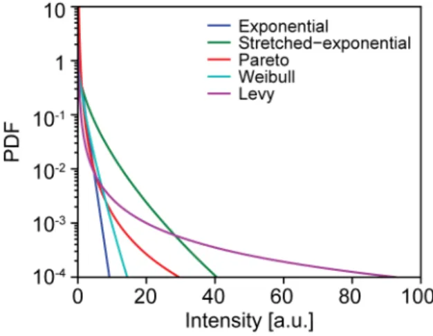
The measurable quantity in optics is the intensity of light. The association of rogue waves with the deviation of field amplitude statistics from Gaussiannity, therefore, often translates into the deviation of intensity probability distribution from an exponential statistics [20, 77–79]. Indeed, the first link between extreme events in nonlinear optics to the one in the ocean is partly due to the experimental observation of ‘L-shaped’ long-tailed distributions, which signifies the non-negligable probability of the extreme events [26]. Following this work, several studies of rogue waves in different optical systems have been done, displaying various types of distributions depending on the system under study [20]. In some works, rogue events are associated with particular extreme-value probability distributions, such as Weibull [80–83], Pareto [80, 83], Log-normal [57], or stretched-exponential distribution [5, 33, 77, 84]. Fig. 2.4 contrasts the long tail property of these distributions to an exponential distribution.

Figure 2.4: Examples of heavy-tailed distributions commonly reported in the study of optical rogue waves, compared to an exponential distribution.

In other cases, however, a particular probability distribution might not be identified due to the complexity of the system, or the statistical approach taken. Therefore, in general, optical rogue wave phenomena are linked with a class long-tailed distribution (for example in Ref. [32, 85–89]) or heavy-tailed distribution (for example in Ref. [28, 57, 78, 81–83, 90–93]). Although sometimes

used interchangably, it is important to note that these distributions do not actually have the same signification. Heavy-tailed is defined as distributions with heavier-than-exponential tails [12]. It is a general term referring to probability distribution function that descends slower than exponential function, which signifies a more probable realisation of extreme values than in a normal distribution. Whilst long-tailed is defined as distributions whose tails are asymptotically self-similar under shifting by a constant, and is a subclass of heavy-tailed distribution [94].

2.2.2 Classification of extreme events as rogue waves

Different simplified criteria in defining oceanic rogue waves have been proposed in the literature. A pragmatic approach is to call a wave a rogue wave whenever the wave height H or the crest height ⌘c exceeds a certain threshold related to the sea state, called the significant wave height (SWH)

HS. In the literature, SWH is commonly defined either as the average of the largest one third of

wave heights H1/3[56], or as four times the standard deviation of the surface elevation. In general

H1/3turns to be approximately 4 , although it has been shown that the results could be different

(H1/3 is typically 5% 10% lower than the value of 4 ) [73, 95]. Since standard deviation is the

fundamental quantity used in oceanography, the definition of SWH as 4 is preferred instead of the original definition in most of recent studies of oceanic rogue waves [14, 17, 20]. Subsequently, following one of these definitions, a rogue wave is defined commonly as a wave with wave height H > 2HSand/or crest height ⌘c> 1.25HS, or both [96]. These simplistic criteria have been argued

however, to be not sufficient as they do not take into account the nature (state) of the sea in which the waves occur [97].

Apart from the rogue threshold criteria, the kurtosis (fourth order statistical moment) of the distribution has also been suggested to be a suitable parameter for the identification of rogue waves in a short-term wave record [98–100]. Indeed, kurtosis is a parameter that measures the heaviness of the tail of the distribution [101], which is related to the probability of rogue wave occurrence.

Similarly, rogue waves in optics have also been identified in a number of different ways. One approach is to associate rogue events with particular extreme-value probability distributions, where such functions have been shown to provide good fits to the tails of optical intensity fluctuation histograms [30, 80, 81]. Another approach adapts one of the oceanographic definition of a rogue wave, where rogue wave height is defined as HRW? 2H1/3. The accessible data in optics however,

is not the field amplitude but rather the intensity, and such data can take a variety of forms: an intensity time series, the levels of a two-dimensional camera image, or the space–time intensity evolution of an optical field. The oceanographic definition of rogue waves is therefore often modified to define a threshold IRW? 2I1/3, where the ‘significant intensity’ I1/3is the mean intensity of the

highest third of events. This definition, although somewhat arbitrary, has been applied in several studies [83, 86, 102, 103].

2.3 Oceanic rogue waves

In recent years, considerable interest in understanding the origin of oceanic rogue waves has led to the development of various physical models to explain their generating mechanisms. Apart from its practical significance to engineers and naval architects, the study of the origin of oceanic rogue

waves is also useful as guidance in setting up different kind of laboratory experiments in related studies. In this section we review the generation of oceanic rogue waves from linear and nonlinear effects, where we focus only on the generation of oceanic rogue waves in the deep water (open sea).

2.3.1 Linear mechanisms

A random sea can be regarded as the result of wave superposition of an infinite number of small amplitude linear waves with different wave amplitudes and frequencies traveling in different directions

⌘(x, t) =X

k

a(k) cos(k.x !t + ↵(k)), (2.1) where ⌘ is the elevation, x is a position vector, and t is the time. The wave number k = |k| and the frequency ! satisfy the dispersion relation

!2_{= gk tanh(hk), (2.2)}

where g is the gravitational acceleration and h is the water depth. The amplitude a and phase ↵ are random variables, uncorrelated for each k.

In the deep water regime, h , tanh(kh) ⇠ 1, and the dispersion relation can be written as ! =pgk. (2.3) Since the relationship between ! and k is not linear, this implies that deep water waves are dispersive, with phase velocity vph

vph= ! k = r g k = g ! (2.4)

and group velocity vgr

vgr= d!_dk = 1 2 r g k = g 2! = vph 2 . (2.5) From here we can see that both the phase velocity and the group velocity are dependent on the frequency (wavelength), where longer waves travel faster.

Spatial / geometrical focussing (spatial caustics)

Geometrical focussing is a well known local amplification process for waves of any physical nature and is related to spatial variation of wave fronts. In the simplest case, a wave front with cylindrical curvature is known to focus into one point. When the curvature of the wave front is complex, however, the focussing may result in spatially distributed focussing areas known as caustics. These caustics can then be considered as rogue waves when the condition described in Section 2.2 is fulfilled.

The curvature of wave front can be modified by the variation of water depth h, as described by the dispersion relation shown in Eq. 2.2. However, this situation is only relevant in the formation of rogue waves in shallow water (coastal zone). In deep water, geometrical focussing can result

from inhomogeneous wind flow (also known as “crossing sea”, see Fig. 2.5(a)) and atmospheric pressure in storm areas, or from the wave interaction with variable currents [13, 14, 16]. Indeed, rogue waves have been observed very often in strong currents, for example in the Agulhas current that passes along the South African coast, suggesting that giant waves are produced by refraction of waves into a caustic region [104–106].

Figure 2.5: (a) Crossing sea, superposition of two wave systems travelling at different directions. (b) Study of wave energy density in a random refracting field for an initial set of parallel rays corresponding to a single plane wave: (i) The random velocity field acting as random refracting medium (darker shades indicate higher velocity); (ii) The focussing of uniform plane wave passing through the random refracting medium from top to bottom (darker areas correspond to higher energy density). Source: from Ref. [4].

Furthermore, it is also pointed out that even small random current fluctuations can result in focussing provided their scale is sufficiently large (on the order of 10 km), as shown in Fig. 2.5(b) [4, 62, 107]. Consequently, the sensitivity of caustics to the small variation of the initial conditions, results in the appearance and disappearance of the focuses at “random” points and “random” times, explaining the rare and short-lived character of the rogue wave phenomenon [13]. Additionally, under hypotheses that the mean current is constant and the random current fluctuations are small, the probability distribution for the formation of the freak waves is shown to be dependent only on the distance scale parameter, independent of the details of the current distribution [62].

Spatio-temporal focussing (dispersive focussing / space-time caustics)

The effect of geometrical focussing in deep water is significant, but the effect of temporal focussing also needs to be taken into account [16]. As we have seen earlier, deep water waves are dispersive with phase and group velocities inversely proportional to the frequency (Eq. 2.4 and 2.5), and may travel along different directions. Consequently, the locations of caustics are frequency-dependent and rogue waves are formed from space-time caustics [108]. Rare extreme wave events can therefore be interpreted as the local intercrossing of a large number of monochromatic waves with appropriate phases and directions [13].

For unidirectional surface waves, it can be understood that when long waves overtake short waves due to dispersion, large-amplitude waves can appear at some fixed time owing to the superposition of all the waves located at the same place, and then the long waves will be in front

of the short waves, forming a short “life time” freak wave. The formation of space-time caustics has been demonstrated in water wave tanks [109]. The idea is to create a long wave group with a properly designed chirp (linearly decreasing frequency) such that it will contract at a given position (to a few wavelengths) as the effect of dispersion.

In two-dimensional space, space-time caustics are formed by the combination of both dispersion and spatial focussing. It has been proposed that although the exact time and location of the wave focussing events are unpredictable, the expected spatio-temporal structure of the wave field in the vicinity of such events is largely predictable [108]. When superimposed with a random-wave field, this dispersion focussing effect will then only be apparent when the amplitude of the chirped wave train is higher than the standard deviation of the surface elevation [14].

It is important to note that although the physical mechanisms that produce the contrived phase relations and chirped wave trains have not been confirmed [14], it is suggested that this rare circumstance can be generated for example by the increase of wind speed that yields the generation of short waves followed by longer waves [15].

2.3.2 Nonlinear mechanisms

Linear theory is based on the assumption that the wave components are harmonic and independent from each other. When the waves are too steep however, the linear wave theory is no longer valid and nonlinear contribution becomes significant. In contrast to the linear theory, nonlinear wave interaction facilitates the exchange of wave energy between different wave components. This implies that random wave background might act on propagating coherent waves (uniform waves), leading to instability of the amplitude modulation of the waves. The effect of nonlinearity in rogue wave formation is therefore actively studied, where it is often associated to the increase in rogue wave probability beyond the conventional linear (or quasi-linear) theories, corresponding to a longer tail in the distribution [20].

Weakly nonlinear waves and the NLSE

Weakly nonlinear theory has been widely suggested to explain the emergence of rogue waves [98]. In general, the degree of wave nonlinearity regardless of the water depth can be measured in terms of a dimensionless parameter known as the wave steepness s = kH/2, where k is the wave number of the carrier wave and H is the wave height. Typical intense ocean wave trains are characterised by the steepness s ⇡ 0.07 0.1. It is known that uniform waves over deep water will grow when the initial steepness is large and then break when reaching a steepness of s ⇡ 0.4 [13, 16, 110]. This phenomenon shows that even though the wave breaking is a strongly nonlinear process, its final effect is to keep the water wave dynamics in a statistically weak nonlinear regime, thus justifying the weakly nonlinear approach [20].

Several reduced mathematical models have been developed for the study of deep-water waves. Among them, the nonlinear Schrödinger equation (NLSE) is often preferred to describe the spontaneous formation of extreme waves “out of nowhere” due to its simplicity and its universality. The NLSE is generic to all conservative systems that are weakly nonlinear and dispersive [111, 112], which was first derived by Zakharov in 1968 [113].