HAL Id: tel-01207252
https://hal.archives-ouvertes.fr/tel-01207252
Submitted on 30 Sep 2015HAL is a multi-disciplinary open access
archive for the deposit and dissemination of sci-entific research documents, whether they are pub-lished or not. The documents may come from teaching and research institutions in France or abroad, or from public or private research centers.
L’archive ouverte pluridisciplinaire HAL, est destinée au dépôt et à la diffusion de documents scientifiques de niveau recherche, publiés ou non, émanant des établissements d’enseignement et de recherche français ou étrangers, des laboratoires publics ou privés.
Unsteady Navier-Stokes Equations
Guang Tao Xu
To cite this version:
Guang Tao Xu. Some advances in PGD-based Model Reduction for High order PDEs, Complex Geometries and Solution of the Unsteady Navier-Stokes Equations . Fluid mechanics [physics.class-ph]. Ecole Centrale de Nantes (ECN), 2014. English. �tel-01207252�
Ecole Centrale de Nantes
Ecole Doctorale
Sciences Pour l’Ingénieur, Géosciences, Architecture
Annèe 2013-2014 N◦B.U :
Thèse de Doctorat
Spècialitè: Mécanique des milieux fluides
Présenté et soutenue publiquement par
Guangtao XU
Le 19 Mai 2014 à L’Ecole Centrale de Nantes
Des avancées dans la réduction de modèle de type PGD
pour les EDPs d’ordre élevé, le traitement des géométries
complexes et la résolution des équations de Navier-Stokes
instationnaires
JURY Rapporteurs:
Cyrille ALLERY Maître de conférences(HDR) - Université de La Rochelle Mejdi AZAIEZ Professeur - Institut Polytechnique de Bordeaux
Examinateurs:
Francisco Chinesta Professeur - Ecole Centrale de Nantes
Christophe Corre Professeur - Institut National Polytechnique de Grenoble Adrien Leygue Chargé de recherche CNRS - Ecole Centrale de Nantes Michel Visonneau Directeur de recherche CNRS - Ecole Centrale de Nantes
Directeur de thèse : Michel Visonneau N◦ED
Laboratoire: Hydrodynamics, Energetics, Atmospheric Environment - Ecole Centrale de Nantes Co-directeur : Francisco Chinesta
Ecole Centrale de Nantes
Ecole Doctorale
Sciences Pour l’Ingénieur, Géosciences, Architecture
Annèe 2013-2014 N◦B.U :
Doctoral Thesis
Subject: Mécanique des milieux fluides
written by
Guangtao XU
defenced on May 19 2014at Ecole Centrale Nantes
Some advances in PGD-based Model Reduction for
High order PDEs, Complex Geometries and
Solution of the Unsteady Navier-Stokes Equations
JURY Reviewers:
Cyrille ALLERY Maître de conférences(HDR) - Université de La Rochelle Mejdi AZAIEZ Professeur - Institut Polytechnique de Bordeaux
Examinators:
Francisco Chinesta Professeur - Ecole Centrale de Nantes
Christophe Corre Professeur - Institut National Polytechnique de Grenoble Adrien Leygue Chargé de recherche CNRS - Ecole Centrale de Nantes Michel Visonneau Directeur de recherche CNRS - Ecole Centrale de Nantes
Thesis supervisor : Michel Visonneau N◦ED
Laboratory: Hydrodynamics, Energetics, Atmospheric Environment - Ecole Centrale Nantes Co-supervisor : Francisco Chinesta
Résumé
L’objectif principal de ce travail est de proposer une nouvelle approche de simulation basée sur une Méthode de réduction du modèle (MOR) utilisant une décomposition PGD. Dans ce travail, cette approche est d’abord utilisée pour résoudre des équations aux dérivées partielles d’ordre élevé avec un exemple numérique pour les équations aux dérivées partielles du quatrième ordre sur le problème de la cavité entraînée. Ensuite un changement de coordonnées pour transformer le domaine physique complexe en un domaine de calcul simple est étudié, ce qui conduit à étendre la méthode PGD au traitement de certaines géométries complexes. Divers exemples numériques pour différents types de domaines géométriques sont ainsi traités avec l’approche PGD.
Enfin, une séparation espace-temps est proposée pour résoudre les équations de Navier-Stokes instationnaires à l’aide d’une approche PGD. Cette décomposition est basée sur le choix de modes temporels communs pour la vitesse et la pression, ce qui conduit à une décomposition basée sur des modes spatiaux satisfaisant in-dividuellement la condition d’incompressibilité. L’adaptation d’une formulation volumes finis à cette décomposition PGD est présentée et validée sur de premiers exemples analytiques ou académiques pour les équations de Stokes ou Navier-Stokes instationnaires. Une importante réduction des temps calculs est observée sur les premiers exemples traités.
Mots clés:
Réduction de modèles; PGD; géométrie complexe; EDP d’ordre élevé; Navier-Stokes instationnaire, solveur ISIS-CFD.
Abstract
The main purpose of this work is to describe a simulation method for the use of a PGD-based Model reduction Method (MOR) for solving high order partial differential equations. First, the PGD method is used for solving fourth order PDEs and the algorithm is illustrated on a lid-driven cavity problem. Transformations of coordinates for changing the complex physical domain into the simple computational domain are also studied, which lead to extend the spatial PGD method to complex geometry domains. Some numerical examples for different kinds of domain are treated to illustrate the potentialities of this methodology.
Finally, a PGD-based space-time separation is introduced to solve the unsteady Stokes or Navier-Stokes equations. This decomposition makes use of common tem-poral modes for both velocity and pressure, which lead to velocity spatial modes satisfying individually the incompressibility condition. The adaptation and imple-mentation of a PGD approach into a general purpose finite volume framework is described and illustrated on several analytic and academic flow examples. A large reduction of the computational cost is observed on most of the treated examples.
Keywords:
Reduced Order Models; PGD method; Complex geometry; high order PDEs; Unsteady Navier-Stokes Equations; ISIS-CFD solver.
Contents
List of figures ix
General Introduction 1
I PGD for the High order PDEs, Complex Geometry problem 5
1 High Order PDEs and Complex Geometry problem 7
1.1 High Order PDEs . . . 7
1.2 Complex Geometry domain . . . 9
1.3 Model Reduction Method . . . 11
1.4 Scope and Outline for Part I . . . 12
2 PGD for High order PDEs Problem 15 2.1 Introduction . . . 16
2.1.1 Harmonic problem and Biharmonic problem . . . 16
2.1.2 Chebyshev polynomials & Chebyshev method . . . 17
2.1.3 Numerical results . . . 20
2.1.4 2D incompressible Flow problem . . . 23
2.2 PGD formulation for High order PDEs . . . 25
2.2.2 Pseudo-Spectral Chebyshev method . . . 28
2.3 Numerical results . . . 30
2.3.1 2D Laplace problem . . . 30
2.3.2 4th order PDE problem . . . 31
2.3.3 Chebyshev Polynomials for Boundary Value Problem . . . 35
2.3.4 PGD for the Non-Homogeneous BC Biharmonic Problem . . . 47
2.3.5 PGD method for the Lid driven cavity problem . . . 48
2.4 Discussion and Conclusion . . . 52
3 PGD for the Decomposition of Complex Geometry 55 3.1 Introduction . . . 55
3.1.1 Coordinate transform for Complex Geometry . . . 56
3.1.2 FD method in the (θ, r) variables . . . 58
3.1.3 Examples for the different kinds of domain . . . 59
3.2 PGD applied to a complex geometry problem . . . 63
3.2.1 General weak form for the new formulation . . . 63
3.3 Numerical examples. . . 68
3.3.1 Manufactured problem . . . 69
3.3.2 Circular Domain with Uniform Source Term . . . 71
3.3.3 Circular Domain with Non-uniform Source Term. . . 71
3.3.4 Ellipsoidal Domain . . . 74
3.3.5 Star Domain. . . 77
Contents
II PGD for Resolving the Unsteady Navier-Stokes Equations 81
4 Resolving the Unsteady Navier-Stokes Equations 83
4.1 Fluid flow and Navier-Stokes Equations . . . 83
4.2 Numerical Method for the Navier-Stokes Equation . . . 85
4.3 Model Reduction Method . . . 88
4.4 Scope and Outline of Part II . . . 89
5 The ISIS-CFD flow solver 91 5.1 Introduction . . . 91
5.2 The ISIS-CFD flow solver . . . 92
5.2.1 Reynolds Averaged Navier-Stokes Equations . . . 92
5.2.2 Discretization of the momentum equation . . . 92
5.2.3 Velocity-pressure coupling algorithm . . . 94
5.2.4 The linear solvers . . . 96
5.3 Numerical results . . . 97
5.3.1 Steady Stokes for Lid driven cavity . . . 97
5.3.2 Analytical solution for Steady Stokes . . . 101
5.4 Discussion and Conclusion . . . 104
6 PGD for Resolving the Unsteady Navier-Stokes Equations 105 6.1 Introduction . . . 106
6.2 Singular Value Decomposition (SVD) for ISIS-CFD solution . . . 106
6.2.1 Singular Value Decomposition (SVD) . . . 106
6.2.2 Numerical example for SVD of ISIS-CFD solution . . . 107
6.3 The PGD algorithm illustrated on an unsteady convection-diffusion equation . . . 116
6.3.1 Computing the function S(x) . . . 117
6.3.2 Computing the function R(t) . . . 117
6.4 Comparison between an incremental approach and a separated decom-position . . . 118
6.4.1 In terms of computational effort . . . 118
6.4.2 In terms of memory allocation . . . 119
6.5 PGD formulation for Resolving the Unsteady Navier-Stokes equations 119 6.5.1 Introduction . . . 119
6.5.2 Unsteady Stokes Equations . . . 120
6.5.3 PGD Generalization to the unsteady 2D Stokes equations for incompressible flows . . . 120
6.5.4 A pressure equation formulation to solve the PGD formulation of Navier-Stokes equations for incompressible flows . . . 124
6.6 Treatment of non-linearities for the Navier-Stokes equations . . . 127
6.6.1 Linearization of the non-linear terms in the Navier-Stokes. . . 129
6.6.2 PGD formulation for the linearization . . . 130
6.6.3 Simplifying more the linearization . . . 137
6.7 Discussion and Conclusion . . . 139
7 Application of PGD for solving Unsteady Navier-Stokes equations141 7.1 Introduction . . . 141
7.2 Analytical flow problems . . . 142
7.2.1 Unsteady Diffusion problem . . . 142
7.2.2 Analytical Stokes problem . . . 145
7.2.3 Burgers problem . . . 149
7.3 Real flow problem . . . 153
Contents
7.3.2 Navier-Stokes flow in a lid-driven cavity . . . 157
7.3.3 2D Couette flow. . . 161
7.4 Discussion and Conclusion . . . 163
Conclusions and Perspectives 165
List of Figures
2.1 Graphic of the Chebyshev polynomials for k = 0, · · · , 6 . . . 18
2.2 Laplace solution and Convergence . . . 21
2.3 Exact solution and Chebyshev solution for 4th order problem. . . 22
2.4 Error between the exact solution and Chebyshev solution . . . 22
2.5 The contour for the 2D Stokes problem . . . 23
2.6 Singular values and finite sum representation for the flow problem . . 24
2.7 Error between the finite sum with 10 terms and the solution . . . 24
2.8 Result for laplace problem . . . 31
2.9 PGD modes and PGD convergence . . . 31
2.10 Error for PGD and FD solution compare with exact solution . . . 32
2.11 L − 2 Error for PGD and Exact solution VS PGD modes . . . 32
2.12 Exact solution and PGD solution . . . 33
2.13 PGD mode and PGD convergence . . . 33
2.14 Error between the PGD solution and exact solution . . . 34
2.15 CPU time and L2 error compare between the 2-D Chebyshev method and PGD method . . . 35
2.16 Test case 1 . . . 37
2.17 Test Case 2 . . . 38
2.19 Result from Chebyshev Polynomials for Boundary Value Problem . . 42
2.20 Geometry and Boundary Condition for the 2D problem . . . 43
2.21 The solution from chebyshev method . . . 45
2.22 Souce term . . . 46
2.23 Error for the Lid driven cavity problem . . . 49
2.24 Contour by PGD and the Chebyshev method . . . 50
2.25 PGD modes and PGD convergence . . . 50
2.26 Error for the Lid driven cavity problem . . . 51
2.27 Contour by PGD and the Chebyshev method . . . 51
2.28 PGD convergence . . . 52
3.1 Complex Geometry domain . . . 56
3.2 Solution for unit Circle domain . . . 60
3.3 Solution for Slanted Ellipse domain . . . 60
3.4 Mesh for the star domain . . . 61
3.5 a(θ), b(θ), c(θ), d(θ) for the star domain . . . 61
3.6 FE mesh and FE solution . . . 62
3.7 FD solution and FD-FE comparison . . . 62
3.8 Solution for the square domain . . . 62
3.9 Solution for the manufactured problem . . . 70
3.10 Error for the manufactured problem . . . 70
3.11 PGD convergence . . . 71
3.12 PGD solution for the circular domain . . . 72
3.13 PGD error for the circular domain. . . 72
3.14 PGD convergence for the circular domain . . . 72
List of Figures
3.16 PGD error for the problem with Non-uniform Source . . . 73
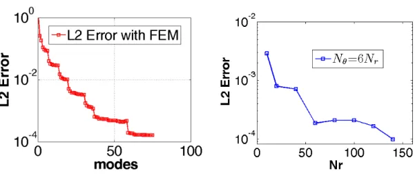
3.17 PGD error as a function of the number of modes and Error of the converged PGD solution (the discretization for (θ, r) have the relation Ntheta= 6Nr) for the the problem with Non-uniform Source . . . 74
3.18 Geometry for the Ellipsoidal domain . . . 75
3.19 Solution for the Ellipsoidal domain . . . 75
3.20 PGD error for the Ellipsoidal domain . . . 76
3.21 PGD Convergence and Error of the converged PGD for different meshes for the Ellipsoidal domain . . . 76
3.22 Comparison of CPU time between PGD and FEM . . . 76
3.23 Geometry for the Star Domain . . . 77
3.24 Solution for the Star Domain . . . 78
3.25 PGD error for the Star Domain compare with the FEM solution . . . 78
3.26 PGD convergence and PGD-FEM error for different meshes for the star domain . . . 79
3.27 FEM-PGD CPU time comparison for the star-like domain. . . 79
4.1 Flow around submarine . . . 84
4.2 Flow generated by an earthquake . . . 84
4.3 The flow from a faucet . . . 85
4.4 Comparison of the PGD and FEM based 3D discretizations . . . 89
4.5 CPU time for the PGD and standard solvers . . . 89
5.1 Geometry and boundary conditions for the lid driven cavity . . . 98
5.2 Convergence analysis . . . 99
5.3 FV and FE solutions for Lid-driven cavity . . . 99
5.4 FEM and FVM solutions for the lid-driven cavity (streamlines). . . . 100
5.6 Residual vs number of nodes for 4 cases. . . 102
5.7 Evolution of the CPU time and number of iterations to converge for various grids . . . 102
5.8 L-2 norm of error for the velocities and pressure . . . 103
6.1 Geometry and boundary conditions . . . 108
6.2 3rd mode for u . . . 109
6.3 4th mode for u . . . 110
6.4 Eigenvalue for U . . . 110
6.5 Error for U (logplot) . . . 110
6.6 1st-3rd modes for v . . . 112
6.7 4th mode for v . . . 113
6.8 Eigenvalue for V . . . 113
6.9 Error for V (logplot) . . . 113
6.10 1st-3rd modes for P . . . 114
6.11 4th mode for Pressure . . . 115
6.12 Eigenvalue for Pressure . . . 115
6.13 Error for Pressure (logplot) . . . 115
7.1 PGD solution (top) & error with analytical solution (bottom) at 0.01s143 7.2 PGD solution (top) & error with analytical solution (bottom) at 0.2s 143 7.3 PGD solution (top) & error with analytical solution (bottom) at 0.9s 144 7.4 Space and time discretization effects for the diffusion problem . . . . 144
7.5 Convergence for the diffusion problem . . . 145
7.6 Geometry and boundary conditions for the Stokes analytical flow . . 146
7.7 PGD solution (top) & exact solution (bottom) at 0.01s . . . 147
List of Figures
7.9 PGD solution (top) & exact solution (bottom) at 0.9s . . . 148
7.10 Space and time discretization effect for the analytical Stokes problem 148 7.11 Convergence for the analytical Stokes problem . . . 149
7.12 Geometry and boundaries for Burgers equation . . . 149
7.13 PGD solution for Burgers equation at 0.01s . . . 151
7.14 PGD solution for Burgers equation at 0.2s . . . 151
7.15 PGD solution for Burgers equation at 0.9s . . . 152
7.16 Error vs PGD modes for Burgers equation . . . 152
7.17 Space and time discretization effects for Burgers equation . . . 153
7.18 Geometry and boundary conditions for the lid-driven cavity flow . . . 154
7.19 PGD solution at 0.01s for the lid-driven cavity problem . . . 155
7.20 PGD solution at 0.2s for the lid-driven cavity problem . . . 156
7.21 PGD solution at 0.9s for the lid-driven cavity problem . . . 156
7.22 Convergence for the lid-driven cavity problem . . . 157
7.23 CPU time comparison for the lid-driven cavity problem . . . 157
7.24 PGD solution with 20 modes and the ISIS-CFD solution for the lid-driven cavity problem by Navier-Stokes (continuous line: ISIS-CFD solution, dashed line: ISIS-CFD-PGD solution) . . . 158
7.25 PGD solution with 50 modes and the ISIS-CFD solution for the lid-driven cavity problem by Navier-Stokes ((continuous line: ISIS-CFD solution, dashed line: ISIS-CFD-PGD solution) . . . 159
7.26 PGD convergence vs modes number . . . 160
7.27 CPU comparison for the lid-driven cavity . . . 160
7.28 Geometry for the Couette flow problem . . . 161
7.29 PGD solution with 20 modes and the ISIS-CFD solution (continuous line is ISIS-CFD solution and dashed line is ISIS-CFD-PGD solution) 162
7.30 PGD solution with 32 modes and the ISIS-CFD solution(continuous line is ISIS-CFD solution and dashed line is ISIS-CFD-PGD solution) 162
7.31 L − 2 norm of the difference for U, p vs modes number . . . 163
General Introduction
Model reduction Method is the calculation of the problem in the science and the engineering for the complex geometry problem and with their thermo mechanical behavior. Many of them have never been solved because of the computational complexity caused by such problems. This method can be very fast for these problem, which are real time solving for some problem.
Along with the ROM-POD method[Kerschen et al., 2005,Liberge, 2010] and the reduced-basis element method [Rozza et al., 2008], Proper general decomposition (PGD) method is one kind of Model reduction Method (MOR) which is a kind of very efficient method to solve the multi phase problem, but in the case of PGD the construction of the representation takes into account the nature of the problem directly. The general form of a PGD separated representation of a function u of N variables is
u(x1, ..., xN) =PMm=1u1m(x1) × ... × uNm(xN), M being the order of the approximation.
This method is based on the space-time separated idea, but this idea is not a new proposal. In fact, it was proposed by Pierre ladeveze as an ingredient of new powerful non-linear non-incremental LATIN solver in the 80s. In the LATIN method, radial approximation are used as a approach which could be seen as a variation of the PGD with a space-time separation (see example as [Ladevèze, 1999, Ladevèze et al., 2010, Ladevèze and Nouy, 2003, Cremonesi et al., 2013]). And PGD now has been used to solve many kinds of problem in multi-dimensional spaces: quantum chemistry, kinetic theory description of complex fluid and chemical master equations, etc...The interested reader can refer to [Chinesta et al., 2011] for a recent review in the context of computational rheology.
Many problems governed by multi-harmonic equations, such as thin-plate bending and Stokes flow problems which involve biharmonic equations. And many real engineering problem are concerned with the problem in the complex geometry. But no work has been done by the PGD based Model reduction Method (MOR) for high order PDEs problem, even fewer works has been done for the problem with complex geometry which is always concerned by the real engineering problem. In this work, the PGD method for solving the high order PDEs problem and the problem with
complex geometry domain are proposed in the first part.
In the Chapter 1, the state of the art for the high order PDEs problem and the problem in complex geometry domain is presented, and the PGD based MOR will introduced and the progress for this kind of MOR will be presented.
Secondly, after the common method -Chebyshev method for solving the high order PDEs is introduced, the PGD method for solving the high order PDEs is presented in the Chapter 2, the numerical example for the fourth order PDEs and Lid driven cavity problem will be detailed.
At last of the first part, transformation of coordinates for changing the complex domain problem into the simple compute domain will be studied in the Chapter 3, then the PGD method for the complex geometry problem is proposed in the same chapter, the numerical examples for different kinds of domain problem are resolved by the PGD method.
In the other part, because of the nonlinear terms, convective terms and the pressure gradient term, it is very difficulty for solving the Navier-Stokes equations, more transient resolutions need a small enough time step to ensure the stability and convergence of numerical schemes. so it is desirable to have a sufficient density of points to describe the interface of discontinuity. There were a lot of problems related to the very large calculations [Montagnier et al., 2013]. Efficient solver are needed for the simulation. Although the PGD based Model reduction Method (MOR) has been done in some work for resolving the Navier-stokes problem, but never been done with the real kind of Navier-stokes equations. So, in the second part, we will use PGD method for Resolving the Unsteady Navier-Stokes Equations, apply the model reduction techniques based on the method PGD (Proper Generalized Decomposition) for non-incremental discretization of the Navier Stokes equations.
The Chapter 4 will make a point on the vast state of art on Navier-Stokes Equation and numerical methods for solving the Navier-stokes Equations, and also the Proper Generalized Decomposition Methods for solving the flow problem will be stated.
The Chapter 5 will present the basic theory for the ISIS-CFD solver [Deng et al., 2001,Queutey and Visonneau, 2007] and a numerical example will be presented for solving the steady stokes in the lid driven cavity problem.
The Chapter 6 will firstly use the SVD for representing the unsteady flow by the priori solution from the ISIS-CFD solver of the 2D unsteady flow in lid-driven cavity. Then we will give the theories about the PGD method coupling with the ISIS-CFD solver for the Unsteady Navier-Stokes Equations without the nonlinear
General Introduction
term; the same temporal function for the velocity and pressure for the decomposition is used, this strategy was used for avoiding to change the incompressible problem into the compressible problem. The finite volume formulation for the PGD method for solving the unsteady Reynolds Averaged Navier-Stokes Equation will also be given in this chapter.
The numerical examples for using the proposed PGD method to the flow problems governed by STOKES and Navier-stokes equations will be given in the Chapter 7.
Part I
PGD for the High order PDEs,
Complex Geometry problem
Chapter 1
High Order PDEs and Complex
Geometry problem
1.1 High Order PDEs . . . . 7
1.2 Complex Geometry domain . . . . 9
1.3 Model Reduction Method . . . . 11
1.4 Scope and Outline for Part I . . . . 12
1.1
High Order PDEs
Partial differential equations (PDEs) defined on surfaces embedded in R3 arise in a wide range of applications [Greer et al., 2006], including fluid dynamics, biology (e.g., fluids on the lungs), materials science (e.g., ice formation), electromagnetism, image processing (e.g., images on manifolds and inverse problems such as EEG), computer graphics (e.g., water flowing on a surface), computer aided geometric design (e.g., special curves on surfaces), and pattern formation. Alternating Direction Implicit (ADI) schemes are constructed for the solution of two-dimensional higher-order linear and nonlinear diffusion equations, particularly including the fourth-order thin film equation for surface tension driven fluid flows [Witelski and Bowen, 2003]. In [Mai-Duy and Tanner, 2005], the unsymmetric indirect RBF collocation method is extended to solve high-order PDEs directly, and the method is verified successfully through the solution of thin-plate bending and viscous flow problems which are governed by biharmonic equations.
bending and Stokes flow problems involving biharmonic equations. The Biharmonic problem [Erturk and Dursun, 2007] which is a 4-th order PDEs problem has been raised in many research filed, such as in elasticity problem which dealing with the transverse displacements of plates [Li et al., 2011] and shells and in fluid problem which the governing equation of the stokes flow [Montlaur et al., 2008] is the bihar-monic equation. In the thin plate theory, the biharbihar-monic equation can be represent the clamped plate under the external load [Li et al., 2011]. As we know, the bound-ary and load condition is very complex, so it’s very difficulty to get the analytical solution. Therefore, many studies are focus on the numerical method to make the biharmonic problem to practical engineering.
To solve these problems, new variables are usually introduced in order to transform the multi-harmonic equations into the coupled sets of harmonic equa-tions from which the conventional low-order methods of discretization such as the boundary element methods (BEMs) [Mai-Duy et al., 2006], finite dif-ference methods (FDMs) or finite element methods (FEMs)[Gudi et al., 2008] can be applied for obtaining a numerical solution [Mai-Duy and Tanner, 2005], but the researchers are interested in using the spectral method, such us Variational iteration method [Ali and Raslan, 2007], Domain Decomposi-tion Method [Avudainayagam and Vani, 2000, Shang and He, 2009], finite volume method[Wang, 2004], Fast multiple method [Gumerov and Duraiswami, 2006] and fundamental solutions method [Marin and Lesnic, 2005].
Due to their bigger accuracy when compared to Finite Differences (FD) and Finite Elements (FE) methods, the rate of convergence of spectral approximations depends only on the smoothness of the solution, yielding the ability to achieve high precision with a small number of data. The spectral method has been popularly used in the computation of continuous mechanics problems. The expression spectral methods has different meanings for several sub-areas of Mathematics, like Functional Analysis and Signal Processing, Spectral methods has the meaning of a high accuracy numerical method to solve Partial Differential Equations. The numerical solution is expressed as a finite expansion of some set of basis functions. When the PDE is written in terms of the coefficients of this expansion, the method is known as a Galerkin spectral method. Spectral collocation methods, also known as pseudo spectral methods, is another subclass of spectral methods which are similar to Finite Differences methods due to direct use of a set of grid points, which are called ”collocation points”. A third class are the Tau spectral methods. These methods are similar to the Galerkin spectral methods, however the expanding basis is not obliged to satisfy the boundary conditions, requiring extra equations. In a spectral collocation method based on integrated chebyshev polynomials for the solution of first and second kind of biharmonic problems is analyzed [Mai-Duy and Tanner, 2007].
1.2. Complex Geometry domain
This kind of method has been successfully used to solve the harmonic and biharmonic problem in [Chantasiriwan, 2006].
The Chebyshev spectral collocation method [Martinez and Esperança, 2007, Li et al., 2008] can be described in the following way. An approximation based on Chebyshev polynomials to the variable u is first introduced. The set of collocation equations is then generated. The equation system consists of two parts. The first part is formed by making the associated residual, e.g.(42u − f ), equal to zero at
the collocation points; while the second part is obtained by forcing the boundary conditions e.g., u and au
ax, to be satisfied at the boundary collocation points. These
tasks need to be conducted in an appropriate manner.
1.2
Complex Geometry domain
In the science and engineering problems, many real problems are relevant with the complex geometry domain, for example Shape Optimization [Wang, 2012, Yoon and Sigmund, 2008], not as simple as the rectangular or square domain which can be easily applied the Finite Difference Method for example when the numerical simulation were needed to be done; so for the problem on irregular domains, it is still challenging to solve the partial diffusion equation efficiently.
Currently, the FDM were used for the problem in irregular domain, but the Finite Difference approximation need to be modified at grids near the boundary. Due to the difficulties in handling the finite difference approximation close to a curved boundary, most the finite difference methods are restricted on regular (rect-angular and circular) domains. [Lai, 2001] proposed a simple second-order finite difference treatment of polar coordinate singularity for Poisson equation on a disk; [Chen et al., 2008] has proposed a fast FDM for biharmonic equations on irregular domain. [Weibin and Xionghua, 2009] proposed a meshless method: Chebyshev tau matrix method (CTMM) for Poisson-type equations on irregular domains. The Fast Fourier Transform (FFT) was used to transform from the physical space to the spectral space efficiently and the matrix technique was used to represent the differ-entiation. [Shao et al., 2012] reported the Chebyshev tau meshless method based on the integration differentiation (CTMMID) for numerically solving Biharmonic-type equations on irregularly shaped domains with complex boundary conditions. An integral collocation approach based on Chebyshev polynomials for numerically solving biharmonic equations further developed for the case of irregularly shaped domains in [Mai-Duy and Tran-Cong, 2009]. [McCorquodale et al., 2004] presented a method for solving Poissons equation with Dirichlet boundary conditions on an
three-dimensional irregular bounded region. A pervasive embedded boundary domain specification for the data connected with the numerical integration of conservation-law PDEs was studied by [Day et al., 1998]. [Li et al., 2009] studied a generalized ap-proach for solving the complex, stationary, or moving geometries with Dirichlet, Neu-mann, and Robin boundary conditions Partial Differential Equations. [Mayo, 1984] proposed an the embedded boundary integral method (EBI) for the Poisson’s and the Biharmonic Equations on Irregular Regions, and extended this method to the stokes flow in complex geometry [Biros et al., 2004]. The method for solving fourth order PDEs on surfaces of arbitrary geometry by finite difference schemes on a Cartesian grid was studied by [Greer et al., 2006]. Meshless method were used for solving coupled radiative and conductive problem for the complex geometries in [Sakami et al., 1996, Wang et al., 2010, Sadat et al., 2012].
In the fluid mechanics, one of the main challenges for the Navier-stokes solver is the geometric flexibility, the unstructured grids is not always adopted as the filetering procedure involved in LES and is associated with increased computing cost [Bui, 2000]; simulation results for a variety of flows to show that robust, accurate solutions are now obtained at high Reynolds numbers in very complex geometries in [Mahesh et al., 2004]; In [Münster et al., 2012] explain the details of how the fictitious boundary method (FBM) can be used to simulate flows with complex geometries that are hard to describe analytically, also explained how complex geometry can be easily used in the Finite element-fictitious boundary methods (FEM-FBM) for context. Spectral methods are known to be well suited for laminar or transitional flows in simple geometries (Cartesian, cylindrical, spherical...), [Baur et al., 2009] described some routes allowing to address more complex flows, especially turbulent flows in complex geometries. Solving the time-dependent fluid equations as opposed to the time-averaged equations (as done in most solvers) is significantly more stable because the solution is integrated forward in time from a valid solution. However, this approach is often prohibitive and requires typically an order of magnitude or more increase in computing, as well as robust models for any unresolved scales (subgrid stress models or turbulence models) [Duggleby et al., 2011]. Therefore, the first challenge in reducing the time for a CFD solution is reducing the simulation time [Cant, 2002]. The second challenge in shortening the total time of CFD is meshing. In all CFD, mesh quality plays a significant role in improving both solution convergence as well as accuracy [Lohner, 2007].
Nowadays GMSH is 3D finite element grid generator with a build-in CAD engine and post-processor [Geuzaine and Remacle, 2009], the mesh generator by GMSH is well used in many computed code. DistMesh is a simple MATLAB code for generation of unstructured triangular and tetrahedral meshes [Perssont and Strangt, 2004], but the main disadvantage are slow execution and the possibility of nontermination. It is
1.3. Model Reduction Method
still challenge for finding a fast and easy handling method for generate the mesh for simulation, also the mew method for reducing the simulation time are needed.
1.3
Model Reduction Method
As model reduction is a mathematical theory to find a low-dimensional approximation for a system of ordinary differential equations, model reduction is a topic which receives growing attention, both in the mathematics community and the various application areas. It can be used to reduce the computational effort. It is also has been used to solve the fluid problem, Balanced truncation model reduction methods used to analysis the stokes equation in [Stykel, 2006], the important properties of this method are that the regularity and stability is preserved in the reduced order system and there is a priori bound on the approximation error [Vierendeels et al., 2007] developed reduced order models for strongly coupled fluid-structure interaction problem. This method was used for the fluid and the structural solver that are built up during the coupling iterations. The method also can be implemented very easily. [Buffat et al., 2011] presented a spectral projection method for incompress-ible flow simulation based on an orthogonal decomposition of the velocity into two solenoid vector fields and to apply it for the problem of boundary layer bypass transition in a plane channel configuration. One can see the other model reduction method such as ROM-POD method in [Kerschen et al., 2005, Allery et al., 2005, Burkardt et al., 2006, Liberge, 2010, Allery et al., 2011]and the reduced-basis ele-ment method in [Rozza et al., 2008] and the reference therein.
Another possible strategy able to compute the partial differential equations is proper general decomposition (PGD) method which is a kind of very efficient method to solve the multi phase problem. This method is based on the space-time separated idea, but this idea is not a new proposal. In fact, it was proposed by Pierre ladeveze as an ingredient of new powerful non-liner non-incremental LATIN solver in the 80s. In the LATIN method, radial approximation are used as a ap-proach which could be seen as a variation of the PGD with a space-time separation (see example as [Ladevèze, 1999, Ladevèze et al., 2010, Ladevèze and Nouy, 2003, Cremonesi et al., 2013]). The functions depending on space and the ones depend-ing on time were also unknown, and were computed by a suitable technique. [Ammar et al., 2006, Ammar et al., 2007] proposed the Proper general decompo-sition (PGD), and they used this decompodecompo-sition solved many kind of problem in multidimensional spaces, quantum chemistry, kinetic theory description of com-plex fluide, chemical master equation · · · . A detail review work can be found in [Chinesta et al., 2010b,Chinesta et al., 2013]. In the modeling of polymeric liquids,
which need to solve the Fokker-Planck equation, based on PGD, the case of non-homogeneous flows was analyzed [Mokdad et al., 2010, Pruliere et al., 2008]. The models arising from quantum chemistry, since the equations that govern the electronic distribution, the Schrodiger equation are defined in spaces whose dimensionality scales with the number of elementary particles involved in the quantum system, these models are redoubtable, by using PGD, in many system the real issue could be circumvented [Ammar et al., 2008, Ammar and Chinesta, 2008]. Analyzed the non-liner models by an incremental linearization and a Newton linearization [Ammar et al., 2010d], also in [Ammar et al., 2010a,Pruliere et al., 2010] gave the tensor notation for PGD, in [Ammar et al., 2010b] the enforcement of Non-homogeneous boundary conditions and the treatment of complex geometries were involved; and it was also applied for solving multi-physics models arising in the composites manufacturing processes, where are coupled with the non-linear thermal and thermo-mechanical behaviors [Prulière et al., 2010] . And PGD was also applied to the kinetic theory descrip-tion of complex fluid. Related to parametric deterministic models and models in particular were involved in non-Newtonian fluids [Ammar et al., 2010c]. The direct solution of Fokker-planck equation for complex fluids in configuration spaces of high dimension was given in [Chinesta et al., 2011]. PGD also can be coupled with FEM [Ammar et al., 2010d] and BEM [Bonithon et al., 2011] for solving the partial different equation (PDE), the non-incremental compute strategy which used by PGD method demonstrate that significant CPU time savings are expected and alleviate the storage needs.
PGD with a spectral collocation method to solve transfer equations as well as NavierStokes equations has been done in [Dumon et al., 2013], but nothing has been done with the high order PDEs problems. There were only few PGD works concerned with the complex geometry problem, see example [González et al., 2010, Ghnatios et al., 2012,Ammar et al., 2014,Chady Ghnatios, 2012], more work in the complex geometry problem are need to be done.
1.4
Scope and Outline for Part I
The objective of this part is the application of model reduction techniques based on the method PGD (Proper Generalized Decomposition) for solving the high PDEs problem and the problem in complex geometry domain. The oeuvre is developed in the following way:
• The Chapter2will introduce the Chebyshev method for solving the fourth-order PDEs which can be used for the flow streamline. The PGD method was coupling
1.4. Scope and Outline for Part I
with the spectral discretization method for the fourth order PDE. And using the PGD for solving the high order PDEs problem, especially for the 2D lid driven cavity flow problem.
• The Chapter 3will change the equation in the complex geometry problem into the rectangular compute domain by using the coordinate transformation; then we apply PGD to the problem in the complex geometric domain, and several examples with different kind of shape function are applied by the proposed PGD method.
Chapter 2
PGD for High order PDEs
Problem
2.1 Introduction . . . . 16
2.1.1 Harmonic problem and Biharmonic problem. . . 16
2.1.2 Chebyshev polynomials & Chebyshev method . . . 17
2.1.3 Numerical results . . . 20
2.1.4 2D incompressible Flow problem . . . 23 2.2 PGD formulation for High order PDEs . . . . 25
2.2.1 Coupling PGD and Chebyshev method . . . 25
2.2.2 Pseudo-Spectral Chebyshev method . . . 28 2.3 Numerical results . . . . 30
2.3.1 2D Laplace problem . . . 30
2.3.2 4th order PDE problem . . . 31
2.3.3 Chebyshev Polynomials for Boundary Value Problem. . . 35
2.3.4 PGD for the Non-Homogeneous BC Biharmonic Problem . . . 47
2.3.5 PGD method for the Lid driven cavity problem . . . 48 2.4 Discussion and Conclusion . . . . 52
Equations of the harmonic and biharmonic types are two kinds of equation frequently encountered in engineering problems: the biharmonic equation with a given Boundary Condition can be used to describe the stream function for incompressible flow problems for example. Concerning solution strategies, the Pseudo-Spectral Chebyshev method which is based on integrated Chebyshev polynomials for the solution of the problem has been popularly used in the solution of continuous mechanics problems. In this chapter, we propose a technique that combines the use
of Pseudo-Spectral Chebyshev method with the Proper Generalized Decomposition (PGD) that allows space time separated representation of the unknown field within a non incremental integration scheme. We have used the PGD to separate the unknown field between the different coordinates, then Pseudo-Spectral Chebyshev method is used to solve the resulting one dimension problems. We proposed the technique to solve the harmonic problem and the fourth order PDE–biharmonic problem. Specific strategies for dealing with non-homogeneous boundary conditions have been implemented to solve the lid-driven cavity problem in the stream function formulation.
This chapter is thus organized as follows:
First, we give some introduction about the Chebyshev method and describe the harmonic problem and biharmonic problems which are used in this chapter. A 2D Chebyshev method is used for the flow problem and the SVD is used for studying the separability of the 2D solution. In Section 2 we couple the PGD method and the Chebyshev method for the harmonic and biharmonic problem, we considered Pseudo-Spectral Chebyshev method for solving the different one dimensional problems. Section 3 is concerned with applications and numerical examples using the method. A significant part of the section is dedicated to the discussion of different techniques for the imposition of non-homogeneous boundary conditions within the Chebyshev-PGD framework. Finally, Chebyshev-PGD method was applied to the Non-Homogeneous Biharmonic Problem and the proposed technique was used to solve the lid-driven cavity problem in the stream function formulation.
2.1
Introduction
2.1.1 Harmonic problem and Biharmonic problem 2.1.1.1 2D Harmonic problem
The harmonic problem, found in the Laplace equation and Poisson equation, is overwhelmingly present in PDEs describing physical problems and is often a standard benchmark to test the program code.
We consider the problem:
∆u = h(x, y) in Ω (2.1)
with boundary condition:
2.1. Introduction
where ∆ is the Laplace operator, g is a given function, Ω is a bounded domain in the plane, and ∂Ω is the boundary of the domain.
2.1.1.2 2D Biharmonic problem
The Biharmonic problem [Erturk and Dursun, 2007] has been raised in many research fields, such as in elasticity problem which deal with the transverse displacements of plates [Li et al., 2011] and shells as well as in fluid problem where the governing equation for the stokes flow in stream function formulation [Montlaur et al., 2008] is the biharmonic equation. In the thin plate theory, the biharmonic equation can model a clamped plate under some external load [Li et al., 2011].
Here, we consider the Biharmonic problem which follows:
42u = f (x, y) in Ω (2.3) u = 0 and ∂u ∂n = 0 on ∂Ω (2.4) where 42 = ∂4 ∂x4 + 2 ∂4 ∂x2∂y2 + ∂4 ∂y4 (2.5)
and f is a given function.
2.1.2 Chebyshev polynomials & Chebyshev method
The Chebyshev Spectral Collocation method for a differential problem [Martinez and Esperança, 2007, Li et al., 2008] can be described in the following way. An approximation based on Chebyshev polynomials of the unknown function u is first introduced. The set of collocation equations is then generated. The equation system consists of two parts. The first part is formed by making the associated residual, e.g.(42u − f ), equal to zero at the collocation points, while the second part
is obtained by enforcing the boundary conditions e.g., and au
ax , to be satisfied at the
boundary collocation points. These tasks need to be conducted in an appropriate manner and they will be presented in detail.
It is convenient for the Chebyshev method to select the interpolation points in the interval [−1, 1]
xj = cos
πj
The Chebyshev polynomial of the first kind Tk(x) with the polynomial of degree k defined for x ∈ [−1, 1] by Tk(x) = cos(k cos−1x)) (2.7) which − 1 ≤ Tk(x) ≤ 1 (2.8) It is straightforward to deduce: T0(x) = 1 T1(x) = x T2(x) = 2x2 − 1 (2.9)
the Chebyshev polynomials for k = 0, · · · , 6 are represented in Figure (2.1).
−1 −0.5 0 0.5 1 −1 −0.5 0 0.5 1
x
Tk
Figure 2.1: Graphic of the Chebyshev polynomials for k = 0, · · · , 6
2.1.2.1 Chebyshev method for the biharmonic equation
We just describe here the Chebyshev method for the non-homogeneous BC prob-lem for the biharmonic equation. For a two-dimensional incompressible flow, the dimensionless vorticity transport for the stokes equation can be expressed as
42Ψ = 0 (2.10) where 42 = ∂ 4 ∂x4 + 2 ∂4 ∂x2∂y2 + ∂4 ∂y4 (2.11)
2.1. Introduction
and Ψ is the stream function.
This is only one fourth-order PDE for the stream function needs to be solved, namely the bi-harmonic equation. The velocity is obtained from the Lagrange stream function through:
u = ∂Ψ∂y Γ ∈ ∂Ω
v = −∂Ψ∂x Γ ∈ ∂Ω
(2.12)
In the domain Ω ∈ [−1, 1]2, we consider the following collocation points:
xi = cosMπi(i = 0, · · · , M )
yj = cosπjN(i = 0, · · · , N )
(2.13)
where M and N are the nodes numbers in x and y direction, respectively. We suppose that we can write the stream function for each point (xi, yj) as:
Ψ(xi, yj) = N X i=0 M X j=0 aijTi(xk)Tj(yl) (2.14)
Putting Eq.(2.14) into Eq.(2.10) yields 42Ψ(x k, yl) = PNi=0 PM j=0aijT 0000 i (xk)Tj(yl) +2PN i=0 PM j=0aijT 00 i (xk)T 00 j (yl) +PNi=0 PM j=0aijTi(xk)T 0000 j (yl) = 0 (2.15)
As the Chebyshev polynomials have the following property:
Ti(xj) = δij (2.16)
with δ defined as:
δij = 0 i 6= j 1 i = j (2.17) One can rewrite Eq.(2.15) as:
42Ψ(x k, yl) = N X i=0 ailT 0000 i (xk)δjl+ 2 N X i=0 M X j=0 aijT 00 i (xk)T 00 j (yl) + M X j=0 akjδikT 0000 j (yl) = 0. (2.18) By introducing the following notation:
we can rewrite equation (2.18) as 42Ψ(x k, yl) = N X i=0 ail(D4)ik+ 2 N X i=0 M X j=0 aij(D2)ik(D2)jl+ M X j=0 akj(D4)jl= 0 (2.20)
where (Di)kl is the Kuibyshev Matrix, which is Chebyshev collocation derivative
matrix[Martinez and Esperança, 2007], this matrix is given by the following expres-sion: (D1)ik = ci(−1)i+k ck(xi−xk) i 6= k − xk 2(1−x2 k) 1 ≤ i = k ≤ N − 1 2N2+1 6 i = k = 0 −2N2+1 6 i = k = N (2.21) with c0 = cN = 2, cj = 1(1 ≤ j ≤ N − 1) (2.22)
This expression is easily found in the literature of the spectral methods [Martinez and Esperança, 2007, Mai-Duy and Tanner, 2007]. The Chebyshev col-location derivative matrix at another order (Dp)ik can be obtained analytically using
an explicit expression (see [Mai-Duy and Tran-Cong, 2009]) or by the following rela-tion:
Dp = (D1)p. (2.23)
For a specific PDE, the above discrete system has to be solved with the proper boundary conditions enforced.
2.1.3 Numerical results
2.1.3.1 2D Laplace problem
The Laplace problem is a second-order harmonic equation, simpler the fourth order Biharmonic problem, it is therefore being used here as the test problem for the Chebyshev method. The governing equation for the Harmonic equation is:
2.1. Introduction
f = −1 (2.25)
and the boundary condition is
u = 0 (2.26)
The solution for the discretization as (45×45) of this problem using the Chebyshev collocation is presented in Fig.(2.2(a)). To illustrate the convergence of the method, the maximum of u for different node numbers in each direction of is given in Fig.(2.2(b)), we can see that the solution converges indeed very quickly.
−1 0 1 −1 0 1 0 0.1 0.2 0.3 X Y u 0 0.05 0.1 0.15 0.2 0.25
(a) Solution for laplace problem
10 20 30 40 50 0.1 0.15 0.2 0.25 0.3 NODE Max(u) Max(u)
(b) Convergence for Laplace problem
Figure 2.2: Laplace solution and Convergence
2.1.3.2 Simply-supported square-thin-plate
Now, the proposed method was used for the 4-th order problem, here a model of a simply-supported square-thin-plate was considered under the action of a distributed loading of the form f (x, y). The equation and boundary conditions for the simply-supported plate [Mai-Duy and Tanner, 2007] are:
42u(x, y) = f (x, y) u = g, 4u = h Ω = [−1, 1]2 f (x, y) = 4π4sin(πx)sin(πy) g = 0 h = 0 (2.27)
This problem can be solved analytically and the exact solution for the deflection is:
u(x, y) = sin(πx)sin(πy) (2.28)
which is shown in Figure(2.3(a)), the solution of the same problem for the discretiza-tion of (41 × 41) calculated by the Chebyshev method is also shown in Figure(2.3(b)), the error between the numerical solution and the exact solution are shown in Fig-ure(2.4). Although the error is very small enough. We can see that the Chebyshev method is an efficient way for solving high order PDE problems.
−1 0 1 −1 0 1 −1 −0.5 0 0.5 1 X Y u −0.5 0 0.5
(a) Exact solution for 4th order problem
−1 0 1 −1 0 1 −1 −0.5 0 0.5 1 X Y u −0.5 0 0.5
(b) Solution by chebyshev method
Figure 2.3: Exact solution and Chebyshev solution for 4th order problem
−1 0 1 −1 0 1 −0.01 −0.005 0 0.005 0.01 X Y Error −6 −4 −2 0 2 4 6 x 10⁻³
2.1. Introduction
2.1.4 2D incompressible Flow problem
2.1.4.1 Chebyshev solution for the 2D incompressible Flow problem
Now, let us consider the flow problem which we mentioned before: the Lagrange stream function form for the flow in a square cavity.
We consider the following set of boundary conditions for the bottom, the up side, the left side and the right side,respectively:
Ψ = C1, ∂Ψ∂y = 0
Ψ = C1, ∂Ψ∂y = C2
Ψ = C1, ∂Ψ∂x = 0
Ψ = C1, ∂Ψ∂x = 0
(2.29)
the parameter C1 and C2 for boundary condition in Eq.(2.29) are
C1 = 0
C2 = x2− 1
(2.30)
by using Chebyshev method, we obtain the solution for the discretization of (40 × 40) which is displayed in contour form in Fig.(2.5)
x
y
−1 −0.5 0 0.5 1 −1 −0.5 0 0.5 1 0.05 0.1 0.15 0.22.1.4.2 Separability of the flow problem in stream function formulation
By applying the Singular Value Decomposition algorithm, we can write the computed stream function as the following finite sum:
Ψ(x, y) =
n
X
i=1
αiX(x) ∗ Yi(y) (2.31)
In Figure(2.6(a)), we show the singular values αi for the flow problem.
0 10 20 30 40 10−15 10−10 10−5 100 i Eigenvalue Eigenvalue
(a) Eigenvalue for the flow problem
−1 −0.5 0 0.5 1 −0.5 0 0.5 y Y −1 −0.5 0 0.5 1 −1 −0.5 0 0.5 x X
(b) POD for represent the flow problem
Figure 2.6: Singular values and finite sum representation for the flow problem
By truncating the sum to the first 10 terms (which are shown in the Figure(2.6(b)); we can already represent the stream function with a small error, as shown in Fig-ure(2.7). −1 0 1 −1 0 1 −1 0 1 x 10⁻⁵
x
y
Error
−5 0 5 x 10−62.2. PGD formulation for High order PDEs
2.2
PGD formulation for High order PDEs
2.2.1 Coupling PGD and Chebyshev method
In this section, we illustrate the coupling between the PGD separated representation framework and the proposed Chebyshev method on the harmonic problem and the biharmonic problem.
The aim of the method is to compute N couples of functions (Xi(x), Yi(y)), i =
1, · · · , N such that Xi(x) i = 1, · · · , N and Yi(y) i = 1, · · · , N are defined in 1D
domains. The 2D solution for the problem (1) and (3) is sought as:
u(x, y) =
N
X
i=1
Xi(x) · Yi(y) (2.32)
The weak form of problem (2.1) and (2.3) writes as:
Find u(x, y), in an appropriate functional space, verifying the boundary conditions (2.2) and (2.4), respectively, for harmonic problem and the biharmonic problem:
Z
Ωx Z
Ωy
u∗(x, y)(4u(x, y) − f (x, y)) dx · dy = 0 (2.33)
for the harmonic problem; and
Z
Ωx Z
Ωy
u∗(x, y)(42u(x, y) − f (x, y)) dx · dy = 0 (2.34)
for the biharmonic problem, all the functions u∗(x, y) being also in an appropriate functional space.
We now compute the functions involved in the separated representation. We suppose that the set of functional couples (Xi(x), Yi(y)), i = 1, · · · , n with 1 ≤ n < N
are already known (they have been previously computed) and at the present iteration we search the enrichment couple (R(x), S(y)) by applying an alternating directions fixed-point algorithm which after convergence will constitute the next functional couple (Xn+1, Yn+1). Hence at the present iteration, n + 1, we assume the separated
representation u(x, y) ≈ n X i=1 Xi(x) · Yi(y) + R(x) · S(y) (2.35)
The weighting function u∗(x, y) is then assumed as
As the Eq.(2.33) and the Eq.(2.34) are similar, we give the details of the PGD formulation of the biharmonic problem only, the harmonic problem be derived easily.
After introducing the trial and test function into the weak form, it results: R Ω[R ∗(x) · S(y) + R(x) · S∗(y)] h∂4R(x) ∂x4 · S(y) + 2 ∂2R(x) ∂x2 · ∂2S(y) ∂y2 + R(x) · ∂4S(y) ∂y4 i dx · dy =R Ω[R
∗(x) · S(y) + R(x) · S∗(y)] · [f (x, y)−
Pn i=1( ∂4X i(x) ∂x4 · Yi(y) + 2∂ 2X i(x) ∂x2 · ∂2Y i(y) ∂y2 + Xi(x)∂ 4Y i(y) ∂y4 ) i dx · dy (2.37)
First, we suppose that R(x) is known, implying that R∗(x) = 0. Thus, equa-tion(2.37) reads R ΩyS ∗(y)[α RxS(y) + 2βRx∂ 2S(y) ∂y2 + γRx∂ 4S(y) ∂y4 ]dy = R ΩyS ∗(y)[η
Rx(y) −Pni=1(αiRxYi(y) + 2βRxi ∂2Y i(y) ∂y2 + γ i Rx ∂4Y i(y) ∂y4 )]dy (2.38) where: αRx = R ΩxR(x) ∂R4(x) ∂x4 dx βRx = R ΩxR(x) ∂R2(x) ∂x2 dx γRx=RΩxR(x) R(x)dx αi Rx = R ΩxR(x) ∂X4 i(x) ∂x4 dx βi Rx= R ΩxR(x) ∂X2i(x) ∂x2 dx γRxi =R ΩxR(x) Xi(x)dx ηRx(y) = R ΩxR(x) f (x, y)dx (2.39)
As the weak formulation is satisfied for all S∗(y), we can come back to its associated strong form:
αRxS(y) + 2βRx∂
2S(y)
∂y2 + γRx∂
4S(y)
∂y4 =
ηRx(y) −Pni=1(αRxi Yi(y) + 2βRxi ∂2Y i(y) ∂y2 + γRxi ∂4Y i(y) ∂y4 ) (2.40)
This fourth order equation will be solved by using a Pseudo-Spectral Chebyshev method.
Now, from the function S(y) just computed, we search R(x). In this case, S(y) being known, S∗(y) vanishes and Eq.(2.37) reads:
2.2. PGD formulation for High order PDEs R ΩxR ∗(x)[α Sy∂ 4R(x) ∂x4 + 2βSy∂ 2R(x) ∂x2 + γSyR(x)]dx = R ΩxR ∗(x)η Sy(x)dx− R ΩxR ∗(x)[Pn i=1(αiSy ∂4X i(x) ∂x4 + 2β i Sy ∂2X i(x) ∂x2 + γ i SyXi(x))]dx (2.41) where: αSy = R ΩyS(y)S(y)dy βSy =RΩyS(y) ∂S2(y) ∂y2 dy γSy = R ΩyS(y) ∂S4(y) ∂y4 dy αiSy =R ΩyS(y)Yi(y)dy βi Sy= R ΩyS(y) ∂Y2 i(y) ∂y2 dy γi Sy = R ΩyS(y) ∂Y4 i(y) ∂y4 dy ηSy(x) =R ΩyS(y)f (x, y)dy (2.42)
whose strong form reads:
αSy∂ 4R(x) ∂x4 + 2βSy∂ 2R(x) ∂x2 + γSyR(x) = ηSy(x) −Pn i=1(αSyi ∂4X i(x) ∂x4 + 2β i Sy ∂2X i(x) ∂x2 + γ i SyXi(x)) (2.43)
that will be solved again by using a Pseudo-Spectral Chebyshev method.
These two steps are repeated until convergence to a fixed point. If we denote the functions R(x) at the present and previous fixed point iterations as Rp(x) and
Rp−1(x), respectively, and the same for the function S(y), Sp(y) and Sp−1(y), the
fixed point convergence criterion at the present iteration can be defined from:
e =
Z
Ωx×Ωy
(Rp(x) · Sp(y) − Rp−1(x) · Sp−1(y))2dx · dy ≤ ε (2.44) where ε is a small enough parameter.
After convergence, we can define the next functional couple as: Xn+1 = R and
Yn+1 = S.
The enrichment procedure must continue until reaching the convergence, that can be evaluated from the PGD enrichment error E:
E = k∆
2u − f (x, y)k
with ˜ε another small enough parameter.
For the harmonic problem, it is a little simpler, so that after applying the same procedure, after doing the mathematics, Eq.(2.37) becomes:
R Ω[R ∗(x) · S(y) + R(x) · S∗(y)]h∂2R(x) ∂x2 · S(y) + R(x) · ∂2S(y) ∂y2 i dx · dy =R Ω[R
∗(x) · S(y) + R(x) · S∗(y)] · [f (x, y)−
Pn i=1( ∂2X i(x) ∂x2 · Yi(y) + Xi(x)∂ 2Y i(y) ∂y2 ) i dx · dy (2.46)
and also Eq.(2.47)-Eq.(2.49) and Eq.(2.50) simplify into the following formulation: R ΩyS ∗(y)[β RxS(y) + γRx∂ 2S(y) ∂y2 ]dy = R ΩyS ∗(y)[η
Rx(y) −Pni=1(βRxi Yi(y) + γRxi ∂2Y i(y) ∂y2 )]dy (2.47) βRxS(y) + γRx∂ 2S(y)
∂y2 = ηRx(y) −Pni=1(βRxi Yi(y) + γRxi ∂2Y i(y) ∂y2 ) (2.48) R ΩxR ∗(x)[α Sy∂ 2R(x) ∂x2 + βSyR(x)]dx = R ΩxR ∗(x)η Sy(x)dx − R ΩxR ∗(x)[Pn i=1(αiSy ∂2X i(x) ∂x2 + β i SyXi(x))]dx (2.49) αSy∂ 2R(x) ∂x2 + βSyR(x) = ηSy(x) − Pn i=1(αSyi ∂2X i(x) ∂x2 + β i SyXi(x)) (2.50)
the parameters in Eq.(2.47)-(2.49) and Eq.(2.50) are the same as the parameters for the biharmonic problem, so these parameters can be chosen from the Eq.(2.39) and Eq.(2.42); and the strong formulation Eq.(2.48) and Eq.(2.50) can be solved by using a pseudo-spectral Chebyshev method.
2.2.2 Pseudo-Spectral Chebyshev method
We assume the general form of a 1D fourth order differential boundary value problem for the bi-harmonic problem:
ad
4u
dx4 + b
d2u
dx2 + cu = g(x) (2.51)
and a 1D 2nd ODE for the harmonic problem:
bd
2u
2.2. PGD formulation for High order PDEs
The unknown function u(x) is approximated in Ωx =] − 1, 1[ from:
u(x) =
i=M
X
i=1
αi· Ti(x) (2.53)
where M denotes the number of nodes considered on Ωx, whose coordinates are given
by xi = cos (i − 1) · π M − 1 ! , i = 1, · · · , M (2.54)
The interpolations Ti(x) verify the Kronecker delta property, i.e. Ti(xk) = δik.
At each node k, 3 ≤ k ≤ M − 2 (the remaining 4 nodes will be used for enforcing the boundary conditions) the discrete equations Eq.(2.51)and Eq.(2.52) writes as :
a · i=M X i=1 αi· dT4 i dx4|xk + b · i=M X i=1 αi· dT2 i dx2|xk+ c · αk = f (xk) (2.55) and b · i=M X i=1 αi· dT2 i dx2|xk+ c · αk= f (xk) (2.56) When we assume that the first modes of the separated representation verify the boundary conditions (2.2) and (2.4), the functions R(x) and S(y) are subjected to homogeneous Dirichlet and Neumann conditions. Thus, we should enforce u(x1) =
u(xM) = 0 and dudx|x1 =
du
dx|xM = 0 for the bi-harmonic problem and u(x1) = u(xM) = 0 for harmonic problem. These conditions results in:
α1 = 0 Pi=M i=1 αi· dTdxi(x)|x1 = 0 αM = 0 Pi=M i=1 αi· dTdxi(x)|xM = 0 (2.57)
for the bi-harmonic problem, and α1 = 0 αM = 0 (2.58)
2.3
Numerical results
In this section, we present some numerical results from the application of the above strategy (PGD–Chebyshev pseudo-spectral method) on some test cases. Strategies for enforcing the Non-homogeneous boundary conditions are discussed.
2.3.1 2D Laplace problem
First, we use the proposed technique for calculating the Laplace problem. The governing equation reads:
4u(x, y) = f (x, y) − 1 ≤ (x, y) ≤ 1 (2.59) where
f (x, y) = −1 (2.60)
and the boundary condition is
u = 0 on ∂Ω (2.61)
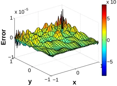
The solution computed by Chebyshev-PGD method for discretization of (100 × 100) with only 6 modes is shown in Fig.(2.8(a)). The error between the method proposed in this work with a 2D Finite difference method for the same discretization is given in Fig.(2.8(b)). We see that the method rapidly achieves a high level of accuracy.
The different PGD modes (enrichments in the solution) for this problem are also plotted in Fig.(2.9(a)). The L − 2error between PGD solution and the FD solution
vs the number of PGD modes is shown in Fig.(2.9(a)), where the L2Error in the
Fig.(2.9(b)) is used: Error = R Ω(UP GDn − Uref)2dΩ R ΩUref2 dΩ (2.62) we see that the PGD method for the Laplace problem is converged very fast.
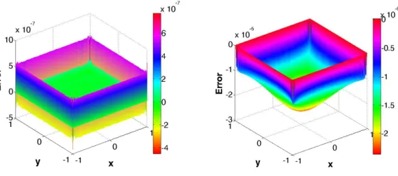
This problem have an analytical solution, when we compare the PGD solution and the Finite Difference solution with the analytical solution with the same grids number (100×100), we can see that the PGD method have a higher accuracy than the
Finite Difference method solution from the Figure(2.10). And the PGD convergence
2.3. Numerical results
(a) PGD solution (b) PGD Error with FD solution
Figure 2.8: Result for laplace problem
−1 −0.5 0 0.5 1 −0.5 0 0.5 y Y(y) −1 −0.5 0 0.5 1 −0.5 0 0.5 x X(x) (a) PGD modes 0 5 10 15 20 10−10 10−5 100 Modes number Error L−2 Error with FD (b) PGD convergence
Figure 2.9: PGD modes and PGD convergence
2.3.2 4th order PDE problem
Now, we consider the 2-D bi-harmonic problem in([Kirby and Yosibash, 2003]), which corresponds to a model for the deflection of a plate:
42u = f (x, y) in Ω = [−1, 1]2 (2.63)
where
f (x, y) = −8π4[cos(2π2x)sin2(πy) + sin2(πx)cos(2πy) − cos(2πx)cos(2πy)] (2.64)
u = 0 and ∂u
(a) PGD Error with Exact solution (b) FD Error with Exact solution
Figure 2.10: Error for PGD and FD solution compare with exact solution
0 5 10 15 20
10−10 100
Modes number
Error
L−2 Error with analytical solution
Figure 2.11: L − 2 Error for PGD and Exact solution VS PGD modes
This problem can be solved analytically and the exact solution for the deflection is given by:
u(x, y) = sin2(πx)sin2(πy) (2.66)
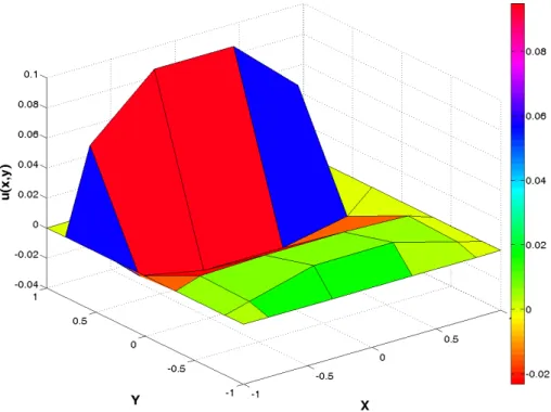
The exact solution and the solution by the PGD method for discretization of (100 × 100) are shown in Figure(2.12).
2.3. Numerical results
(a) Exact solution (b) PGD solution
Figure 2.12: Exact solution and PGD solution
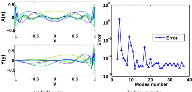
The PGD modes are shown in Figure(2.13(a)). The convergence of the method with the number of PGD modes is illustrated in Figure(2.13(b)).Where the L2 norm
Error (as Eq.(2.62)) is used for evaluate the PGD convergence; we can see that the
PGD solution converges very fast, as we can see from the exact solution, it is only one modes needed for the solution. And the error between the solution by PGD and
the exact solution is shown in Figure(2.14).
−1 −0.5 0 0.5 1 −0.5 0 0.5 y Y(y) −1 −0.5 0 0.5 1 −0.5 0 0.5 x X(x) (a) PGD mode 0 5 10 15 20 10−30 10−20 10−10 100