HAL Id: halshs-00406460
https://halshs.archives-ouvertes.fr/halshs-00406460
Submitted on 22 Jul 2009
HAL is a multi-disciplinary open access
archive for the deposit and dissemination of
sci-entific research documents, whether they are
pub-lished or not. The documents may come from
teaching and research institutions in France or
abroad, or from public or private research centers.
L’archive ouverte pluridisciplinaire HAL, est
destinée au dépôt et à la diffusion de documents
scientifiques de niveau recherche, publiés ou non,
émanant des établissements d’enseignement et de
recherche français ou étrangers, des laboratoires
publics ou privés.
Rudolf Berghammer, Agnieszka Rusinowska, Harrie de Swart
To cite this version:
Rudolf Berghammer, Agnieszka Rusinowska, Harrie de Swart. An Interdisciplinary Approach to
Coalition Formation. European Journal of Operational Research, Elsevier, 2009, pp. 487-496.
�halshs-00406460�
Formation
!Rudolf Berghammer1, Agnieszka Rusinowska2 and Harrie de Swart3 1 Institute of Computer Science, University of Kiel
Olshausenstraße 40, 24098 Kiel, Germany [email protected]
2 GATE, CNRS - Universit´e Lumi`ere Lyon 2
93, Chemin des Mouilles - B.P.167, 69131 Ecully Cedex, France [email protected]
3 Department of Philosophy, Tilburg University
P.O. Box 90153, 5000 LE Tilburg, The Netherlands [email protected]
Abstract. A stable government is by definition not dominated by any other government. However, it may happen that all governments are dominated. In graph-theoretic terms this means that the dominance graph does not possess a source. In this paper we are able to deal with this case by a clever combination of notions from different fields, such as relational algebra, graph theory and social choice theory, and by us-ing the computer support system RelView for computus-ing solutions and visualizing the results. Using relational algorithms, in such a case we break all cycles in each initial strongly connected component by remov-ing the vertices in an appropriate minimum feedback vertex set. In this way we can choose a government that is as close as possible to being un-dominated. To achieve unique solutions, we additionally apply the majority ranking recently introduced by Balinski and Laraki. The main parts of our procedure can be executed using the RelView tool. Its so-phisticated implementation of relations allows to deal with graph sizes that are sufficient for practical applications of coalition formation.
Corresponding author: Harrie de Swart, Tilburg University, Department of Philosophy, P.O. Box 90153, 5000 LE Tilburg, The Netherlands. e-mail: [email protected]
JEL Classification: D85, C63, C88, D71, D72
Keywords: Graph theory, RelView, relational algebra, dominance, stable gov-ernment
!Co-operation for this paper was supported by European COST Action 274 ‘Theory
1
Introduction
In Rusinowska et al. [15] a government is defined as a pair consisting of a coali-tion (a set of of parties) and a policy. Different governments may have different utilities (values) for the different parties. In Berghammer et al. [6] we have shown how the notion of ‘government g dominates government h’ can be described in terms of relational algebra. This enabled us to use the Kiel RelView tool for computing and visualizing the dominance relation. The governments that are un-dominated are by definition the stable ones.
Unfortunately, in practical applications stable government may not exist. In this paper we continue the work of Berghammer et al. [6] and deal with the problem what to do when there is no un-dominated government. Using graph-theoretic terms this means that the dominance graph does not possess a source. By a clever combination of well known concepts from different domains (re-lational algebra, the RelView tool for the manipulation and visualization of relations, graph theory, and the recently introduced majority ranking of [2]) we are able to deal with this case and to choose a government which is as close as possible to stable. As in Berghammer et al. [6], the decisive parts of our proce-dure are formulated as relational expressions and programs, respectively, so that RelView can be used for executing them and for visualizing the results.
The remainder of the paper is organized as follows. In Section 2 we present the model of coalition formation. Section 3 introduces some preliminaries from relational algebra, gives an overview on RelView, and recalls the method of Berghammer et al. [6] for computing the dominance relation with the help of this tool. Section 4 forms the core of the paper. We describe a general procedure for choosing a government in the case that there is no stable one. In the graph theoretical part we compute initial strongly connected components and minimum feedback vertex sets. If our procedure results in more than one government, we apply the recently introduced majority ranking of [2] to select one of them.
2
The Model of Coalition Formation
In this section, we briefly recall some of the main ideas of the model of coalition formation presented in Rusinowska et al. [15], i.e., the notions essential for the application of relational algebra and RelView to the model. Let N be the finite set of political parties and P be the finite set of all policies. A set of parties, i.e., an element of the powerset 2N, is called a coalition. We define a government as
a pair consisting of a coalition and a policy. Hence,
G :={ (S, p) | S ∈ 2N
∧ p ∈ P }
denotes the set of all governments. Usually, we assume that only a majority coalition (i.e., a coalition with more than half of the total number of seats in Parliament) can form a government. Nevertheless, one may easily imagine a government formed by a minority coalition.
Each party is assumed to have preferences on all policies and on all coalitions. Then a coalition is called feasible if it is acceptable to all its members. A policy is
feasible for a given coalition if it is acceptable to all members of that coalition and
a government is said to be feasible if it consists of a feasible coalition and a policy feasible for that coalition. By G∗ we denote the set of all feasible governments:
G∗:= { g ∈ G | G is feasible } .
For each i ∈ N, we assume a utility function U(i) : G → R, where U(i)(g)
denotes the utility (or value) of the government g ∈ G to party i ∈ N. A precise description of the utility of a government to a party has been given in Rusinowska et al. [15]. In Roubens et al. [13], the MacBeth technique has been applied to determine these utilities.
A feasible government g = (S, p) ∈ G∗ dominates a feasible government h∈ G∗ (denoted as g $ h) if the property
(∀ i ∈ S : U(i)(g) ≥ U(i)(h)) ∧ (∃ i ∈ S : U(i)(g) > U(i)(h))
holds. We call “$” the dominance relation and the directed graph (G∗,$) the dominance graph. A feasible government is said to be stable if it is dominated
by no feasible government. By
SG∗:= {g ∈ G∗| ¬ ∃ h ∈ G∗: h $ g}
we denote the set of all (feasible) stable governments. Using graph-theoretic terminology, SG∗ is the set of all sources (or initial vertices) of the dominance
graph.
In Rusinowska et al. [15] necessary and sufficient conditions for the existence and the uniqueness of stable governments are investigated and, in addition, some variants of the notion of stability are discussed. All this shows that the above definition seems to be the most natural one. Therefore, we also use it in the present paper.
3
Computing the Dominance Relation with RelView
In this section, we first present the basics of relational algebra and indicate how sets can be modeled. For more details, see e.g., Schmidt and Str¨ohlein [16] or Brink et al. [12]. After a short introduction to the RelView tool, we then recall how the dominance relation can be computed and visualized with this tool. 3.1 Relational Algebra and RelViewIf X and Y are sets, then a subset R of the Cartesian product X × Y is called a (binary) relation with domain X and range Y . We denote the set (in this context also called type) of all relations with domain X and range Y (i.e., the powerset of X × Y ) by [X ↔ Y ] and write R : X ↔ Y instead of R ∈ [X ↔ Y ]. If X and
Y are finite sets of size m and n respectively, then we may consider a relation R : X↔ Y as a Boolean matrix with m rows and n columns. The Boolean
matrix interpretation of relations is well suited for many purposes and also used as one of the graphical representations of relations within the RelView tool. Therefore, in this paper we often use Boolean matrix terminology and notation. In particular, we write Rx,y instead of *x, y+ ∈ R or x R y.
In the present paper we will use the following basic operations on relations:
R (complement), R ∪ S (union), R ∩ S (intersection), RT(transposition) and
R; S (composition). Complement, union, and intersection are the set-theoretic
operations on the complete Boolean lattices [X ↔ Y ]. Hence, for all x ∈ X and
y∈ Y we have Rx,y if and only if ¬Rx,y, (R ∪ S)x,y if and only if Rx,y or Sx,y,
and (R ∩ S)x,y if and only if Rx,y and Sx,y. The transposition RT of a relation R : X↔ Y has type [Y ↔ X] and is defined by the equivalence of Rx,y and Ry,xT
for all x ∈ X and y ∈ Y . A composition R; S is only defined if the range of R coincides with the domain of S. In the case R : X ↔ Y and S : Y ↔ Z we have the typing R; S : X ↔ Z and for all x ∈ X and z ∈ Z that (R; S)x,z if and only
if there exists y ∈ Y such that Rx,y and Sy,z.
Besides the above basic operations we will use the special relations O (empty
relation), L (universal relation), and I (identity relation), one for each type. Here
we overload the symbols. This means that we avoid the binding of the types to the symbols for these special relations via subscripts (as in OXY) or superscripts
(as in OXY). This is due to the fact that the types can be re-constructed from the
context. The first two constants O and L are the smallest and greatest element of the complete Boolean lattices [X ↔ Y ], respectively, the third one I is the relation-level equivalent of set-theoretic equality. The latter means that each of the equal designated relations I has a type of the form [X ↔ X] and is defined by the equivalence of Ix,y and x = y, for all x, y ∈ X.
If R : X ↔ Y is included in S : X ↔ Y we write R ⊆ S and equality of R and S is denoted as R = S. Hence, R ⊆ S if and only if for all x ∈ X and y ∈ Y from Rx,y it follows that Sx,y and R = S if and only if for all x ∈ X and y ∈ Y
both properties even are equivalent.
By R∗ we denote the reflexive-transitive closure of a relation R : X ↔ X.
This closure is introduced via the equation R∗ = !
i≥0Ri, where the powers Ri of R are inductively defined by R0 = I and Ri+1 = R; Ri. Applying
graph-theoretic terminology we obtain that R∗
x,y if and only if there is a path from the
vertex x to the vertex y in the directed graph (X, R).
Relational algebra offers some simple and elegant ways to describe subsets of a given set or, equivalently, predicates on this set. In this paper we will use vectors, membership-relations, and injective embeddings for this task.
A vector v is a relation v with v = v; L. In the Boolean matrix model this condition means that each row either consists of ‘true’ entries only or consists of ‘false’ entries only. As for a vector, therefore, the range is irrelevant, we consider in the following mostly vectors v : X ↔ 1 with a specific singleton set 1 := {⊥} as range and omit in such cases the second subscript, i.e., write vxinstead of vx,⊥.
vector v : X ↔ 1 can be considered as a Boolean matrix with exactly one column, i.e., as a Boolean column vector, and describes (or is a description of) the subset
{x ∈ X | vx} of X. If a vector describes a singleton set, i.e., an element of its
domain, it is called a point.
As a second way to model sets we will use the relation-level equivalents of the set-theoretic symbol “∈”, i.e., membership-relations M : X ↔ 2X. These specific
relations are defined by Mx,Y if and only if x ∈ Y , for all x ∈ X and Y ∈ 2X.
A Boolean matrix representation of M requires exponential space. However, in Berghammer et al. [4] an implementation of M using ordered binary decision diagrams is presented, the number of vertices of which is linear in the size of X. If the vector v describes a subset Y of X, then inj (v) : Y ↔ X denotes the
injective embedding of Y into X. This means that for all y ∈ Y and x ∈ X we
have inj (v)y,x if and only if y = x. A combination of injective embeddings and
membership-relations allows a column-wise enumeration of sets of subsets. More specifically, if v describes a subset S of 2X in the sense defined above, then for
all x ∈ X and Y ∈ S we have (M; inj (v)T)
x,Y if and only if x ∈ Y . Using matrix
terminology this means that the elements of S are described precisely by the columns of the relation M; inj (v)Tof type [Y ↔ X].
Relational algebra has a fixed and surprisingly small set of constants and operations which (in the case of finite carrier sets) can be implemented very efficiently. At Kiel University we have developed a computer system for the visualization and manipulation of relations and for relational prototyping and programming, called RelView. The tool is written in the C programming lan-guage, uses ordered binary decision diagrams for implementing relations, and makes full use of the X-windows graphical user interface. Details and applica-tions can be found, for instance, in Berghammer et al. [5], Behnke et al. [3], Berghammer et al. [4], and Berghammer et al. [7].
The main purpose of RelView is the evaluation of relation-algebraic ex-pressions. These are constructed from the relations of its workspace using pre-defined operations and tests, user-pre-defined relational functions, and user-pre-defined relational programs. A relational program is much like a function procedure in the programming languages Pascal or Modula 2, except that it only uses relations as data type. It starts with a head line containing the program name and the for-mal parameters. Then the declaration of the local relational domains, functions, and variables follows. Domain declarations can be used to introduce projection relations and pairings of relations in the case of Cartesian products, and injec-tion relainjec-tions and sums of relainjec-tions in the case of disjoint unions, respectively. The third part of a program is the body, a while-program over relations. As a program computes a value, finally, its last part consists of a return-clause, which is a relation-algebraic expression whose value after the execution of the body is the result.
3.2 Computing and Visualizing Dominance
In Berghammer et al. [6] we have developed a relation-algebraic specification of dominance and stability. To this end, we supposed a relational description of
government membership and the parties’ utilities to be given. The first means that we have a relation M : N ↔ G∗at hand such that for all i ∈ N and g ∈ G∗
Mi,g ⇐⇒ party i is a member of government g;
the second means that we have for each party i ∈ N a relation R(i) : G∗↔ G∗
at hand such that for all g, h ∈ G∗.
R(i)g,h ⇐⇒ U(i)(g) ≥ U(i)(h) .
Based on the relations R(i), i ∈ N, we first introduced a global utility (or
comparison) relation C : N ↔ G∗×G∗by demanding for all i ∈ N and g, h ∈ G∗ Ci,$g,h% ⇐⇒ R(i)g,h
and transformed this component-based specification into a relation-algebraic (i.e., component-free) one. Then we proved the following fact: If π : G∗×G∗↔ G∗
and ρ : G∗×G∗↔ G∗are the projection relations of the direct product G∗× G∗
and the vector DomVec(M, C) : G∗×G∗↔ 1 is defined by
DomVec(M, C) = (π; MT∩ CT); L ∩ (π; MT∩ E; CT); L , (1)
where E := ρ; πT∩ π; ρT: G∗×G∗↔ G∗×G∗is the so-called exchange relation1,
then we have for all *g, h+ ∈ G∗×G∗that DomVec(M, C)
$g,h%if and only if g $ h.
Hence, equation (1) is a relation-algebraic specification of the dominance relation with the government membership relation M and the global utility relation C as its input.
Strictly speaking, according to (1) dominance is specified as a vector of type [G∗×G∗↔ 1]. But what we really wanted is a specification as a relation
of type [G∗↔ G∗]. So, we additionally had to apply the technique of Schmidt
and Str¨ohlein [16] for transforming a vector with a direct product as domain into the corresponding relation. Doing so, we obtained a relation-algebraic spec-ification DomRel(M, C) : G∗↔ G∗ of the dominance relation by
DomRel(M, C) = πT; (ρ ∩ DomVec(M, C); L) . (2)
Both equations (1) and (2) can be used for specifying relation-algebraically the vector description StabVec(M, C) : G∗↔ 1 of the set SG∗ of all stable
gov-ernments. We used (1) and arrived after some steps at
StabVec(M, C) = ρT; DomVec(M, C) . (3)
We immediately could transform the three relation-algebraic specifications (1), (2), and (3) into the programming language of RelView. In the first case
1 This name stems from the fact that for all u, v
∈ G∗× G∗we have Eu,v if and only
the result is the following program: DomVec(M,C)
DECL Prod = PROD(M^*M,M^*M); pi, rho, E
BEG pi = p-1(Prod); rho = p-2(Prod); E = rho*pi^ & pi*rho^
RETURN -dom(pi*M^ & -C^) & dom(pi*M^ & E*-C^) END.
Here the first declaration introduces Prod as a name for the direct product
G∗× G∗. Using Prod, the projection relations and the exchange relation are
then computed by the three assignments of the body and stored as pi, rho, and E, respectively. The return-clause of the program consists of a direct trans-lation of (1) into RelView-syntax, where ^, -, &, and * denote transposition, complement, intersection, and composition, and, furthermore, the operation dom computes for a relation R : X ↔ Y the vector R; L : X ↔ 1.
Similarly, by straightforward translations we obtained RelView-implemen-tations of the remaining two relation-algebraic specifications.
Here is the RelView-code for specification (2): DomRel(M,C)
DECL Prod = PROD(M^*M,M^*M); pi, rho
BEG pi = p-1(Prod); rho = p-2(Prod)
RETURN pi^ * (rho & DomVec(M,C) * L1n(C)) END.
A translation of specification (3) into the programming language of the tool, finally, led to the following relational program:
StabVec(M,C)
DECL Prod = PROD(M^*M,M^*M); rho
BEG rho = p-2(Prod)
RETURN -(rho^ * DomVec(M,C)) END.
The operation L1n of the RelView-program DomRel computes for a relation R :
X↔ Y the universal relation L of the specific type [1 ↔ Y ], in matrix terminology
hence a Boolean universal row vector.
4
The Case of no Stable Government
Having computed the dominance relation, three cases may occur: there are mul-tiple stable governments, there is exactly one stable government, and a stable government may not exist.
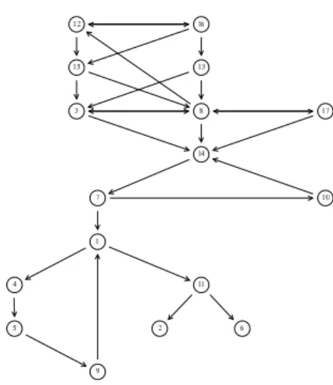
Fig. 1. Dominance without a stable government
Based on the situation in Poland after the 2001 elections, in Berghammer et al. [6] we obtained an example for the first case, viz. a dominance graph with three sources, representing the three different stable governments. In such a situation one might allow negotiations in order to choose a government from among the stable ones; see Rusinowska and de Swart [14]. An alternative is to select a specific stable government that may be considered as more attractive than the other stable ones via the majority ranking, recently introduced by Balinski and Laraki [2], see Sections 4.5 and 4.6.
If there is exactly one stable government (i.e., one source), then obviously this one has to be selected.
In the remainder of this section we continue the work of Berghammer et al. [6] and concentrate on the third case of no stable government. This means that the dominance graph has no source, like in the RelView-picture of Fig. 1. The situation described by this graph appears if we change the utilities of the example of Berghammer et al. [6] a little bit. As in the original case, for reasons of clearness the picture shows a transitive reduction of the dominance graph only, i.e., a minimal subgraph such that the reflexive-transitive closures of the subgraph and of the original graph coincide.
Assuming that a computed dominance graph has no source, in Section 4.1 we first describe our procedure to select a government as close as possible to being stable. After that we go into details and show how to compute initial strongly connected components (Section 4.2) and minimum feedback vertex sets relation-algebraically (Section 4.3). In Section 4.4 we demonstrate the application of our procedure to Fig. 1. If our procedure yields several governments that are as close as possible to being stable, as is the case in our example, we use the majority ranking of [2] to select the ‘most preferred’ one of them. In Section 4.5 we apply the majority ranking of Balinski and Laraki to our example. This will help to
understand in Section 4.6 the general description of the majority ranking and some of its nice properties.
4.1 The General Approach
If the computed dominance graph has no source, i.e., there exists no stable gov-ernment, the central question is which government should be chosen. In this section we answer this question by proposing a procedure for choosing a govern-ment that can be considered as close as possible to being stable.
As a whole, our proposal is presented below. In it, we apply some well-known concepts from graph theory. First, we use strongly connected components (SCCs), i.e., maximal sets of vertices such that each pair of vertices is mutually reachable. Especially we are interested in SCCs without arcs leading from outside into them. These SCCs are said to be initial. We also use minimum feedback vertex sets, where a feedback vertex set (FVS) is a set of vertices that contains at least one vertex from every cycle of the graph. And here is our procedure:
1. Compute the set I of all initial SCCs of the dominance graph. 2. For each SCC C from I do:
a) Compute the set F of all minimum FVSs of the subgraph gener-ated by the vertices of C.
b) Select from all sets of F with a maximal number of ingoing arcs one with a minimal number of outgoing arcs. We denote this one by F .
c) Break all cycles of C by removing the vertices of F from the dominance graph.
d) Select an un-dominated government from the remaining graph. If there is more than one candidate, use the majority ranking of [2] to select the ‘most preferred’ one.
3. If there is more than one set in I, select the final stable government from the results of the second step by applying the majority ranking of [2] again.
An outgoing arc of the dominance graph denotes that the government in ques-tion dominates another one and an ingoing arc denotes that the government in question is dominated by another one. Hence the governments of an initial SCC can be seen as a cluster which is not dominated from outside.
For each initial strongly connected component, we compute in step 2 the set of all minimum feedback vertex sets, where a minimum feedback vertex set is a minimal set of vertices which breaks all cycles. Next, we choose a specific minimum feedback vertex set according to the following rule. First, we choose the set(s) for which the number of ingoing arcs is maximal. Since an ingoing arc denotes that a government is dominated, such a choice means selecting gov-ernments dominated most frequently. Next, if there are at least two such sets, we choose one for which the number of outgoing arcs is minimal, meaning the choice of the governments which dominate other governments least frequently.
Next, we break all cycles by removing the chosen set of governments. This cor-responds to a removal of those candidates which are ‘least attractive’ for two reasons: because they are most frequently dominated and they dominate other governments least frequently. In Section 4.4 we will apply this approach to the example given in Fig. 1.
At this place it should be mentioned that the application of steps 1 and 2 may not lead to a unique solution. In this case we proceed as in the case of multiple stable governments to select the final government from among the ‘graph-theoretical’ results, see Sections 4.5 and 4.6.
4.2 Computing Initial Strongly Connected Components
Given a finite graph (V, R) with relation R : V ↔ V for the arcs, the SCCs of (V, R) are precisely the equivalence classes of the equivalence relation R∗∩(RT)∗.
The following RelView-program Classes for column-wisely enumerating the equivalence classes of an equivalence relation S : X ↔ X has been published in Berghammer and Fronk [8]. In it, the calls Ln1(S) and On1(S) compute the universal vector L : X ↔ 1 and the empty vector O : X ↔ 1, respectively, the call point(v)yields one of the points contained in the non-empty vector v, and the operation + computes the relational sum. In matrix terminology the latter means that it puts the matrices one upon the other, so that the RelView-expression (C^ + c^)^of Classes ‘concatenates’ the matrix C and the vector c.
Classes(S) DECL C, v, c BEG C = On1(S); v = Ln1(S); WHILE -empty(v) DO c = S * point(v); IF isempty(C) THEN C = c ELSE C = (C^ + c^)^ FI; v = v & -c OD RETURN C END
Using the operation rtc for computing reflexive-transitive closures, from the above remark we obtain that the call Classes(rtc(R) & rtc(R^)) column-wisely enumerates the SCCs of R.
In Berghammer and Fronk [8] the authors also refine the program Classes to a RelView-program that computes the initial SCCs of R. Essentially this refinement consists of an additional assignment in front of the hitherto first assignment to compute rtc(R) & rtc(R^) and to store the result as S (which now is a local variable instead of the formal parameter), and it simply checks after the computation of the next equivalence class c via the assignment c = S * point(v) whether c is initial and executing only in that case the conditional of the original
while-loop. It leads to the following program: InitSccs(R) DECL S, C, v, c BEG S = rtc(R) & rtc(R^); C = On1(S); v = Ln1(S); WHILE -empty(v) DO c = S * point(v); IF incl(R*c,c) THEN IF isempty(C) THEN C = c ELSE C = (C^ + c^)^ FI FI; v = v & -c OD RETURN C END
The RelView-expression incl(R*c,c) of InitSccs tests whether the vector R*c(describing the predecessors of c with respect to R) is contained in c which, in words, exactly means that the SCC described by c is initial.
4.3 Computing Minimum Feedback Vertex Sets
The following relation-algebraic computation of minimum FVSs follows the lines of Berghammer and Fronk [9]. As in Section 4.2 we assume that (V, R) is a finite graph with relation R : V ↔ V .
Let M : V ↔ 2V be the membership-relation on vertices. In a first step we
reduce the computation of the FVSs to the computation of simple cordless cycles, i.e., simple cycles c which do not contain a pair x, y of vertices that forms an arc in (V, R) but not an arc in c. Since a set F of vertices is a FVS if and only if it contains a vertex from every simple chordless cycle (Berghammer and Fronk [9]), it suffices to enumerate column-wisely the vertex sets of the simple chordless cycles of (X, R) via a relation K : V ↔ C, where C denotes the set of vertex sets of the simple chordless cycles. Assuming K to be at hand, for all F ∈ 2V we are
able to calculate as follows (where c ranges over the simple chordless cycles and
S ranges over C): F is a FVS ⇐⇒ ∀ c : ∃ x : x ∈ F ∧ x vertex of c ⇐⇒ ∀ S : ∃ x : Mx,F∧ Kx,S ⇐⇒ ¬∃ S : MT; K F S∧ LS ⇐⇒ MT; K; L F
This calculation yields MT; K; L : 2V
↔ 1 as the vector representation of all FVSs
of (V, R). Next we apply that the vector v∩Q; v describes the least elements of the set described by the vector v with respect to the preorder Q; see e.g., Schmidt and Str¨ohlein [16]. If we use the above vector as v, the size comparison relation on 2V
following program for computing the vector description of the minimum FVSs from the relation K:
MfvsVec(K)
DECL LeEl(Q,v) = v & -(-Q * v)); DECL M
BEG M = epsi(O(K))
RETURN LeEl(cardrel(O(K)),-dom(-(M^*K))) END.
From this program we obtain a program for the column-wise enumeration of the minimum FVSs by applying the technique described in Section 3.1.
We call a set S of vertices of (V, R) progressively infinite if it is non-empty and for each vertex x ∈ S there exists a successor y ∈ S. Fundamental for obtaining a relation-algebraic specification of the relation K : V ↔ C (a task we still have to solve) is the following fact (Berghammer and Fronk [9]): S is the vertex set of a simple chordless cycle if and only if it is a minimal progressively infinite set. Thus, our next goal is identified. We have to develop a RelView-program, say MprinfVec, that computes the vector description of the minimal progressively infinite sets. Then the technique of Section 3.1 shows that K is computed by
M * inj(MprinfVec(R))^ .
In order to obtain a vector that describes the minimal progressively infinite sets, we first neglect minimality and calculate for a set S of vertices as follows:
S progr. infinite ⇐⇒ (∃ x : x ∈ S) ∧ (∀ x : x ∈ S → ∃ y : y ∈ S ∧ Rx,y) ⇐⇒ (∃ x : Mx,S) ∧ (∀ x : Mx,S → ∃ y : My,S∧ Rx,y) ⇐⇒ (∃ x : L⊥,x∧ Mx,S) ∧ (∀ x : Mx,S → (R; M)x,S) ⇐⇒ (L; M)⊥,S∧ (¬∃ x : L⊥,x∧ Mx,S∧ R; Mx,S ⇐⇒ (L; M)TS∧ L; (M ∩ R; M)⊥,S ⇐⇒ ((L; M)T∩ L; (M ∩ R; M)T)S Hence, (L; M)T ∩ L; (M ∩ R; M)T: 2V
↔ 1 is a vector description of the
progres-sively infinite sets of the graph (V, R). Minimalization now is obtained by using two well known results: MT; M : 2V
↔ 2V relation-algebraically specifies set
in-clusion on 2V and the vector v ∩(QT∩ I)v describes the minimal elements of the
set described by the vector v with respect to the preorder Q; see again Schmidt and Str¨ohlein [16]. If we combine these facts with the vector description of the progressively infinite sets and formulate the result in RelView-syntax, we arrive
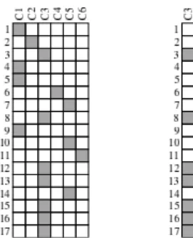
Fig. 2. SCCs and initial SCC of the former example
at the following RelView-program: MprinfVec(R)
DECL Min(Q,v) = v & -((Q^ & -I(Q)) * v); M, SI, L
BEG M = epsi(O(R)); SI = -(M^ * -M); L = L1n(R)
RETURN Min(SI, (L*M)^ & -(L * (M & -(R*M)))^) END.
The bottleneck of this program is the use of set inclusion since the size of the ordered binary decision diagrams of this relation is exponential in the size of the base set. Using the present RelView-version it can be only applied to graphs with up to approximately 30 vertices. As we apply it, however, only to initial SCCs, this usually suffices for practical applications of coalition formation. It still should be mentioned that Berghammer and Fronk in [8] develop a refinement of our programs that avoids the use of set inclusion and can be used for graphs consisting of about 100 vertices in general and even more in advantageous cases. 4.4 The Example Revisited
In the following, we want to demonstrate an application of the RelView-programs we have developed so far. As input we assume the dominance relation, the transitive reduction of which graphically is depicted in Fig. 1.
Following the general procedure of Section 4.1, in the first step we have to compute the initial SCCs using the RelView-program InitSccs of Section 4.2. The graph of Fig. 1 possesses exactly one initial SCC. Its RelView-represen-tation as Boolean vector is shown on the right-hand side of Fig. 2. To give an impression how a column-wise enumeration of sets of subsets looks in RelView, on the left-hand side of the figure we additionally show the six SCCs of the input as 17 × 6 matrix. In both cases labels are added to rows and columns by a specific feature of the tool for illustration purposes. In RelView a black square of a Boolean matrix means ‘true’ and a white square means ‘false’. Hence, the
Fig. 3. Minimum FVSs of the initial SCC
SCCs of the input are {1, 4, 5, 9}, {2}, {3, 8, 12, 13, 15, 16, 17}, {6}, {7, 10, 14}, and {11}. The only initial SCC is C3= {3, 8, 12, 13, 15, 16, 17}.
Next, we perform Step a) of the general procedure to the initial SCC. C3
contains the cycles {12, 16}, {3, 8}, {8, 12, 15}, {3, 8, 12, 15}, {8, 12, 16, 13},
{8, 12, 16, 15} and {3, 8, 12, 16, 15}. By means of the RelView-program
MfvsVecof Section 4.3 we obtain two minimum FVSs, viz. {8, 16} and {8, 12}. The Boolean RelView-matrix of Fig. 3 column-wisely enumerates these sets.
Since Step a) of the general procedure of Section 4.1 demands to compute the minimum FVSs of the subgraph generated by the initial SCC C3, strictly
speaking we first get a relation of type [C3↔ F] as result, which means that the
elements of F are considered as subsets of C3. The matrix of Fig. 3 is obtained
from this result by multiplying it from the left with inj (v)T, where the vector
v : G∗↔ 1 describes the SCC C3. Thus, the computed minimum FVSs become
subsets of the set G∗.
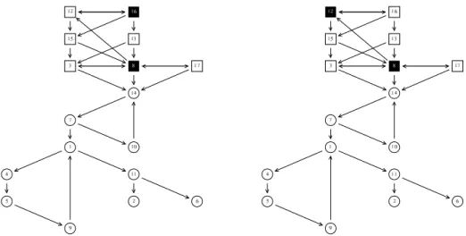
That {8, 16} and {8, 12} are indeed the only minimum FVS hopefully be-comes clear if we consider Fig. 4. It shows two copies of the input graph of Fig. 1. In both cases we have instructed RelView to draw the vertices of the initial SCC as squares and additionally to indicate a minimum FVS by the colour black. In the graph on the left-hand side we identify the minimum FVS {8, 16} and in the other graph the minimum FVS {8, 12}. From Fig. 4 we also see that five arcs lead from outside into the FVS {8, 12}, but only four arcs lead from outside into {8, 16}. Hence, by Steps b) and c) of the general procedure we have to remove the vertices 8 and 12 from the graph, which leads to 16 and 17 as new sources, i.e., as governments that can be considered as being as close as possible to stable. What government finally is chosen is determined by applying the majority ranking, recently introduced by Balinski and Laraki in [2]. 4.5 Application of the Majority Ranking
According to the procedure described in Section 4.1, if the application of graph theory does not give a unique solution, we select the final government from among the ‘graph-theoretical’ results by applying the majority ranking, recently introduced by M. Balinski and R. Laraki [2].
They blame Arrow’s impossibility results on the fact that the social choice or welfare functions take individual orderings of the alternatives as input. But in general the individual agents do not speak the same language: when agent 1 says that he prefers A to B he may mean something quite different than when agent 2 says the same thing; agent 1 may mean that A is slightly better than B, while agent 2 may mean that A is fine but B is repulsive. So, Balinski and Laraki argue that it is no surprise that different election mechanisms yield different outcomes and that there is no social choice or welfare function that satifies all of some well-known properties. By looking at contests in real life, they realized that the agents should speak the same language by sharing a common grading system, for instance the rankings {A, B, C, D, E} in the American school system. And they proved that in this new framework a unique social grading function exists that has very nice properties.
Note that by giving grades to the alternatives in some common grading sys-tem much more information is provided by the voters/judges than in the case of giving rankings of the alternatives.
First, we will demonstrate Balinski and Laraki’s procedure in our example above and next we will describe their procedure in more general terms.
In the example of Section 4.4 there was no undominated government. By ap-plying ‘graph-theoretical’ techniques we found two governments g16= (AC, p16)
and g17= (AB, p17) that are as stable as possible in the sense specified in
Sec-tion 4.1; here {A, C} is the coaliSec-tion of g16 and p16 denotes the policy of g16;
similarly for AB and p17 in g17. The dominance graph in our example shows
which governments dominate other governments, where domination is defined in terms of the utilities UI(g) of the different governments g for the different
[13]), on a fixed grading scale, say from 0 till 100. Let us assume that for party
A we have the utilities
UA(g16) = 60, UA(g17) = 70,
for party B we have the utilities
UB(g
16) = 45, UB(g17) = 40
(which means that B dislikes A a lot) and for party C we have the utilities
UC(g16) = 50, UC(g17) = 0
(saying that C finds B repulsive). So, we have two alternatives g16 and g17 and
three judges/parties A, B and C. Balinski and Laraki’s matrix of judgements, or profile, consequently looks as follows:
A B C g16 g17 "60 45 50 70 40 0 #
Applying Balinski and Laraki’s majority-grade fmaj to each row (alternative)
we find:
fmaj(60, 45, 50) = 50 and fmaj(70, 40, 0) = 40.
This gives rise to the following majority ranking: g16 $maj g17. So, in our
ex-ample g16 is the most preferred, as stable as possible, government to be chosen
from the seventeen available non-stable governments. 4.6 General Description of the Majority Ranking
As in the traditional framework of Arrow, there is a finite set C of m competitors, governments in our case, a1, . . . , am, and a finite set J of n judges, in our case
parties, 1, . . . , n. Furthermore, a common language L is required, in our case the fixed set of possible utilities {0, 1, . . ., 100}. L is a set of strictly ordered grades
rn, and may be finite or an interval of the real numbers. We take ri 2 rj to
mean that riis a higher grade than rj or ri= rj. The input for a social grading
function (SGF) is then a m by n matrix, called a profile, filled with grades (i.e., elements of L), meaning that every competitor (m rows) is given a grade by every judge (n columns). A method of grading is a function F that assigns to every profile one output, called the final grade, which is an m-tuple of grades (one grade for each competitor, following the order of competitors used in the input matrix).
A function f from n-tuples (the grades given to a competitor by the n judges) to a single grade, the final grade of the competitor, is called an aggregation
function if and only if it satisfies the conditions of Anonymity, Unanimity and
Balinski and Laraki formulate the following six properties for a Social Grad-ing Function: Neutrality, Anonymity, Unanimity, Monotonicity, IIA and Conti-nuity (see [2]) and prove the following Theorem.
Theorem A method of grading F satisfies the six properties just mentioned if and only if there exists an aggregation function f such that the output of F is given by applying f to all the competitors in the input matrix (profile) of F . So, we have the following picture:
1 . . . n r11 . . . r1n ... ... ... rm1. . . rmn →F (f(r11, . . . , r1n), . . . , f(rm1, . . . , rmn))
We call F an SGF if and only if F satisfies the six properties given above. The question is if there is a single best aggregation function f, and thus a single best SGF F . Balinski and Laraki consider order functions: the kth order function
fk takes as input an n-tuple of grades and gives as output the kth highest grade.
Balinski and Laraki conclude that these order functions are demonstrably best for aggregating. In particular they are very good at avoiding or minimizing manipulability ([2]).
There are many order-functions. But one in particular is clearly superior to all its competitors, namely the middlemost aggregation function f. Suppose r1 ≥
r2≥ . . . ≥ rn. A middlemost aggregation function f is defined by: f (r1, . . . , rn) = r(n+1)/2
when n is odd, and
rn/2≥ f(r1, . . . , rn) ≥ r(n+2)/2
when n is even. So, when n is odd the order function f(n+1)/2 is the middlemost
aggregation function. When n is even, there are infinitely many. In particular
fn/2 is the upper-middlemost and f(n+2)/2 the lower-middlemost aggregation
function. Any grade not bounded by the middlemost aggregation functions is condemned by an absolute majority of judges as either too high or too low. And the middlemost aggregation functions have nice properties, see [2].
The majority-grade fmaj is defined by:
f(n+1)/2when n is odd, and
f(n+2)/2when n is even.
We now have a method to grade. The new model now allows us to use this grading method to construct a ranking method (the traditional framework of Arrow did not offer this option).
ai$majaj:= fmaj(ai) > fmaj(aj)
If fmaj(a
i) = fmaj(aj), then the majority-grade is dropped from the grades of
both competitors and the procedure is repeated for these alternatives.
Balinski and Laraki prove that the majority-ranking has a number of nice properties, among which the following.
Theorem The majority-ranking always ranks one competitor ahead of another unless the judges have assigned the two competitors identical grades.
In obtaining these results, it is crucial that there is a common language for the judges to use. When there is no common language, the only meaningful input a judge can give is the order of his preferences, which is a serious loss of information and in fact brings us back to the old framework of social choice theory. In this case, the impossibility theorems of social choice theory [1] also resurface.
5
Conclusions
The central concepts of the coalition formation model are the notion of (feasible) government and the notion of stable government. The latter is defined as a feasible government dominated by no feasible government. In the present paper, we aim to answer the question which government should be chosen if there is no stable government (that is, if the dominance graph has no source).
The attractiveness and novelty of our approach consists in: 1. the clever combination of notions from partly different domains (relational algebra, graph theory and very recent methods from social choice theory), and 2. the immediate and easy support by the computer system RelView for computing solutions and for visualizing the results.
Starting from a situation in which there is no stable government, the pro-cedure given in Section 4.1 breaks all cycles in each initial strongly connected component by removing the vertices in an appropriate minimum feedback vertex set; this corresponds to a removal of those candidates which are ‘least attractive’ for two reasons: because they are most frequently dominated and they dominate other governments least frequently. In this way our procedure selects one or more governments that are as close as possible to being stable.
In case that our procedure yields more than one possible outcome, we select the final government (from the results of the procedure described above) by applying the majority ranking, recently introduced by Balinski and Laraki [2]. In this way we select, in case there is no stable government, a unique, most preferred, government which is as close as possible to being stable.
Of course, the majority ranking may also be used in case there is more than one stable government in order to select the most preferred of them.
Acknowledgement: We want to thank the unknown referees for their valuable remarks.
References
1. Arrow K.J., 1978. Social Choice and Individual Values. Yale University Press, 9th edition.
2. Balinski M. and Laraki R., 2006. A Theory of Measuring, Electing and
Rank-ing. Ecole Polytechnique, Cahier no 2006-11. Laboratoire d’Econometrie, Paris.
http://ceco.polytechnique.fr/
3. Behnke, R., Berghammer, R., Meyer, E., Schneider, P., 1998. RelView – A sys-tem for calculation with relations and relational programming. In: Astesiano, E., (Ed.), Proc. Conf. “Fundamental Approaches to Software Engineering (FASE ’98)”, LNCS 1382, Springer, pp. 318-321.
4. Berghammer, R., Leoniuk, B., Milanese, U., 2002. Implementation of relational algebra using binary decision diagrams. In: de Swart, H., (Ed.), Proc. 6th Int. Workshop “Relational Methods in Computer Science”. LNCS 2561, Springer, pp. 241-257.
5. Berghammer, R., von Karger, B., Ulke, C., 1996. Relation-algebraic analysis of Petri nets with RelView. In: Margaria, T., Steffen, B., (Eds.), Proc. 2nd Workshop “Tools and Applications for the Construction and Analysis of Systems (TACAS ’96)”. LNCS 1055, Springer, pp. 49-69.
6. Berghammer, R., Rusinowska, A., de Swart, H., 2007. Applying relational algebra and RelView to coalition formation. European Journal of Operational Research 178, 530-542.
7. Berghammer, R., Schmidt, G., Winter, M., 2003. RelView and Rath – Two systems for dealing with relations. In: de Swart, H., Orlowska, E., Schmidt, G., Roubens, M., (Eds.), Theory and Applications of Relational Structures as Knowl-edge Instruments. LNCS 2929, Springer, pp. 1-16.
8. Berghammer, R., Fronk, A., 2004. Considering design tasks in OO-software engi-neering using relations and relation-based tools. Journal on Relational Methods in Computer Science 1, 73-92.
9. Berghammer, R., Fronk, A., 2005. Exact computation of minimum feedback vertex sets with relational algebra. Submitted for publication.
10. Brams, S.J., Fishburn, P.C., 1983. Approval Voting. Birkh¨auser, Boston.
11. Brams, S.J., Fishburn, P.C., 2002. Voting Procedures. In: Arrow, K., Sen, A., Suzumura, K., (Eds.), Handbook of Social Choice and Welfare. Elsevier Science, Amsterdam.
12. Brink, C., Kahl, W., Schmidt, G., (Eds.), 1997. Relational Methods in Computer Science. Advances in Computing Science, Springer.
13. Roubens, M., Rusinowska, A., de Swart, H., 2006. Using MacBeth to determine utilities of governments to parties in coalition formation. European Journal of Operational Research 172/2, 588-603.
14. Rusinowska, A., de Swart, H., 2004. Negotiating a stable government - an applica-tion of bargaining theory to a coaliapplica-tion formaapplica-tion model. Submitted for publicaapplica-tion. 15. Rusinowska, A., de Swart, H., van der Rijt, J.W., 2005. A new model of coalition
formation. Social Choice and Welfare 24, 129-154.
16. Schmidt, G., Str¨ohlein, T., 1993. Relations and Graphs. Discrete Mathematics for Computer Scientists, EATCS Monographs on Theoret. Comput. Sci., Springer. 17. de Swart, H., van Deemen, A., van der Hout, E., Kop, P., 2003. Categoric and
ordinal voting: an overview. In: de Swart, H., Orlowska, E., Schmidt, G., Roubens, M., (Eds.), Theory and Applications of Relational Structures as Knowledge Instru-ments. LNCS 2929, Springer, pp. 147-196.