HAL Id: hal-02347891
https://hal.archives-ouvertes.fr/hal-02347891
Submitted on 5 Nov 2019
HAL is a multi-disciplinary open access
archive for the deposit and dissemination of
sci-entific research documents, whether they are
pub-lished or not. The documents may come from
teaching and research institutions in France or
abroad, or from public or private research centers.
L’archive ouverte pluridisciplinaire HAL, est
destinée au dépôt et à la diffusion de documents
scientifiques de niveau recherche, publiés ou non,
émanant des établissements d’enseignement et de
recherche français ou étrangers, des laboratoires
publics ou privés.
ASSESSING CROSS-DEPENDENCIES USING
BIVARIATE MULTIFRACTAL ANALYSIS
Herwig Wendt, R Leonarduzzi, Patrice Abry, Stéphane G. Roux, Stéphane
Jaffard, Stéphane Seuret
To cite this version:
Herwig Wendt, R Leonarduzzi, Patrice Abry, Stéphane G. Roux, Stéphane Jaffard, et al.. ASSESSING
CROSS-DEPENDENCIES USING BIVARIATE MULTIFRACTAL ANALYSIS. IEEE International
Conference on Acoustics, Speech and Signal Processing (ICASSP), Apr 2018, Calgary, Canada.
�hal-02347891�
ASSESSING CROSS-DEPENDENCIES USING BIVARIATE MULTIFRACTAL ANALYSIS
H. Wendt
1, R. Leonarduzzi
2, P. Abry
3, S. Roux
3, S. Jaffard
4, S. Seuret
4(1)
IRIT-ENSEEIHT, CNRS, Univ. Toulouse, Toulouse, France.
[email protected] (2)Dept. of Mathematics, The Hong Kong University of Science and Technology, Hong Kong.
(3)
Univ Lyon, Ens de Lyon, Univ Claude Bernard, CNRS, Laboratoire de Physique,
Lyon, France.
[email protected](4)
Universit´e Paris-Est, Laboratoire d’Analyse et de Math´ematiques Appliqu´ees (UMR 8050),
UPEM, UPEC, CNRS, Cr´eteil, France.
[email protected]ABSTRACT
Multifractal analysis, notably with its recent wavelet-leader based formulation, has nowadays become a reference tool to characterize scale-free temporal dynamics in time series. It proved successful in numerous applications very diverse in nature. However, such suc-cesses remained restricted to univariate analysis while many recent applications call for the joint analysis of several components. Sur-prisingly, multivariate multifractal analysis remained mostly over-looked. The present contribution aims at defining a wavelet-leader based framework for multivariate multifractal analysis and at study-ing its properties and estimation performance. To better understand what properties of multivariate data are actually captured in mul-tivariate multifractal analysis, a mulmul-tivariate multifractal model is used as representative paradigm and permits to show that multivari-ate multifractal analysis puts in evidence transient and local depen-dencies that are not well quantified or even evidenced by the classical Pearson correlation coefficient.
Index Terms— multivariate multifractal analysis, wavelet lead-ers, transient higher order dependencies
1. INTRODUCTION
Multifractal analysis: successes and limitations. Multifractal analysis provides practitioners with a robust, rich and efficient means for the assessment of scale-free temporal dynamics in real-world data (cf., e.g., [1–3]). The scale-free concept postulates that a large continuum of scales, rather than a small set of specific scales, all contribute to temporal dynamics. It has permitted significant contributions and successful analyses of numerous real-world ap-plications very different in nature (cf., e.g., [4–11]). However and surprisingly, despite the fact that in many recent applications several time series are collected that need to be analyzed jointly, multifractal analysis remained univariate in essence, that is, even when several time series are jointly available, their analysis is conducted indepen-dently on each single one (see a contrario a few notable exceptions in, e.g., [12, 13]). Modern applications thus call for a multivariate multifractal analysis framework.
Related works. Multifractal analysis was historically (in the 90s) practically constructed on the increments of data. It was later shown that wavelet frameworks, involving non-linear non-local transforms of wavelets coefficients, permitted theoretically better grounded and practically more robust and efficient assessment. This gave birth
Work supported by ANR-16-CE33-0020 MultiFracs, France
to multifractal formalisms such as the Wavelet Transform Modulus Maxima [14], or wavelet-leader [3] and p-leader [15] formalisms. These state-of-the-art formalisms yet remain univariate, thus can only be applied to one single time series at a time, and multivariate multifractal analysis has been largely overlooked. One notable early exception is [12], but it remained based on increments and used the context of hydrodynamic turbulence and has never been extended to the wavelet-leader framework. Accordingly, multifractal reference models, such as random cascades [9] or multifractal random walk (MRW) [16], mostly consist of univariate processes, except for rare attempts (cf. [12] or the unpublished work in [17]). These multi-variate models were barely used in applications because of the lack of practical tools actually permitting their multivariate multifractal analysis. Therefore, and surprisingly despite its massive successes in applications, multifractal analysis remains in its infancy as far as multivariate extensions are concerned.
Goals, contributions and outlines. The present contribution aims to present and discuss the principles of multivariate multifractal analysis. Because the goal is to focus on intuitions beyond multi-variate multifractal analysis rather than on technicalities, the current presentation is restricted to a bivariate setting and to wavelet leaders. Bivariate multifractal analysis and the corresponding wavelet leader formalisms are defined and studied in Section 2. The definitions and properties of bivariate MRW are recalled in Section 3. The prac-tical estimation performance for multifractal parameters achieved by the proposed wavelet leader bivariate multifractal formalism are assessed from Monte Carlo simulations conducted on bivariate MRW (cf. Section 4). Further, to build an intuitive understanding of what is captured in the bivariate multifractal spectrum, we construct bivariate MRW with zero Pearson correlation amongst components and yet rich bivariate multifractal spectra, hence quantifying local or transient dependencies beyond second order statistics.
2. BIVARIATE MULTIFRACTAL ANALYSIS 2.1. Bivariate mutifractal spectrum
H¨older regularity. In essence, multifractal analysis amounts to characterizing the fluctuations along time of the local regularity of a signal or function X(t) [2]. Local regularity is usually defined via the so-called H¨older exponent, h(t) > 0, defined as follows. X is said to belong to C↵(t)at time position t 2 R, with ↵ 0, if there exist a constant C > 0 and a polynomial Ptsatisfying Deg(Pt) < ↵
such that, in a neighborhood of t
|X(t + a) Pt(t + a)| C|a|↵,
|a| ! 0. (1) The H¨older exponent of X at t is defined as the largest such ↵,
h(t) = sup{↵ : X 2 C↵(t)} 0. (2) The closer h(t) to 0, the more irregular X is around t.
Multifractal spectrum. Though deeply tied to local regularity and H¨older exponent, multifractal analysis does not aim to output a local information h(t), but rather a global and geometrical characteriza-tion of the local regularity fluctuacharacteriza-tions, referred to as the multifractal spectrum. For a bivariate signal X = (X1, X2), let (h1(t), h2(t)) denote the H¨older exponents, characterizing each component at time t. The multifractal spectrum D(h1, h2)is defined as the collection of Hausdorff dimensions of the sets of points t on the real line, where (h1(t), h2(t))takes the values (h1, h2)[12, 18]. The locations hm 1 and hm
2 where D(h1, h2)takes its maximum define the global (or average) regularity of each components. The shape, the widths and orientation in the (h1, h2)plane notably provide information regard-ing the richness of the joint fluctuations of local regularity in X, cf., Section 4.
2.2. Bivariate mutifractal formalism
Wavelet Leaders. It is well-known that in univariate settings the practical estimation of the multifractal spectrum from real world data requires the use of a multifractal formalism, a procedure inspired from thermodynamics (cf., e.g., [2]). It has recently been proposed and shown that state-of-the-art versions of the procedure should be based on wavelet leaders [2, 3].
Let denote the mother wavelet, characterized by its uni-form regularity index and number of vanishing moments N , a strictly positive integer, defined as 2 CN 1 and 8n = 0, . . . , N 1, RRtk (t)dt ⌘ 0 andRRtN (t)dt 6= 0. Let { j,k(t) = 2 j (2 jt k)
}(j,k)2N2 denote the collection of
di-lated and transdi-lated templates of that form an orthonormal basis of L2(R) [19]. The (L1-normalized) discrete wavelet transform co-efficients dX(j, k)of X are defined as dX(j, k) = 2 j/2
h j,k|Xi. The wavelet leaders are further constructed as local suprema of wavelet coefficients, taken over finer scales and within a short tem-poral neighborhood 3 j,k, with j,k= [k2j, (k + 1)2j)the dyadic interval of size 2j and 3
j,k the union of j,k with its 2 neigh-bors [3], L(j, k) = sup 0⇢3 j,k|dX( 0)|.
Legendre transform. The LX(j, k) are well suited to H¨older exponent characterization because for t = 2jk, LX(j, k)
⇠ C2jh(t)as 2j
! 0. This implies that, for 2j ! 0 1 nj nj X k=1 LX1(j, k) q1LX 2(j, k) q2 ⇠ cq2j⇣(q1,q2) (3)
where the so-called scaling exponents ⇣(q) relate to D(h) as fol-lows, with h = (h1, h2)and q = (q1, q2): For a large class of pro-cesses, it can be shown that the bivariate Legendre transform of ⇣(q) yields an (upper-bound) estimate of the multifractal spectrum [18]
L(h) = infq(1 +hq, hi ⇣(q)) D(h). (4) Cumulants. Further elaborating on the univariate formalism [20], it can be shown that for multifractal processes with scaling exponents ⇣(q), the bivariate cumulants Cp1,p2(j)of order p1+ p2 1of the
vector of log-leaders (ln LX1(j, k), ln LX2(j, k))at scale 2
j take the form Cp1,p2(j) = c 0 p1,p2+ cp1,p2ln 2 j. (5) The coefficients cp1,p2are related to the ⇣(q1, q2)as
⇣(q1, q2) = X p1,p2 0: p1+p2 1 cp1,p2q p1 1 q p2 2 /(p1! p2!). (6) Taking the Legendre transform of (6) yields that c10 = hm
1 and c01 = hm
2, while c20 and c02 quantify the widths of the fluctu-ations independently for each component, and c11 constitutes the leading order quantity conveying joint information for the fluctua-tions of regularity for both components. Further intuifluctua-tions will be constructed in Section 4.
3. BIVARIATE MULTIFRACTAL RANDOM WALK Univariate multifractal reference models. The historical and most popular multifractal processes, used as reference models, are the cel-ebrated Mandelbrot cascades [9]. They consist of split/multiply it-erative constructions that induce multifractal properties [9]. Multi-variate extensions of cascades were however barely considered and used (see a contrario [12]). Alternatively, MRWs were constructed as more realistic models for real world data [16], notably with signed increments. The construction of MRW can be understood as a de-viation from fractional Gaussian noise (fGn), the increment process of fractional Brownian motion that constitutes the reference sian self-similar process [21], in which the departure from Gaus-sianity is achieved by modulating the variance using an independent stochastic process whose statistical properties mimic those of Man-delbrot cascades, hence inducing multifractal properties [16]. Its multivariate extension has not been considered except in the unpub-lished work [17]. We elaborate on the construction of a bivariate MRW to illustrate the nature of the information captured in the bi-variate multifractal spectrum.
Bivariate multifractal random walk (b-MRW): Definition. The construction of a b-MRW requires two pairs of stochastic processes. First, a pair of fGn G1(t), G2(t)is constructed, which is determined by two potentially different self-similar parameters H1and H2, re-spectively, and a point covariance matrix ⌃ss. The corresponding correlation coefficient is referred to as ⇢ss. These processes can be constructed as a specific case of the general multivariate self-similarity framework referred to as Operator Fractional Brownian Motion [22] and numerically synthesized as detailed in [23].
Second, a pair of Gaussian processes !1(t), !2(t) with pre-scribed covariance function ⌃mf, with entries
{⌃mf}ij= ⇢mf(i, j) i jlog ✓ T |k l| + 1 ◆ (7)
for |k l| T 1and 0 otherwise, with T an arbitrary integral scale, taken to be equal to the data sample size for the remainder of the paper. To simplify notations, we set ⇢mf(i, i)⌘ 1, i = 1, 2, and we write ⇢mf(1, 2)⌘ ⇢mfbelow. The logarithmic decrease of the covariance in (7) is chosen to induce multifractal properties in the resulting process. Both pairs of Gaussian correlated processes are numerically synthesized using the toolbox described in [23].
Finally, each component i = 1, 2 of b-MRW is defined as
Xi(t) = t X k=1
-1 -0.5 0 0.5 1 0.6 0.605 0.61 0.615 0.62 0.625 ˆ c10 ρmf -1 -0.5 0 0.5 1 0.815 0.82 0.825 0.83 0.835 0.84 ˆ c01 ρmf -1 -0.5 0 0.5 1 -0.025 -0.02 -0.015 -0.01 ˆ c20 ρmf -1 -0.5 0 0.5 1 -0.05 -0.045 -0.04 -0.035 -0.03 -0.025 ˆ c02 ρmf
Fig. 1. Estimates for univariate parameters c10, c01, c20, c02, for ⇢ss= 0, as a function of multifractal correlation ⇢mf: average (red circles), standard deviations (errorbars) and theoretical values (blue dashed lines).
Bivariate multifractal random walk (b-MRW): Properties. The Pearson correlation ⇢bM RW of the increments of the components of b-MRW obviously results from both the correlations ⇢ssand ⇢mfof the self-similar and multifractal components entering its construc-tion, respectively. Tedious calculations not reported here actually show that ⇢bM RW = ⇢ss· f(⇢mf, 1, 2), with f a non linear func-tion which will be made explicit in a future work.
Elaborating on the form of the multifractal properties established for univariate MRW, ⇣(q) = (H + 2/2)q 2q2/2and D(h) = 1 (h (H + 2/2))2/(2 2), and following [17], it can fur-ther be conjectured that the bivariate scaling exponents of b-MRW take the form proposed in (6), with cp1p2 ⌘ 0, 8(p1, p2)such that
p1+ p2 3and c10= H1+ 21/2, c01= H2+ 22/2, c20= 21, c02 = 2
2, and c11 = ⇢mf 1 2. Note that the value of the bi-variate parameter c11does not depend on ⇢ss. The analytic form for the bivariate multifractal spectrum of b-MRW has not been studied except for trivial cases, yet its Legendre spectrum is given by (4).
4. NUMERICAL RESULTS 4.1. Parameter setting and estimation procedure
Parameter setting. Estimation performance and understanding of the intuitions beyond the bivariate multifractal spectrum are ob-tained by Monte Carlo simulations, conducted over 100 independent copies of b-MRW of sample size n = 218with process parameters (H1, H2) = (0.6, 0.8), (c20, c02) = ( 0.02, 0.04)and various values for ⇢ss and ⇢mf. Wavelet analysis is performed using a Daubechies least asymmetric wavelet, with N = 3vanishing mo-ments.
Estimation procedures. Wavelet leaders, linear regressions in (3) and (5), and bivariate Legendre transform were implemented by our-selves in what, we believe, constitutes the first bivariate multifractal analysis toolbox.
4.2. Multifractal estimation performance
Univariate parameters. Fig. 1 reports the estimation performance for the univariate multifractal parameters c10, c01, c20, c02as a
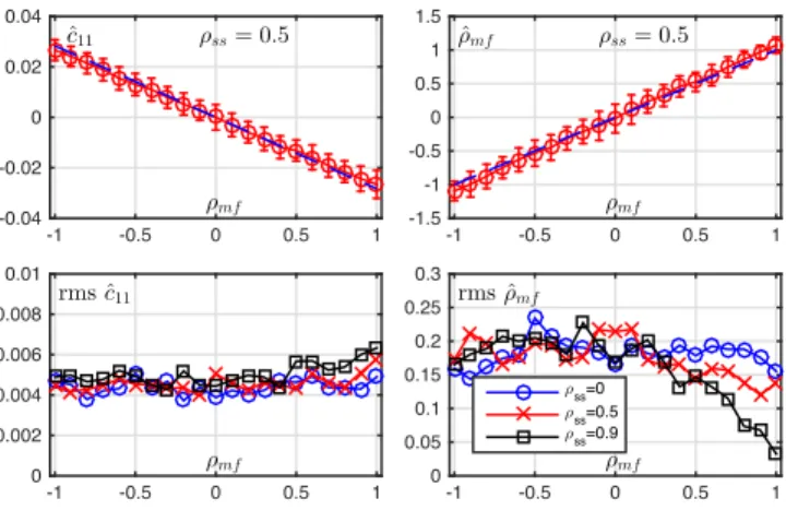
func--1 -0.5 0 0.5 1 -0.04 -0.02 0 0.02 0.04 ˆ c11 ρss= 0.5 ρmf -1 -0.5 0 0.5 1 -1.5 -1 -0.5 0 0.5 1 1.5 ˆ ρmf ρss= 0.5 ρmf -1 -0.5 0 0.5 1 0 0.002 0.004 0.006 0.008 0.01 rms ˆc11 ρmf -1 -0.5 0 0.5 1 0 0.05 0.1 0.15 0.2 0.25 0.3 rms ˆρmf ρmf ρss=0 ρss=0.5 ρss=0.9
Fig. 2. Estimates for bivariate parameters c11(left column) and ⇢mf (right column) as a function of multifractal correlation ⇢mf. Top row: averages (red circles) and standard deviations (error bars) and theoretical values (blue dashed lines) for ˆc11and ˆ⇢mffor ⇢ss= 0.5. Bottom row: root-mean-squared-error values for ⇢ss2 {0, 0.5, 0.9} (blue circles, red crosses, black squares, respectively).
tion of ⇢mf, for a fixed value ⇢ss= 0. It shows that estimation per-formance does not depend on the actual value of ⇢mf. Similar plots, not show here for space reasons, show that estimation performance is also independent of ⇢ss. This indicates that, as expected, estimation performance for univariate multifractal parameters is not impacted by the point dependence structure of the bivariate multivariate pro-cess. For further results on univariate parameters as a function of parameter value, see, e.g., [3].
Bivariate parameters. To investigate the estimation performance for the parameters related to the bivariate dependence structure, let us now turn to ˆc11. Moreover, we propose to study the following nat-ural estimator for the multifractal correlation ⇢mf, cf. (7), defined as
ˆ
⇢mf = ˆc11/p|ˆc20ˆc02|,
where the absolute values are introduced to prevent from negative values under the square root, spuriously induced due to the estima-tion variability for small values of c20 and c02. Fig. 2 (top row) shows averages and standard deviations of ˆc11and ˆ⇢mfas functions of ⇢mf (for ⇢ss = 0.5) and indicates that estimates closely repro-duce the theoretical values c11and ⇢mf and are very satisfactory. Fig. 2 (bottom row) further studies root-mean-squared-error (rms) values for ˆc11and ˆ⇢mf as a function of ⇢mf, for several values of ⇢ss. It leads to conclude that the estimation performance does not depend on ⇢ss, except for a drop in variance observed for ˆ⇢mf for large values of ⇢ssand ⇢mf. Overall, these results indicate that the proposed procedure yields relevant and robust estimates for the bi-variate parameters c11and ⇢mf, with estimation performance largely independent of ⇢ssand ⇢mf.
4.3. Intuitions beyond bivariate multifractal spectra
The Pearson correlation coefficient is a classical tool to assess de-pendence amongst data components. Here we illustrate that the pro-posed bivariate multifractal framework permits to model and analyse dependence beyond the correlation coefficient. Specifically, we de-sign b-MRW with Pearson correlation ⇢bM RW = 0, which is easily achieved by setting ⇢ss = 0, and vary the value for ⇢mf.
Conse--1 -0.5 0 0.5 1 × 10⁻³ -5 0 5 ˆ ρbM RW ρss= 0 ρmf -1 -0.5 0 0.5 1 -1.5 -1 -0.5 0 0.5 1 1.5 ˆ ρmf ρss= 0 ρmf
Fig. 3. Pearson correlation coefficients ˆ⇢bM RW (left) and multifrac-tal correlation ˆ⇢mf(right) as a function of ⇢mffor ⇢ss= 0; shown are averages (red circles), standard deviations (error bars) and theo-retical values (blue dashed lines)
quently, for ⇢mf 6= 0, the process components are strictly uncorre-lated but dependent.
Fig. 3 plots averages and standard deviations of estimates ˆ
⇢bM RW and ˆ⇢mf as a function of ⇢mf. It shows that, indeed, the Pearson correlation coefficient ˆ⇢bM RW ' 0 for ⇢mf 2 [ 1, 1], hence it is completely blind to the dependence between the pro-cess components. In contrast, the multifractal correlation ˆ⇢mf =
ˆ
c11/p|ˆc20ˆc02| provides excellent estimates for ⇢mf and unam-biguously reveals the dependence beyond second statistical order, even for modest values for the correlation |⇢mf|.
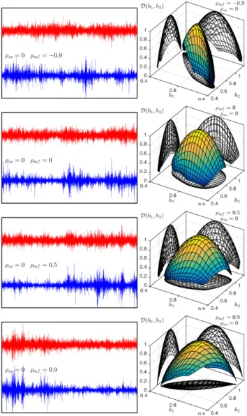
These situations are further illustrated in Fig. 4, which plots several examples of sample path trajectories (left column) with common univariate parameters and ⇢ss = 0, yet different ⇢mf 2 { 0.9, 0, 0.5, 0.9} (from top to bottom), together with the corre-sponding bivariate multifractal spectra estimated using (4) (right column, averages over 100 realizations). In the case ⇢mf = 0, the multifractal spectrum is supported on an ellipse whose main axes are aligned with the h1 and h2 axes, and whose widths are controlled directly and independently by c02and c20. In this case, the process components are not only uncorrelated but also independent. For ⇢mf = 0.5and, a forteriori, in the case ⇢mf = 0.9, the support of D(h) is rotated towards the diagonal and concentrates along the main axis of a slim, rotated ellipse, clearly revealing a situation departing from the previous case without higher-order dependence. Visual investigation of the sample path trajectories indicates that in this situation, the magnitudes of the process components tend to expand and shrink simultaneously. Finally, when ⇢mf = 0.9, the support of D(h) is rotated towards the anti-diagonal, and one sample trajectory tends to expand at time instances where the other one shrinks, and vice versa. Note that the projections of D(h) on the h1= 0and h2= 0planes, respectively, have the same position, shape and width since these are entirely controlled by the univariate parameters (c10, c01, c20, c02)only, which are the same in all cases. To conclude, all these results show that while the traditional cor-relation measure indicates no corcor-relation amongst the two compo-nents, ˆ⇢bM RW ' 0, the shape of the multifractal spectrum, that can in this simple pedagogical model process be summarized by the mul-tifractal correlation ⇢mf, captures statistical dependencies amongst components beyond Pearson correlation and second order statistics. These dependencies are thus involving the entire joint statistical dis-tribution of the bivariate process. In the multifractal setting, these dependencies take the form of joint occurrences of local or transient singularities of same strengths, or equivalently, related values for the H¨older exponents (h1(t), h2(t))for each time location t.
Fig. 4. Bivariate sample paths of b-MRW (left column) and esti-mates of D(h) (right column, averages over 100 realizations) for ⇢ss= 0and ⇢mf 2 { 0.9, 0, 0.5, 0.9} (from top to bottom).
5. CONCLUSIONS AND PERSPECTIVES
The present work defined a wavelet leader based bivariate multifrac-tal formalism for the estimation of the joint multifracmultifrac-tal spectrum of pairs of time series. The estimation performance for univariate and bivariate multifractal parameters was assessed, studied and vali-dated numerically for bivariate MRW, a bivariate extension of a sim-ple yet versatile stochastic multifractal model. We provided intuitive interpretations and illustrations for the essence of the wealth of in-formation that is captured by the bivariate multifractal spectrum. In particular, it was shown that it permits to model and quantify local and transient dependencies involving the entire joint statistical distri-bution of the random vectors defining the bivariate process, beyond second statistical order and hence correlation analysis, that can be interpreted in terms of pointwise inter-related regularity exponents. The proposed joint multifractal modeling and analysis framework extends beyond bivariate time series and to the use of p-leaders and p-exponents as multiresolution quantities and regularity exponents.
6. REFERENCES
[1] A. Chhabra, C. Meneveau, R. V. Jensen, and K. R. Sreenivasan, “Direct determination of the singularity spectrum and its appli-cation to fully developed turbulence,” Phys. Rev. A, vol. 40, no. 9, pp. 5284, 1989.
[2] S. Jaffard, “Wavelet techniques in multifractal analysis,” in Fractal Geometry and Applications: A Jubilee of Benoˆıt Man-delbrot, M. Lapidus and M. van Frankenhuijsen, Eds., Proc. Symposia in Pure Mathematics. 2004, vol. 72(2), pp. 91–152, AMS.
[3] H. Wendt, P. Abry, and S. Jaffard, “Bootstrap for empirical multifractal analysis,” IEEE Signal Proc. Mag., vol. 24, no. 4, pp. 38–48, 2007.
[4] K. Kiyono, Z. R. Struzik, N. Aoyagi, and Y. Yamamoto, “Mul-tiscale probability density function analysis: non-Gaussian and scale-invariant fluctuations of healthy human heart rate,” IEEE Trans. Biomed. Eng., vol. 53, no. 1, pp. 95–102, Jan. 2006. [5] P. Ciuciu, G. Varoquaux, P. Abry, S. Sadaghiani, and A.
Klein-schmidt, “Scale-free and multifractal time dynamics of fMRI signals during rest and task,” Front. Physiol., vol. 3, June 2012. [6] M. Doret, H. Helgason, P. Abry, P. Gonc¸alv`es, C. Gharib, and P. Gaucherand, “Multifractal analysis of fetal heart rate vari-ability in fetuses with and without severe acidosis during la-bor,” Am. J. Perinatol., vol. 28, no. 4, pp. 259–266, 2011. [7] F. Wang, Z.-S. Li, and J.-W. Li, “Local multifractal detrended
fluctuation analysis for non-stationary image’s texture segmen-tation,” Applied Surface Science, vol. 322, pp. 116–125, 2014. [8] R. Fontugne, P. Abry, K. Fukuda, D. Veitch, K. Cho, P. Borgnat, and H. Wendt, “Scaling in internet traffic: a 14 year and 3 day longitudinal study, with multiscale analyses and random projections,” IEEE/ACM T. Networking, vol. 25, no. 4, 2017.
[9] B. B. Mandelbrot, “Intermittent turbulence in self-similar cas-cades: divergence of high moments and dimension of the car-rier,” J. Fluid Mech., vol. 62, pp. 331–358, 1974.
[10] A. Johansen and D. Sornette, “Finite-time singularity in the dynamics of the world population, economic and financial in-dices,” Physica A, vol. 294, pp. 465–502, 2001.
[11] G. Valenza, H. Wendt, K. Kiyono, J. Hayano, E. Watanabe, Y. Yamamoto, P. Abry, and R. Barbieri, “Multifractal point-process heartbeat dynamics: a congestive heart failure survivor prediction study,” IEEE T. Biomedical Engineering, 2018, in press.
[12] C. Meneveau, K.R. Sreenivasan, P. Kailasnath, and M.S. Fan, “Joint multifractal measures - theory and applications to turbu-lence,” Phys. Rev. A, vol. 41, no. 2, pp. 894–913, 1990. [13] T. Lux, “Higher dimensional multifractal processes: A GMM
approach,” Journal of Business and Economic Statistics, vol. 26, pp. 194–210, 2007.
[14] J. F. Muzy, E. Bacry, and A. Arneodo, “Multifractal formalism for fractal signals: The structure-function approach versus the wavelet-transform modulus-maxima method,” Phys. Rev. E, vol. 47, no. 2, pp. 875, 1993.
[15] R. Leonarduzzi, H. Wendt, S. G. Roux, M. E. Torres, C. Melot, S. Jaffard, and P. Abry, “p-exponent and p-leaders, Part II: Multifractal analysis. Relations to Detrended Fluctuation Anal-ysis,” Physica A, vol. 448, pp. 319–339, 2016.
[16] E. Bacry, J. Delour, and J.-F. Muzy, “Multifractal random walk,” Phys. Rev. E, vol. 64: 026103, 2001.
[17] E. Bacry, J. Delour, and J. F. Muzy, “A multivariate multi-fractal model for return fluctuations,” arXiv preprint cond-mat/0009260, 2000.
[18] S. Jaffard, S. Seuret, H. Wendt, R. Leonarduzzi, S. Roux, and P. Abry, “Multivariate multifractal analysis,” Applied and Computational Harmonic Analysis, 2018, in press.
[19] S. Mallat, A Wavelet Tour of Signal Processing, Academic Press, San Diego, CA, 1998.
[20] B. Castaing, Y. Gagne, and M. Marchand, “Log-similarity for turbulent flows,” Physica D, vol. 68, no. 3-4, pp. 387–400, 1993.
[21] G. Samorodnitsky and M. Taqqu, Stable non-Gaussian random processes, Chapman and Hall, New York, 1994.
[22] G. Didier and V. Pipiras, “Integral representations and proper-ties of operator fractional Brownian motions,” Bernoulli, vol. 17, no. 1, pp. 1–33, 2011.
[23] H. Helgason, V. Pipiras, and P. Abry, “Fast and exact synthesis of stationary multivariate Gaussian time series using circulant embedding,” Signal Proc., vol. 91, no. 5, pp. 1123–1133, 2011.