Toward a numerical predictive method based on fatigue analysis for droplet impingement erosion

HAL Id: tel-02063381

https://tel.archives-ouvertes.fr/tel-02063381

Submitted on 11 Mar 2019

HAL is a multi-disciplinary open access

archive for the deposit and dissemination of sci-entific research documents, whether they are pub-lished or not. The documents may come from teaching and research institutions in France or

L’archive ouverte pluridisciplinaire HAL, est destinée au dépôt et à la diffusion de documents scientifiques de niveau recherche, publiés ou non, émanant des établissements d’enseignement et de recherche français ou étrangers, des laboratoires

Guillaume Coudouel

To cite this version:

Guillaume Coudouel. Toward a numerical predictive method based on fatigue analysis for droplet impingement erosion. Fluids mechanics [physics.class-ph]. Université de Lyon, 2017. English. �NNT : 2017LYSEI101�. �tel-02063381�

N° d’ordre NNT : 2017LYSEI101

THESE de DOCTORAT DE L’UNIVERSITE DE LYON

opérée au sein de

l’Institut National des Sciences Appliquées de Lyon

Ecole Doctorale

ED162

Mécanique, Energétique, Génie Civil, Acoustique

Spécialité/ discipline de doctorat

:

Génie Mécanique

Soutenue publiquement le 26/10/2017, par :

Guillaume Coudouel

Toward a numerical predictive method

based on fatigue analysis for droplet

impingement erosion

Devant le jury composé de :

C. GARDIN Professeur des Universités ISAE-ENSMA Présidente de jury V. FAUCHER Expert senior HDR CEA Cadarache Rapporteur

H. MAITOURNAM Professeur des Universités ENSTA ParisTech Rapporteur

J.-C. MARONGIU Docteur ANDRITZ Hydro Examinateur

E. SALLÉ Professeur des Universités INSA de Lyon Examinatrice A. COMBESCURE Professeur des Universités INSA de Lyon Directeur de thèse

CHIMIE

CHIMIE DE LYON

http://www.edchimie-lyon.fr

Sec : Renée EL MELHEM Bat Blaise Pascal 3e _etage

[email protected] Insa : R. GOURDON

M. Stéphane DANIELE

Institut de Recherches sur la Catalyse et l'Environnement de Lyon IRCELYON-UMR 5256

Équipe CDFA

2 avenue Albert Einstein 69626 Villeurbanne cedex [email protected] E.E.A. ELECTRONIQUE, ELECTROTECHNIQUE, AUTOMATIQUE http://edeea.ec-lyon.fr Sec : M.C. HAVGOUDOUKIAN [email protected] M. Gérard SCORLETTI

Ecole Centrale de Lyon 36 avenue Guy de Collongue 69134 ECULLY Tél : 04.72.18 60.97 Fax : 04 78 43 37 17 [email protected] E2M2 EVOLUTION, ECOSYSTEME, MICROBIOLOGIE, MODELISATION http://e2m2.universite-lyon.fr

Sec : Sylvie ROBERJOT Bât Atrium - UCB Lyon 1 04.72.44.83.62 Insa : H. CHARLES

[email protected]

M. Fabrice CORDEY

CNRS UMR 5276 Lab. de géologie de Lyon Université Claude Bernard Lyon 1 Bât Géode

2 rue Raphaël Dubois 69622 VILLEURBANNE Cédex Tél : 06.07.53.89.13 cordey@ univ-lyon1.fr EDISS INTERDISCIPLINAIRE SCIENCES- SANTE http://www.ediss-lyon.fr

Sec : Sylvie ROBERJOT Bât Atrium - UCB Lyon 1 04.72.44.83.62 Insa : M. LAGARDE

[email protected]

Mme Emmanuelle CANET-SOULAS

INSERM U1060, CarMeN lab, Univ. Lyon 1 Bâtiment IMBL

11 avenue Jean Capelle INSA de Lyon 696621 Villeurbanne Tél : 04.72.68.49.09 Fax :04 72 68 49 16 [email protected] INFOMATHS INFORMATIQUE ET MATHEMATIQUES http://infomaths.univ-lyon1.fr

Sec :Renée EL MELHEM Bat Blaise Pascal, 3e é_tage Tél : 04.72. 43. 80. 46 Fax : 04.72.43.16.87 [email protected] M. Luca ZAMBONI Bâtiment Braconnier 43 Boulevard du 11 novembre 1918 69622 VILLEURBANNE Cedex Tél :04 26 23 45 52 [email protected] Matériaux MATERIAUX DE LYON http://ed34.universite-lyon.fr

Sec : Marion COMBE

Tél:04-72-43-71-70 –Fax : 87.12 Bat. Direction [email protected] M. Jean-Yves BUFFIERE INSA de Lyon MATEIS

Bâtiment Saint Exupéry 7 avenue Jean Capelle 69621 VILLEURBANNE Cedex

Tél : 04.72.43 71.70 Fax 04 72 43 85 28 [email protected]

MEGA

MECANIQUE, ENERGETIQUE, GENIE CIVIL, ACOUSTIQUE

http://mega.universite-lyon.fr

Sec : Marion COMBE

Tél:04-72-43-71-70 –Fax : 87.12 Bat. Direction [email protected] M. Philippe BOISSE INSA de Lyon Laboratoire LAMCOS Bâtiment Jacquard 25 bis avenue Jean Capelle 69621 VILLEURBANNE Cedex Tél : 04.72 .43.71.70 Fax : 04 72 43 72 37 [email protected] ScSo ScSo* http://recherche.univ-lyon2.fr/scso/

Sec : Viviane POLSINELLI Brigitte DUBOIS Insa : J.Y. TOUSSAINT Tél :04 78 69 72 76 [email protected] M. Christian MONTES Université Lyon 2 86 rue Pasteur 69365 LYON Cedex 07 [email protected]

Cette th`ese d´ebut´ee en octobre 2014 a ´et´e r´ealis´ee dans le cadre du projet europ´een FP7 / 2007-2013 sous la convention de subvention 608393, nomm´e PrEDHyMa. Elle fut le fruit d’une collaboration entre le Laboratoire de M´ecanique des Contacts et des Structures (LaMCoS) de l’Institut National de Sciences Appliqu´ee (INSA) de Lyon, le Laboratoire de M´ecanique des Fluides et d’Acoustique (LMFA) de l’ ´Ecole Centrale de Lyon (ECL) et la soci´et´e ANDRITZ Hydro. Je tiens donc `a remercier en premier lieu l’ensemble des partenaires m’ayant fourni un cadre de travail propice `a la r´ealisation de ce travail durant ces trois ann´ees.

Je remercie MM. Vincent Faucher et Habibou Maitournam pour avoir accept´e d’ˆetre rapporteurs de mon travail, Mme. Catherine Gardin pour avoir accept´e de pr´esider ce jury, ainsi que les examinateurs : M. Jean-Christophe Marongiu et Mme. Emmanuelle Sall´e.

Je tiens `a adresser mes plus chaleureux remerciements `a M. Alain Combescure, mon directeur de th`ese, qui s’est montr´e attentif, bienveillant, compr´ehensif, tol´erant, atten-tionn´e, patient, encourageant, extrˆemement r´eactif et toujours disponible. Grˆace `a ses pr´ecieuses connaissances, son exp´erience et son recul, il m’a judicieusement aiguill´e dans ma progression tout au long de cette aventure longue de trois ann´ees. En effet, chaque r´eunion de suivi s’est r´ev´el´ee stimulante et me motivait dans la poursuite du travail, mˆeme en ´etant bloqu´e, puisque les discussions menaient `a des solutions claires et des d´emarches efficaces, le tout me permettant de m’approprier le sujet. Je consid`ere que l’avoir eu comme Maˆıtre fut un immense privil`ege et une chance inou¨ıe.

Je remercie particuli`erement M. Jean-Christophe Marongiu, chef de l’´equipe Turbine Physicschez ANDRITZ Hydro, pour avoir propos´e et mis en place ce projet et nous avoir encadr´es, pour sa disponibilit´e ainsi que ses explications claires concernant la dynamique des fluides num´erique (notamment la m´ethode SPH) et le temps pass´e `a nous aider `a maitriser les outils num´eriques n´ecessaires.

Je remercie en outre les autres doctorants du projet PrEDHyMa, avec qui j’ai eu de nombreux ´echanges fructueux et scientifiquement pertinents : Wiebke Boden, Saira Pineda et tout particuli`erement Jorge Nu˜nez, v´eritable ami, d’une grande aide, qui a g´en´ereusement partag´e ses connaissances dans l’utilisation du shell sous Linux et des langages C et ForTran.

Je souhaite aussi exprimer ma gratitude envers M. Etienne Parkinson, Technical Ma-nager et chef du d´epartement R&D chez ANDRITZ Hydro Vevey qui m’a permis de travailler dans un environnement favorable `a l’accomplissement de ce travail de recher-che, et aussi envers les autres collaborateurs du d´epartement R&D d’ANDRITZ Vevey et Villeurbanne qui m’ont chaleureusement accueilli lors de cette aventure : les deux Nico-las, Steven, Adrien, H´el`ene, Matthias, Martin, Magdalena, Ralph, ansi que Herv´e pour son aide et ses judicieux conseils en programmation (particuli`erement en C) ainsi que sur CMake.

Yannick, Fatima, Guillaume, Salvatore, Corentin, Wenfeng, Yancheng, Kevin, Marie, Lv, ainsi qu’`a ceux des nouvelles ´equipes MIMESIS et MULTIMAP : Tristan, Thibaut, Pierre, Matthieu, Arthur, Thomas, Zhi Kang, et tous ceux des autres salles et ´etages...

Enfin, une grande part de ma r´eussite revient `a mes parents qui m’ont encourag´e et soutenu depuis toujours dans mes r´ealisations, et particuli`erement durant cette “odyss´ee”.

Le but du travail pr´esent´e est la compr´ehension puis la simulation num´erique des m´ecanismes d’´erosion des augets de turbine Pelton par impacts r´ep´et´es de gouttes d’eau dans le but de pr´edire la dur´ee de vie des composants. Tout d’abord, les ph´enom`enes de propagation d’ondes dans les milieux fluide et solide sont ´etudi´es. Cela permet de mettre en lumi`ere l’´evolution temporelle et la distribution spatiale des pressions de con-tact, et l’apparition de microjets par ´ejection supersonique du fluide au contact. Les ´etudes exp´erimentales de l’´erosion par gouttes d’eau traduisent un dommage bas´e sur la fissuration par fatigue. Des simulations num´eriques en dynamique rapide coupl´ees fluide-structure sont alors effectu´ees. Le domaine solide est discr´etis´e par la M´ethode des ´el´ements Finis (MEF), et le domaine fluide par la m´ethode Smoothed Particle Hydrody-namics(SPH), qui est une m´ethode particulaire (sans maillage) particuli`erement adapt´ee aux grandes distorsions et au suivi des surfaces libres. L’analyse des ´etats de contrain-tes vient corroborer la nature cyclique de l’endommagement. La simulation d’´erosion est alors r´ealis´ee `a l’aide de crit`eres de fatigue multiaxiaux. Le choix se porte vers un premier crit`ere g´en´eral de l’American Society of Mechanical Engineers (ASME), utili-sant les valeurs principales des diff´erences de contraintes au cours du temps. Le second choix concerne un crit`ere `a plan critique : le crit`ere de Dang Van 2. Il traite s´epar´ement la contrainte hydrostatique et le cisaillement altern´e maximal local. Ces crit`eres permet-tent de d´efinir les r´egions ´erod´ees du solide au bout d’un nombre d’impact donn´e, ce qui fait de cette d´emarche une m´ethode pr´edictive. Une ´etude param´etrique pour diff´erentes tailles de gouttes et vitesses d’impact est ensuite r´ealis´ee, puis on ´evalue l’influence de la pr´esence d’une couche de coating.

M

OTS CLES

´

:

Impact de goutte, ´Erosion, Couplage fluide-structure, Fatigue, ´El´ements Finis, Smoothed Particle Hydrodynamics.

The goal of this work is the comprehension and the numerical simulation of erosion caused by repeated droplet impact on Pelton turbine buckets, to predict the lifetime of these components. First, waves propagation phenomenon inside fluid and solid domains are presented, which allows determining the time evolution and spatial distribution of con-tact pressure, and the birth of lateral microjets by supersonic ejection of the fluid on the contact. Experimental studies of erosion by droplet impact highlight a fatigue cracking-based erosion mechanism. Then, coupled FSI computation are performed. The solid subdomain is discretized by the Finite Element Method (FEM), and the fluid subdomain by the Smoothed Particle Hydrodynamics (SPH), which is a particle method (meshless) effectively recommended for large distortions and free surface tracking. Stress analysis confirms the cyclic nature of the damage mechanism, and erosion simulation is perfor-med using multiaxial fatigue criteria. The first selected criterion is a general one from the American Society of Mechanical Engineers (ASME) using principal values of stress differences over time. The second one is the Dang van 2 criterion, belonging to the family of critical plane criteria. This criterion considers separately the effects due to hydrostatic stress on one hand, and the ones induced by maximum local shear on the other. These two criteria are used to building the equivalent eroded zones of the solid subdomain for a gi-ven number of impacts, which allows to qualify this procedure as a predictive predictive. Finally, a parametric study for different droplet sizes and velocity is computed, and the effects of a coating layer are investigated.

K

EYWORDS

:

Droplet impact, Erosion, Fluid-structure interaction, Fatigue, Finite Element Method, Smoothed Particle Hydrodynamics.

Contents i

List of Figures v

List of Tables xi

Nomenclature 1

Introduction 5

1 Physical phenomenon of droplet impact erosion 11

1.1 Droplet impact . . . 12

1.1.1 Waves propagation . . . 12

1.1.2 Contact pressure . . . 13

1.1.3 Jetting . . . 19

1.1.4 Cavitation . . . 21

1.2 Erosion mechanism : experimental approach . . . 23

1.2.1 Test rigs . . . 23

1.2.2 Macroscopic scale . . . 24

1.2.3 Material science based models . . . 30

1.2.4 Coating . . . 33

1.3 Conclusion on the mechanism of droplet impact erosion . . . 38

2 Numerical methods for droplet impact 41 2.1 Strong form of continuum mechanics . . . 43

2.1.1 Different configurations in continuum mechanics . . . 43

2.1.2 Conservations laws in continuum mechanics . . . 43

2.1.3 The Solid sub-domain . . . 45

2.1.4 The fluid sub-domain . . . 51

2.1.5 Coupling conditions . . . 52

2.2 Weak form and numerical discretization . . . 53

2.2.1 FEM for solid sub-domain . . . 53

2.2.2 SPH for fluid sub-domain . . . 59

2.2.4 FSI coupling . . . 65

2.3 Numerical simulation of droplet impact phenomenon . . . 66

2.3.1 Model features . . . 66

2.3.2 Convergence of fluid computation . . . 67

2.3.3 One-way coupling . . . 76

2.3.4 Two-way coupling . . . 78

2.4 Conclusion on numerical methods for droplet impact . . . 82

3 Fatigue developments 89 3.1 The fatigue phenomenon . . . 91

3.1.1 Introduction . . . 91

3.1.2 Generalities . . . 91

3.1.3 Definition of terms used in fatigue . . . 91

3.1.4 The different fatigue domains . . . 93

3.1.5 The different fatigue loads . . . 94

3.1.6 Conclusion on fatigue phenomenon . . . 95

3.2 Multiaxial fatigue criteria . . . 95

3.2.1 General ASME criterion . . . 95

3.2.2 Specific criteria . . . 96

3.3 Choice of fatigue criterion . . . 100

3.3.1 Presentation of Dang Van criterion [DAN 71, DAN 84] . . . 101

3.3.2 Determination of the critical plane . . . 102

3.3.3 Second version of Dang Van criterion [DAN 89] . . . 103

3.4 Fatigue erosion predicting tool . . . 104

3.4.1 General procedure . . . 104

3.4.2 Protocol for stress amplitude calculation . . . 106

3.4.3 Procedure for new FSI boundary determination . . . 107

3.5 Conclusion on fatigue developments . . . 108

4 Prediction of damage due to repeated droplets impacts 111 4.1 Features and assumptions . . . 112

4.2 Results for non-coated surface . . . 114

4.2.1 Results of parametric analysis . . . 114

4.2.2 Solid mesh convergence checking . . . 120

4.3 Adding the coating layer . . . 121

4.3.1 Effects on transient evolution . . . 122

4.3.2 Effects on fatigue resistance and lifetime . . . 124

4.3.3 Discussion about results and limitations . . . 127

4.4 Conclusion on prediction of damage due to droplets impacts . . . 127

General conclusion & perspectives 139

Bibliography 157

R´esum´e ´etendu 175

0.0 Introduction . . . 175

0.1 Explication physique de l’´erosion par choc de goutte . . . 175

0.1.1 Physique de l’impact de goutte . . . 176

0.1.2 M´ecanisme d’´erosion . . . 178

0.2 Simulation num´erique de l’´erosion par choc de goutte . . . 179

0.2.1 Caract´eristiques du mod`ele num´erique . . . 180

0.2.2 Equations r´egissant le comportement des sous-domaines . . . 181

0.2.3 Convergence et impact sur mur rigide . . . 181

0.2.4 Simulation par couplage faible . . . 182

0.2.5 Simulation par couplage fort . . . 182

0.3 Analyse en fatigue et pr´ediction du dommage . . . 184

0.3.1 Proc´edure d’´erosion . . . 185

0.3.2 Crit`eres de fatigues utilis´es . . . 186

0.3.3 Etude param´etrique du mod`ele sans coating . . . 188´

0.3.4 Ajout de la couche de coating . . . 189

1 A six-injector vertical-axis Pelton runner . . . 7 2 Erosion damage visible on a Pelton turbine bucket at the end of its

functi-onal lifetime . . . 8 1.1 Shock front and highly compressed volume on early time of droplet impact 12 1.2 Geometrical construction of wave front with Huygens-Fresnel principle . 13 1.3 Time evolution of density during the droplet impact . . . 14 1.4 Different types of waves involved when a water droplet impacts an elastic,

isotropic, and homogeneous solid body . . . 15 1.5 Water-hammer pressure vs. impact velocity for water droplet on rigid target 16 1.6 Ratio between water hammer edge and droplet radius vs. impact velocity

for water droplet on rigid target . . . 17 1.7 Spatial distribution of contact pressure for several times after impact (R =

0.1 mm, V = 500 m.s−1) . . . 18 1.8 Map of high pressure duration as a function of droplet radius and impact

velocity for water droplet on rigid target . . . 20 1.9 Birth of lateral microjets . . . 21 1.10 Radial velocity and density distribution on the contact zone when jetting . 21 1.11 Steps of near-side cavitation formation . . . 22 1.12 Impact of 10 mm diameter water drop by a metal slider at a velocity of

110 m.s−1 . . . 23 1.13 Principles scheme of PJET . . . 24 1.14 Example of a small, relatively low-speed, rotating disk-and-jet repetitive

impact apparatus . . . 24 1.15 Example of a large, high-speed, rotating arm-and-spray distributed impact

apparatus . . . 25 1.16 Typical erosion curve . . . 26 1.17 Normalized volume loss of X20Cr13 as a function of droplet impact angle

with impact speed V = 488 m.s−1 . . . 27 1.18 Erosion behaviour of X20Cr13 at different droplet sizes tested at the

im-pact velocity of 488 m.s−1 . . . 28 1.19 Erosion behaviour of 12%Cr steel at different impact velocities for a

1.20 Grain ruptures on the initial surface of H300 after 50’000 impacts at

im-pact velocity V = 225 m.s−1 . . . 30

1.21 Fatigue defects observed on H300 after 5 million and 10 million impacts, at impact velocity V = 225 m.s−1 . . . 31

1.22 Cross section of eroded stainless steel at different magnification, at impact velocity V = 225 m.s−1 . . . 31

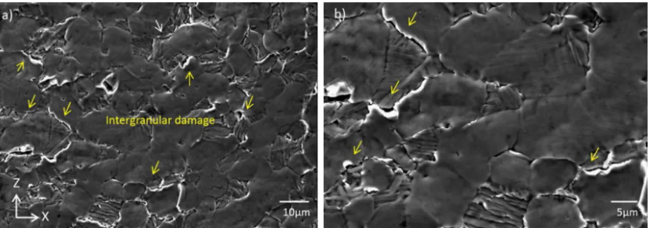
1.23 Intergranular damage observed on Ti-6Al-4V, at impact velocity V = 350 m.s−1 . . . 32

1.24 Born of triple junctions an microvoids on Ti-6Al-4V, at impact velocity V = 350 m.s−1 . . . 32

1.25 Grain ejection, striation inside crater and slip bands on Ti-6Al-4V, at im-pact velocity V = 350 m.s−1 . . . 33

1.26 Stress wave propagation observed on γ-TiAl surface . . . 34

1.27 Intergranular and intragranular cracking in γ-TiAl . . . 34

1.28 Triple split resulting from grain pulled-out in γ-TiAl . . . 35

1.29 The two modes of intragranular fractures in γ-TiAl . . . 35

1.30 Areas sensitive to cracking in Pelton buckets . . . 36

1.31 HVOF coating on Pelton buckets . . . 36

1.32 Schematic diagram of the high velocity oxy-fuel spray process (HVOF) . 37 1.33 WC 10Co 4Cr coating materials . . . 37

1.34 Section of a coated bucket . . . 37

1.35 Eroded surfaces of Pelton runner without coating and with SHXTM coa-ting after operation . . . 38

2.1 The normal vectors for each sub-domain at the fluid-structure interface . . 53

2.2 The solid domain Ωs discretized by a Lagrangian mesh under two types of boundary conditions . . . 54

2.3 Kernel approximation with the smoothing kernel function . . . 61

2.4 Representation and dimensions of the numerical model . . . 67

2.5 Dynamic system and time evolution of load force . . . 69

2.6 Distribution of probes in 2-D model . . . 71

2.7 Distribution of probes in 3-D model . . . 71

2.8 Impulse distribution of 3-D computation . . . 72

2.9 Comparison of impulse distribution between 2-D and 3-D models . . . . 73

2.10 Comparison of impulse distribution between full and symmetric models . 74 2.11 Different models for truncation . . . 74

2.12 Comparison of impulse distribution between full and truncated models . . 75

2.13 Comparison of impulse distribution for different particle sizes . . . 76

2.14 Contact pressure on rigid wall . . . 78

2.15 Pressure field inside the droplet at t = 150 ns after impact with ∆x = 6 · 10−7m . . . 78

2.17 Pressure inside fluid, hydrostatic and Von Mises stresses inside solid for

several times after impact . . . 80

2.18 Time evolution of hydrostatic and Von Mises stresses at x = 0.1425 mm, z= −2.5 µm . . . 82

2.19 Time evolution of stress triaxiality at x = 0.1425 mm, z = −2.5 µm . . . . 83

2.20 Signed Von Mises Stress inside solid and pressure inside fluid at jetting time 84 2.21 Time evolution of principal stresses at x = 0.1425 mm, z = −2.5 µm . . . 85

2.22 Time evolution of principal stresses ratios at x = 0.1425 mm, z = −2.5 µm 86 2.23 Time evolution of principal angle at x = 0.1425 mm, z = −2.5 µm . . . . 87

3.1 Example of sinusoidal load cycles . . . 92

3.2 S-N diagram and different fatigue domains . . . 94

3.3 Decomposition of stress vector in basis linked to physical plane . . . 98

3.4 Definition of terms related to normal stress . . . 98

3.5 Definition of terms related to tangential stress . . . 100

3.6 Endurance domain and two typical load paths . . . 102

3.7 Procedure for erosion simulation . . . 105

3.8 S-N diagram with upper stress and lower cycle limits . . . 105

3.9 Procedure for calculation of stress amplitude for the ASME criterion . . . 107

3.10 Procedure for calculation of stress amplitude for the Dang Van 2 criterion 108 3.11 Example of mesh with eroded elements and modification of FSI interface 109 4.1 Representation and dimensions of numerical model involving coating layer 113 4.2 Raw and coating materials behaviour curves : Traction curve and S-N diagram . . . 113

4.3 Stress amplitude inside solid according to ASME criterion on left and Dang Van 2 criterion on right, and pressure inside fluid at t = 460 ns after impact for the case (φ = 1 mm,V = 100 m.s−1) . . . 115

4.4 Number of cycles to failure according to ASME criterion on left and Dang Van 2 criterion on right, at t = 460 ns after impact for the case (φ = 1 mm,V = 100 m.s−1) . . . 116

4.5 Influence of droplet diameter and impact velocity on maximum stress am-plitude according to both criteria . . . 117

4.6 Influence of droplet diameter and impact velocity on minimum number of cycles to failure according to both criteria . . . 117

4.7 Influence of droplet diameter and impact velocity on number of eroded elements according to both criteria for Nlim= 5 · 107cycles . . . 118

4.8 Influence of droplet diameter and impact velocity on erosion depth accor-ding to both criteria for Nlim= 5 · 107cycles . . . 119

4.9 Fatigue function and non-eroded elements for Nlim= 5 · 107 cycles ac-cording to both criteria, at t = 460 ns after impact for the case (φ = 0.5 mm,V = 100 m.s−1) . . . 120

4.10 Fatigue function and non-eroded elements for Nlim= 5 · 107 cycles ac-cording to both criteria, at t = 460 ns after impact for the case (φ = 0.5 mm,V = 200 m.s−1) . . . 121 4.11 Fatigue function and non-eroded elements for Nlim= 5 · 107cycles

accor-ding to both criteria, at t = 460 ns after impact for the case (φ = 1 mm,V = 100 m.s−1) . . . 122 4.12 Fatigue function and non-eroded elements for Nlim= 5 · 107cycles

accor-ding to both criteria, at t = 460 ns after impact for the case (φ = 1 mm,V = 200 m.s−1) . . . 123 4.13 Fatigue function and non-eroded elements for Nlim= 5 · 107cycles

accor-ding to both criteria, at t = 460 ns after impact for the case (φ = 2 mm,V = 100 m.s−1) . . . 124 4.14 Fatigue function and non-eroded elements for Nlim= 5 · 107cycles

accor-ding to both criteria, at t = 460 ns after impact for the case (φ = 2 mm,V = 200 m.s−1) . . . 125 4.15 Dang Van 2 stress amplitude for standard mesh and refined one in the

hig-hest stress region, at t = 460 ns after impact for (φ = 1 mm,V = 100 m.s−1)125 4.16 Dang Van 2 fatigue function and non-eroded elements for Nlim= 107

cy-cles using standard mesh and refined one in eroded region, at t = 460 ns after impact for (φ = 1 mm,V = 100 m.s−1) . . . 126 4.17 Comparison of hydrostatic stress between the pure basic material and the

coated one at different frames for the case (φ = 1 mm,V = 100 m.s−1) . . 129 4.18 Comparison of Von Mises stress between the pure basic material and the

coated one at different frames for the case (φ = 1 mm,V = 100 m.s−1) . . 130 4.19 Comparison of maximum value of stress amplitude over the mesh

accor-ding to both criteria between the two material configurations for the case (φ = 1 mm,V = 100 m.s−1) . . . 131 4.20 Comparison of minimum value of number of cycles to failure over the

mesh according to both criteria between the two material configurations for the case (φ = 1 mm,V = 100 m.s−1) . . . 132 4.21 Comparison of ASME stress amplitude between pure basic material and

coated one at t = 460 ns after impact for φ = 1 mm and V = 100 m.s−1 . 133 4.22 Comparison of Dang Van 2 stress amplitude between pure basic material

and coated one at t = 460 ns after impact for φ = 1 mm and V = 100 m.s−1134 4.23 Comparison of number of cycles to failure according to ASME criterion

between pure basic material and coated one at t = 460 ns after impact for φ = 1 mm and V = 100 m.s−1 . . . 135 4.24 Comparison of number of cycles to failure according to Dang Van 2

crite-rion between pure basic material and coated one at t = 460 ns after impact for φ = 1 mm and V = 100 m.s−1 . . . 136 4.25 Comparison of fatigue function for Nlim = 3 · 109 cycles according to

ASME criterion between pure basic material and coated one at t = 460 ns after impact for φ = 1 mm and V = 100 m.s−1 . . . 137

4.26 Comparison of fatigue function for Nlim = 3 · 109 cycles according to Dang Van 2 criterion between pure basic material and coated one at t = 460 ns after impact for φ = 1 mm and V = 100 m.s−1 . . . 138 27 Front d’onde et volume comprim´e en d´ebut d’impact . . . 176 28 Formation des microjets lat´eraux . . . 177 29 Dommage par fatigue observ´e sur de l’acier H300 apr`es 5 et 10 millions

d’impacts `a vitesse V = 225 m.s−1 . . . 179 30 Repr´esentation et dimensions du mod`ele num´erique . . . 180 31 Pression de contact sur le mur rigide . . . 183 32 Pression dans le fluide, contraintes hydrostatique et de Mon Mises dans

le solide en diff´erents instants apr`es impact . . . 184 33 Evolution temporelle des contraintes hydrostatique σ´ H et de Von Mises

σVMen x = 0.1425 mm, z = −2.5 µm . . . 185 34 Proc´edure de la simulation d’´erosion . . . 186 35 Fonction de fatigue et ´el´ements non-´erod´es pour Nlim = 5 · 107 cycles

d’apr`es chaque crit`ere, au temps t = 460 ns apr`es impact, pour le cas (φ = 1 mm,V = 100 m.s−1) . . . 190 36 Comparaison de la contrainte de Von Mises entre le mod`ele en acier pur

et celui avec coating en diff´erents instants pour le cas (φ = 1 mm,V = 100 m.s−1) . . . 191 37 Comparaison de la fonction de fatigue pour Nlim= 3 · 109cycles d’apr`es

le crit`ere de Dang Van 2 entre le mod`ele en acier pur et celui avec coating `a t = 460 ns apr`es impact pour φ = 1 mm et V = 100 m.s−1 . . . 192

2.1 Material data for numerical simulations . . . 67 2.2 CPU time for different 2-D fluid models . . . 76 4.1 Material data for raw material and coating . . . 112

The complete list of notations is given in Appendix A.

Subscripts and superscripts

Symbol Description

•i iline component of vector

•i j iline and j column component of matrix •_I, •II, •III Quantities relative to eigenvalues of a matrix

•f Quantity relative to fluid subdomain only •s Quantity relative to solid subdomain only •h Quantity relative to plane normal to h •AS Quantity relative to ASME criterion •DV2 Quantity relative to DV2 criterion

•0 _{Initial value of a quantity at t = 0}

•a Alternate value during load cycle

•am _{Amplitude of signal over load cycle}

•m _{Mean value during load cycle}

•max _{Maximum value during load cycle}

•min _{Minimum value during load cycle}

Scalars

Parameter Description Unit (ISO)

c Sound velocity m.s−1

E Fatigue function

-N Number of cycles to failure

-N_lim Number of cycles to failure lower limit

-p Pressure field Pa

R Droplet radius m

Rjet Radial location of jetting m

t Physical time s V Impact velocity m.s−1 x Radial location m z Vertical location m δi j Kronecker symbol -∆σ Stress range Pa ρ Density kg.m−3

σK Principal stresses with K = I...III Pa

σlim Stress amplitude upper limit Pa

σH Hydrostatic stress Pa

σVM Von Mises stress Pa

φ Droplet diameter m

Vectors

Parameter Description Unit (ISO)

u Displacement field m

v Velocity field m.s−1

X Material or Lagrangian coordinates m

Matrices

Parameter Description Unit (ISO)

1 Identity matrix -s Deviatoric stress Pa ε Strain field -σ Cauchy stress Pa

Operators

Operator Description •> Transposition operator tr (•) Tracing operator · Dot product

: Double dot product

⊗ Tensor product operator

∇ Gradient operator

Acronyms

Name Description

ASME American Society of Mechanical Engineers (criterion)

DV2 or DV2 Dang Van 2 (criterion)

FEM Finite Element Method

FSI Fluid-Structure Interaction

Hydraulic turbines can undergo severe damage during operation, because of low quality water or detrimental flow conditions. Damage induces maintenance costs and power pro-duction losses, and can also endanger safety of installations. Hydropower plants operators and turbine manufacturers are interested in extending overhaul periods by reducing da-mage intensity and protecting turbine components with surface treatments, but accurate and reliable prediction of damage is however missing. The present work is related to the erosion arising from repeated impacts of high speed water droplets on specific parts of Pelton turbines. Indeed for high head Pelton units, the jet of water is composed of a liquid core surrounded by droplets. Observations show that regions of impact of these droplets exhibit specific erosion patterns.

The aim of the present work is to understand the mechanism of erosion by water droplet impact and build a numerical tool in order to simulate the corresponding damage, which allows predicting the lifetime of Pelton buckets.

This work is funded by the framework of the European project PrEDHyMa, a Marie Skłodowska Curieaction fostering the collaboration between two French research insti-tutions : Institut National des Sciences Appliqu´ees de Lyon and ´Ecole Centrale de Lyon, and a private Austrian Swiss-based corporation : ANDRITZ Hydro.

Hydroelectric power generation

Today, hydroelectricity appears to be one of the main sources for energy production of renewable nature. Currently, among all renewable energy sources, energy produced with hydroelctric stations represents 10% of energy generation and almost 17% of the global energy produced [ADI 16]. The exploitable sources for production of hydroelectricity have reach their peak for industrialized countries, this market is currently rising in deve-loping countries. For the year 2015, the total energy output coming from hydroelctricity was estimated at 3940 TWh [ADI 16].

The main benefits of hydroelectricity making it an attractive and viable choice are the following :

• Its flexibility which comes from the ease and speed with which the power station can be stopped and restarted based on power need.

relatively inexpensive to build, they require few operative staff, and their expected functional lifetime can last for decades.

• The ability to stock the energy producing resources for use during peak demand periods. Moreover, these water reservoirs built in addition to the stations can dyna-mize the economic activity of the region such aquaculture or tourism.

Despite the advantages of hydroelectricity listed below, one must also consider some drawbacks :

• The construction of the power station leads to disruption to the local natural envi-ronment. Indeed hydroelectric station requires the flooding of the region to build a dam, which disturbs the local ecosystem and habitants must be displaced.

• The accumulation of silt in the premises of station and reservoir, transported by the flow of rivers and streams can saturate the reservoir which causes the the station to become non-operational.

The Pelton wheel

Hydroelectric power stations can produce energy with three main types of turbines : Fran-cis, Kaplan, Pelton. The presented study concerns the last class : the Pelton turbine. They have been used since their inception by the American inventor and entrepreneur Lester Allan Pelton in the late 19th century [WIL 74]. The main difference between Pelton tur-bine and centuries old water wheel is the number of blades/buckets in contact with moving water. Indeed, where the kinetic energy was transferred to the partially submerged blades only in old systems, the Pelton turbine allows to transfer the energy on each of the buc-kets at high velocity through a converging nozzle (Figure 1). The design of the bucket has also evolved in order to maximize the energy transfer and minimize losses. The contact of the water on bucket forms a U-turn and exits the bucket at much lower velocity, thus Pelton-based generators are single stage.

Pelton turbines are commonly preferred for high dynamic heads, greater than 100 m, and low flow rates, where discharges are lower than 50 m3.s−1. They come in a large variety of sizes : from large ones capable of outputting 400 MW to small ones that are just a few centimeters wide and handle low flows.

In terms of design specifications, the magnitude of the tangential velocity of the tur-bine Vt is usually set to be the half of the jet velocity impacting the bucket [WIL 74] :

Vt = È

2gHp 2

where g denotes the acceleration due to gravity field, and Hp is the dynamic head. For a wheel with a diameter φp, the angular velocity Ωr of the turbine runner is :

Ωr= Vt φp/2

Figure 1: A six-injector vertical-axis Pelton runner [HEN 92].

For the current study, a high dynamic head will be considered as Hp= 2000 m. Hence, the corresponding water jet velocity is Vp =

È

2gHp = 200 m.s−1, and the tangential velocity of the runner will be Vt = 100 m.s−1. Thus, the relative velocity of the jet on the runner is Vj→p= 100 m.s−1, assuming the jet and tangential vector on contact point being collinear. The water droplets will have a velocity of the same order of magnitude as the jet and their diameter will be in the millimeter range, based on observations.

The PrEDHyMa project

The PrEDHyMa project, whose acronym stands for Prediction of Erosion Damage on Hy-draulic Machines, consists in studying four possible sources of damage that hydroelectric turbines undergo during their lifetimes. The project focuses on buckets of Pelton runners, because these turbines are particularly used where high heads are available, notably in mountainous regions (Figure 2). The four sources studied in this project are :

• Gravels and stones impacts : The impact of gravels or stones found in streams during the turbine operation can lead to high damage on the buckets. This event should usually not occur, because precautions are normally taken to prevent it, but simulations of this kind of damage are important since the intensity of the impact can heavily damage the turbine.

• Droplets impacts : The impingement of water droplets on the surface of blades/-buckets of an hydroelectric turbine can generate damage after repeated exposure

time of this phenomenon. This kind of damage is different of the previous one, be-cause erosion of the surface does not appear suddenly, but after prolonged exposure time.

• Hydro-abrasive erosion : The presence of small sediments in streams and rivers provides a source of erosion which is often responsible for the damaging of Pelton turbines. The damage is visible after prolonged exposure because of the low size of the solid sediments.

• Cavitation erosion : This type of damage is commonplace among various types of turbines. Cavitation phenomenon is produced by pressure drop inside the liquid core interacting with blades. Gas pockets form, then implode, creating a high-speed microjet that can damage turbines blades in the long run.

The current work deals with the second source of damage : droplet impact erosion.

Figure 2: Erosion damage visible on a Pelton turbine bucket at the end of its functional lifetime. ANDRITZ Hydro.

Droplet impact erosion

An old research topic

Erosion by droplet impingement has been a subject of research for many years. Indeed, it is not limited to the Pelton bucket only, but was treated for rain impact on aircrafts or soils [ADL 99, ENG 58, ERK 12, FYA 66, LAM 12, MOY 13, NEA 97, WES 95, WHI 11, ZAH 81]. But impact velocity are globally lower in those cases, which do not generate the same physical phenomena. High velocity liquid has a non-negligible erosion potential too. Indeed, liquid cores are used for manufacturing or cleaning processes in order to cut metallic samples, such as high velocity water jet [BOU 14, GUH 11, MAB 00, MEN 98], but the shape, higher velocity and thickness of the impacting liquid can modify the erosion type.

Moreover, the previous investigations about this erosion mechanism are built from experimental observations and the generated models are phenomenological ones. Erosion mechanism is described, but the physical phenomena responsible for it are not quantified and cannot even be estimated if the experimental tests are not available. Other studies have been performed with numerical simulations of the water droplet impacting a target. This time the mechanism is accurately described, but the results are limited to the fluid response, the solid wall being infinitely rigid and cannot be deformed, and consequently damaged.

Choice of numerical simulations

Each previous analysis treats separately a different aspect of the physical phenomenon, but the link between these two kinds of analysis is lacking. Moreover, experimental stu-dies do not allow determining accurate values of physical quantities inside the droplet and the solid target. This is the reason why numerical simulations are chosen for this study. They allow calculating all physical quantities included in the model in both fluid and so-lid at every location and every time, depending on the discretization. Then, the physical problem deals with impact of a small area, which means that mechanical behaviour of the system is observable during a short time and on a small location.

The last reason for choosing numerical simulations is the versatility and adaptability of this method. Indeed, different physical cases can be studied just by changing the physical model as well as its parameters, like geometry or material definition.

This thesis work is organized as follows : The first chapter explains the erosion me-chanism by presenting the existing studies on this damage. This will allow characterising the class of erosion due to droplet impingement and determine the strategy to simulate the corresponding damage. The second one describes the governing equations and nume-rical method used for the simulations themselves. The modelling choices is determined in order to simulate properly and optimally the desired phenomenon without unnecessary heavy computations. A first transient simulation is performed, and analysis of physi-cal quantities allows understanding deeper the phenomenon. The third chapter concerns the fracture induced by mechanical fatigue (which is the erosion mechanism). General concepts are presented and the choice of a suitable fatigue criterion is investigated, this criterion allowing determining the damage intensity in simulations. Finally, a parametric analysis is performed for several droplet velocities and diameters in the last chapter, in order to determine the effect of each parameter on the damage features. Then, the effect of presence of a coating layer is investigated, as it should improve the bucket resistance.

Physical phenomenon of droplet impact

erosion

This part explains the physical phenomena involved inside droplet and structure responsible for the mechanism leading

to the wear of metallic structures by water droplet impingement.

Contents

1.1 Droplet impact . . . 12 1.1.1 Waves propagation . . . 12 1.1.2 Contact pressure . . . 13 1.1.3 Jetting . . . 19 1.1.4 Cavitation . . . 21 1.2 Erosion mechanism : experimental approach . . . 23 1.2.1 Test rigs . . . 23 1.2.2 Macroscopic scale . . . 24 1.2.3 Material science based models . . . 30 1.2.4 Coating . . . 33 1.3 Conclusion on the mechanism of droplet impact erosion . . . 38

1.1

Droplet impact

1.1.1

Waves propagation

1.1.1.1 Fluid side

Let us consider a spherical water droplet impacting a plane structure orthogonally. The radius of the droplet is R and it impacting velocity is V . After impact, a shock wave starts moving inside the liquid medium at the velocity cf from the contact zone and propagates also along the droplet lateral free surface. Those free surfaces act as a mirror trapping the shock. This wave follows an unobservable triple point, near the contact edge. Field, Haller, Kennedy and Lesser [FIE 99, HAL 02b, KEN 00, LES 81] build the shock front with the geometric principle of Huygens-Fresnel. The front is the envelope of wavelets created by successive edges of the contact (Figure 1.2). The volume between by the wave front and the contact area (blue region) is highly compressed (Figure 1.1).

x z R V water droplet shock front compressed liquid rigid wall c_f

Figure 1.1: Shock front and highly compressed volume on early time of droplet impact [HEY 69].

Propagating shock front and regions under compression/tension are shown in Figure 1.3 for a perfect fluid, R = 0.1 mm V = 500 m.s−1 and ρ0_f = 1000 kg.m−3. The density map allows observing shock creation, propagation and interaction with the free surface. It appears clearly that free surfaces act like mirrors for waves and make them reflected perfectly. This is due to the high difference of wave velocity between the droplet and the surrounding air. After reaching the top of the droplet (region opposite to the impact area), shock wave is naturally reflected, but the superposition of relaxations waves drops the density after passing and generates tensile stress (Field [FIE 12]). Views (g) and (h) of Figure 1.3 exemplify this phenomenon. More informations about droplet impact on

shock envelope

droplet free surface

contact edge

Figure 1.2: Geometrical construction of wave front with Huygens-Fresnel principle [FIE 99].

solid (and liquid) are given by Rein [REI 93], and analytic developments are proposed by Korobkin [KOR 97] for liquid-solid impact.

1.1.1.2 Solid side

Concerning the solid body, droplet impact induces two main types of waves : spherical waves propagate inside volume and Rayleigh waves on the surface. Spherical waves con-sist in longitudinal compression waves (P-waves), and transverse shear waves (S-waves). S-waves propagate slower than P-waves for most of metals. Those different features are illustrated in Figure 1.4. For linear elastic isotropic material, P-waves velocity cL and S-waves velocity cT are expressed in equation (1.1) with λ and µ as the first Lam´e coefficient and the second or the shear modulus respectively given in equation (1.2), with E0 and ν respectively the Young’s modulus and Poisson’s ratio. ρsstands for the solid density. Let us consider a stainless steal with E0= 200 GPa, ν = 0.288 and ρ = 7700 kg.m−3. Waves velocities are cL = 5820 m.s−1 and cT = 3175 m.s−1, which represents nearly a ratio of two. c_L= Ì λ + 2µ ρs c_T = Ê µ ρs (1.1) λ = νE0 (1 + ν)(1 − 2ν) µ= E₀ 2(1 + ν) (1.2)

1.1.2

Contact pressure

1.1.2.1 Water-hammer

During the impact of a fluid body on a solid target, the “water-hammer” pressure pwh emerges at the center of the contact area by inertial effect. Its value depends on density

x_/R 0.5 1.0 1.5 0.5 1.0 1.5 2.0 z/ R x_/R 0.5 1.0 1.5 0.5 1.0 1.5 2.0 z/ R x_/R 0.5 1.0 1.5 0.5 1.0 1.5 2.0 z/ R x_/R 0.5 1.0 1.5 0.5 1.0 1.5 2.0 z/ R x_/R 0.5 1.0 1.5 0.5 1.0 1.5 2.0 z/ R x_/R 0.5 1.0 1.5 0.5 1.0 1.5 2.0 z/ R x/R 0.5 1.0 1.5 0.5 1.0 1.5 2.0 z/ R x/R 0.5 1.0 1.5 0.5 1.0 1.5 2.0 z/ R x/R 0.5 1.0 1.5 0.5 1.0 1.5 2.0 z/ R (a) Density [g.cm-3] 1.185 0.869 1.024 1.063 0.994 (b) (c) (d) (e) (f) (g) (h) (i)

Figure 1.3: Time evolution of density during the droplet impact for a perfect fluid, R = 0.1 mm V = 500 m.s−1 and ρ0_f = 1000 kg.m−3. Only the x ≥ 0 part is represented due to the symmetric behaviour of the droplet. Corresponding times are (a) 7.98 ns, (b) 18.04 ns, (c) 38.04 ns, (d) 56.96 ns, (e) 95.58 ns, (f) 109.33 ns, (g) 123.24 ns, (h) 138.94 ns, (i)

162.58 ns. [HAL 02a].

and sound speed of each domain. Kennedy, Nearing and Sanada [KEN 00, NEA 97, SAN 10] give it expression for a plain target in equation (1.3), where cf, cs, ρf and ρsare respectively sound velocity and density of fluid and solid, and V is the impacting velocity. The quantity ¯Y stands for the target compliance defined as the ratio of acoustic impedance ρc between solid and liquid :

reflected wave (tensile) compressional wave shear wave Rayleigh wave compressed liquid shock wave in drop head wave + + + + _ _ _ _

Figure 1.4: Different types of waves involved when a water droplet impacts an elastic, isotropic, and homogeneous solid body. Arrows show the direction to which the waves propagate. Signs (+/-) indicate the relative amplitude of particle motion inside shaded

widths. [WOO 68]. p_wh= ρfcf 1 + ¯YV Y¯ = ρfcf ρscs (1.3) Influence of ¯Y was investigated by Chen, Field and Sanada [CHE 05, FIE 89, SAN 10]. Small values of ¯Y correspond to rigid target, thus Field, Heymann, Kennedy and Li [FIE 12, HEY 69, KEN 00, LI 11] give it expression for a rigid solid body in equation (1.4), where c0_f stands for initial sound velocity in water at room temperature :

p_wh= ρ0_fc_fV (1.4)

Haller, Heymann and Li [HAL 02b, HEY 69, LI 11] approximate cf in these con-ditions with equation (1.5) where kf is a liquid-dependant constant, whose value equals approximatively 2 for water ([COC 97, LYO 92] for more details), v⊥_f the particle velocity normal to the shock front, and c0_f ≈ 1647 m.s−1:

c_f ≈ c0_f+ kfv⊥f (1.5)

The approximate value v⊥_f ≈ V is taken, which gives another expression for pwh with equation (1.6). The value kf = 2 is relevant for an impact velocity range V up to 1000 m.s−1according to Heymann [HEY 69] :

p_wh= ρ0_fc0_fV „ 1 + kf V c0_f Ž (1.6)

The first term represents the classical water-hammer pressure derived from momen-tum considerations, and the second one denotes the variant nature of the shock speed (Ahmad [AHM 09]). It can be noted that the magnitude of impact pressure is indepen-dent of droplet size. However, its duration depends on droplet size and geometry accor-ding to Thomas [THO 70]. The water-hammer pressure from equation (1.6) is plotted as a function of impact velocity on Figure 1.5. The water-hammer being proportional to the square of impact velocity (equation (1.6)), its value can reach high levels for increa-sing velocities. For instance, V = 100 m.s−1 and 500 m.s−1 generate the corresponding values : pwh= 180 MPa and pwh= 1.3 GPa.

0 0.2 0.4 0.6 0.8 1 1.2 1.4 0 100 200 300 400 500 pwh [GPa] V [m.s-1]

Figure 1.5: Water-hammer pressure vs. impact velocity for water droplet on rigid target, with c0_f = 1647 m.s−1and ρ0_f = 1000 kg.m−3.

Kennedy [KEN 00] gives the expression to evaluate radius of contact area on which the water-hammer pressure occurs Rwh in equation (1.7) :

R_wh= RV

c_f (1.7)

The first information provided by equation (1.7) is the proportional increasing de-pendency of Rwh with droplet radius R for constant impact velocity and identical liquid. Introducing expression of cf from equation (1.5) into equation (1.7) gives the ratio

bet-ween Rwhand R in equation (1.8). This ratio is plotted in Figure 1.6 as function of impact velocity V . Rwh R = V c0_f+ kfV (1.8) 0 0.02 0.04 0.06 0.08 0.1 0.12 0.14 0.16 0.18 0.2 0 100 200 300 400 500 Rwh /R [-] V [m.s-1]

Figure 1.6: Ratio between water hammer edge and droplet radius vs. impact velocity for water droplet on rigid target with c0_f = 1647 m.s−1.

For same droplet size, water-hammer pressure area extends while impact velocity increases, because of the inertial source of this pressure. The increase is quite linear for relatively low velocities but presents a damping effect for high velocities. Indeed, when V → ∞ we get Rwh/R → 1/kf, so for water Rwh→ R/2. In other words, the area on which water-hammer pressure acts shall not overtakes the quarter of the droplet diameter. This shows the water-hammer pressure acts always on a narrow part of the contact zone, regardless of the intensity of impact velocity, due to the inertial aspect of water-hammer pressure.

1.1.2.2 Pressure evolution and distribution

According to Haller and Li [HAL 02b, LI 11], when a small diameter and high velo-city water droplet impacts a rigid flat target, viscous effects and surface tension can be

neglected. Indeed, for a droplet radius R = 0.1 mm and initial velocity V = 500 m.s−1, Reynolds number is Re = 500000 and Weber number is We = 3500000 [HAL 02b]. Nu-merical results from Haller [HAL 02b] show almost constant temperature, so convective heat transfer is not involved in the fluid motion. Therefore, the fluid behaviour is driven by inertial effects. Numerical results from Haller and Li [HAL 02b, LI 11] show the pres-sure distribution following the contact area across the time. According to Field, Haller, Heymann and Lesser [FIE 12, HAL 02b, HEY 69, LES 95], the maximum pressure pmax occurs exactly on the edge of the contact area. Figure 1.7 illustrates the previous assump-tion by showing the distribuassump-tion spreading along radius with a peak on the contact edge. The peak owns clearly it maximum value on intermediate time.

0 0.5 1 1.5 2 2.5 0 0.1 0.2 0.3 0.4 0.5 0.6 0.7 p [GPa] x/R [-]

Time after impact 01.57 ns 03.25 ns 04.20 ns 08.15 ns 15.33 ns 23.76 ns

Figure 1.7: Spatial distribution of contact pressure for several times after impact (R = 0.1 mm, V = 500 m.s−1) [HAL 02b].

The moment the maximum value acts is not at the start of impingement, but when jetting by lateral ejection of the fluid (Figures 1.9. The maximum pressure locates at the jetting region. These two informations are contained in equation (1.9) where Rjet and Tjet are respectively the location and the time of jetting :

pmax= p(x = Rjet,t = Tjet) (1.9)

The jetting phenomenon is detailed in the next section (1.1.3). Unfortunately ana-lytical expression for maximum pressure does not exist. Numerical results of Haller and

Kennedy [HAL 02b, KEN 00] give respectively pmax' 2pwhand pmax' 3pwh. In his the-ory, Cook [COO 28] shows that pressure generated at liquid-solid impact is sufficient to cause erosion in steam turbine blades. Field [FIE 12] proposes an expression on the time after which pressure realease starts Tp&. Release waves reach the central axis (x = 0) and terminate the high-pressure stage after the time Thp given by Bowden [BOW 64]. These two quantities are written in equation (1.10) :

T_p&= RV

2c2_f Thp=

3RV

2c2_f (1.10)

The high pressure duration Thp is then devlopped with cf = c0f+ kfV from equation (1.5), which gives equation (1.11) :

T_hp= 3RV

2(c0_f+ kfV)2

(1.11) High pressure duration increases proportionally to droplet radius R, its dependency to impact velocity V is different. The time starts to increase with V , then deacreases. Its maximum value is found for ∂Thp/∂V = 0, and corresponds to V = c0f/kf. Note that it only depends on fluid constants except the droplet size. For water (see section 1.1.2.1 for k and c0_f values), this velocity corresponds to V ≈ 800 m.s−1. Thp is graphically represented in Figure 1.8 as a function of R and V . This map shows that Thp< 120 ns, even for the largest droplets at R = 1 mm. This very short time proves the intensity of the shock involved with droplet impact.

Once incompressible stream line flow is established, the pressure on the central axis falls to the much lower Bernoulli stagnation pressure psta given in equation (1.12) ([FIE 12]) : psta= 1 2ρ 0 fV2 (1.12)

1.1.3

Jetting

When the contact edge becomes subsonic, shock wave overtakes it. At this exact moment, compression with solid leads to jetting by lateral ejection of the fluid (Figure 1.9). Figure 1.10 shows lateral velocity and density distribution of the fluid on contact area at the exact time of jetting. The jetting position Rjet is found where density roughly decreases, while velocity presents a clean extremum. For x < Rjet, the liquid is compressed and the density is quite constant and superior to the initial value ρf > ρ0f, and diminishes sharply at x = Rjet to finally vanish, because of the phase change, the zone x > Rjetbeing localized outside of the liquid core. The lateral velocity is zero on the center of the droplet x = 0, because of the symmetric and continuous behaviour of the droplet, and increases slowly then promptly around x = Rjet, then decreases, but holds a hump, representing air expelled from the gap between droplet and substrate. The velocity of the jet can be far higher than

T_hp [ns] 3*x*(1e-3)*y/(2*(1647+2*y)**2)*1e9 100 80 60 40 20 0.1 0.2 0.3 0.4 0.5 0.6 0.7 0.8 0.9 1 R [mm] 100 200 300 400 500 600 700 800 900 1000 V [m.s -1 ] 0 20 40 60 80 100 120

Figure 1.8: Map of high pressure duration Thpas a function of droplet radius R and impact velocity V for water droplet on rigid target with c0_f = 1647 m.s−1.

the impact velocity V and even the ambient sound velocity c0_f. Indeed, Figure 1.10 shows a jet velocity higher than 2000 m.s−1, whereas the sound velocity is here c0_f = 1647 m.s−1. The jetting time Tjet is defined as the time when the liquid medium breaks (spalls) through the droplet free surface at the contact line. From a theoretical consideration, this can be expected to occur when the contact line velocity becomes equal to the shock velocity at the contact line. Haller [HAL 02b] suggests the time when jets form with equation (1.13), where ˆc_f stands for compression wave velocity inside the droplet when jetting :

T_jet= RV

2 ˆc2_f (1.13)

Observations show that jetting-time obtained by theoretical considerations is lower than observed in experiments, (see Field and Lesser [FIE 85, FIE 89, LES 75, LES 83]). More informations are provided by Haller [HAL 02b, HAL 02a, HAL 03] about analyti-cal determination of jetting time Tjet determination and shock waves velocity ˆcf, as ex-perimental results of Lesser [LES 83]. The jetting could be responsible for shear erosion (Obreschkow [OBR 11]).

propagating shock front

droplet free surface

jetting

c_f

Figure 1.9: Birth of lateral microjets [HAL 02a].

0 500 1000 1500 2000 2500 0 0.05 0.1 0.15 0.2 0.25

Lateral particle veloci

ty [m.s -1 ] - Density [kg.m -3 ] x_{/R [-]} Density Liquid velocity

high velocity liquid jet

air hump

liquid behind the shock wave

Figure 1.10: Radial velocity and density distribution on the contact zone when jetting [HAL 02b].

1.1.4

Cavitation

generates tensile stress into the fluid body, which can lead to cavitation phenomenon. The low pressure zones leading to phase change produce gas bubbles. The collapse of these bubbles lead to compression waves, which could cause erosion when reaching the struc-ture. DeCorso, Keil, Santa [DEC 62, KEI 11, SAN 11] investigated cavitation erosion by liquid impact on metallic structure, and numerical simulations of cavitation were executed by Ochiai [OCH 13] by applying the pressure field on the solid. The cavitation phenome-non is very common in hydraulic machinery [LI 00]. There are two different cavitation mechanisms involved with droplet impact : near-side and far-side, named according to the emergence zone. Each one of them is described in the following sections, although cavitation shall not be considered in simulations of Chapters 2, 3 and 4, because the pre-sent study deals with the damage predicting tool and not the exhaustive source of damage itself.

1.1.4.1 Near-side cavitation

When jetting, the contact edge generates a lateral shock wave (Figure 1.11.a). This presssure shock travelling from the contact edge to axis of symmetry can produce ca-vitation next to the initial contact point (Figure 1.11.b) according to Bourne and Field [BOU 96, FIE 85]. This cavitation may cause point-like erosion [BOU 95].

cavitation

(a) (b)

Figure 1.11: Steps of near-side cavitation formation. (a) Born of depression, generated by intercepting shock wave fronts. (b) Cavitation bubbles near to the surface, which can

induce erosion when collapsing. [OBR 11].

1.1.4.2 Far-side cavitation

When the main shock wave is reflected opposite to the impact point, the spherical nature of the free surface forces the corresponding reflected wave (labelled ‘R’ in Figure 1.12) to converge towards an unique point or “focus” (labelled ‘F’ in Figure 1.12). Cavita-tion can be produced in this region according to Haller, Obreschkow, Sanada and Xiong [HAL 02b, OBR 11, SAN 08, XIO 10]. When droplet is spread out later, this cavitation zone can be close enough to the solid to cause damage by bubble collapsing.

Figure 1.12: Impact of 10 mm diameter water drop by a metal slider at a velocity of 110 m.s−1. The onset of jetting is visible in frame c and labelled ‘J’ is framed d. The shock, labelled ‘R’, reflects in frame i and focuses, labelled ‘F’, in frame j. Interframe

time is 1 ms. [FIE 89].

This kind of cavitation is only active in some particular cases such as aircraft and missiles eroded by rain [FYA 66, ZAH 81] and Pelton turbine buckets eroded by high-speed (up to 200 m.s−1) droplets and jets [PER 07]. Experimental results of Obreschkow [OBR 11] show the absence of erosion due to far-side cavitation for V = 110 m.s−1 and R= 5 mm, because focal region appears too far from contact area. The roughening at the interface is also caused by cavitation.

1.2

Erosion mechanism : experimental approach

1.2.1

Test rigs

One of the most used experimental equipments for the study of droplet impact erosion is the Pulsating Jet Erosion Test Rig (PJET), based on high velocity jet emission as deve-loped by Cavendish Laboratory [FIE 99]. At first, focused water jet is generated normal to the sample by a high pressure pump through a nozzle. It is then divided into coherent segments by a rotating disc with orifices [LUI 13]. Figure 1.13 illustrates its operating principles, and more details are given by Lammel and Tobin [LAM 12, TOB 11], who use the PJET in their inversigations.

The second one is the Rotating Arm Appartus. This rig is especially used to reproduce rain impact with droplets. In this device, one or more specimens are attached to the periphery of a rotating disk or arm, and their circular path passes through one or more liquid jets or sprays, causing discrete impacts between the specimen and the droplets or the cylindrical surface of the jets [AST 10]. More details can be found in [AST 10, CHR 69, HEY 70], and [WES 95, ZAH 81] use this test rig. Figures 1.14 and 1.15 show two representative devices of very different size and speed. The first one is used for water jet erosion and the second one for rain erosion.

pump nozzle

focused water jet

water jet segments

sample

rotating disc

Figure 1.13: Principles scheme of PJET [TOB 11].

test piece water jet

12 cm rotating disk enclosure water inlet phonic wheel water inlet water jet

Figure 1.14: Example of a small, relatively low-speed, rotating disk-and-jet repetitive impact apparatus (courtesy of National Engineering Laboratory, East Kilbride, Scotland,

UK) [AST 10].

1.2.2

Macroscopic scale

1.2.2.1 Phenomenological empirical models

6 m 8 m diameter vacuum chamber material sample rain blade 2.7 m rad gear box vacuum pump sand nozzle

clutch motor starter

Figure 1.15: Example of a large, high-speed, rotating arm-and-spray distributed impact apparatus (courtesy of Bell Aerospace TEXTRON, Buffalo, NY) [AST 10]. (i) The first phase is an initial region, called “incubation period”. During this time no

significant loss in mass is observed, but the surface condition changes and becomes more rough.

(ii) A region in which the rate of erosion increases steadily

(iii) A region in which the rate of erosion is at a maximum and a sensibly constant (iv) Finally, erosion rate diminishes, possibly again becomes constant, or zero in some

cases.

These steps are illustrated in Figure 1.16. Ma [MA 15] splits the mechanism into 5 parts. The only difference concerns the last step, which is divided into a deceleration phase, then a termination one.

Baker [BAK 66] proposes analytical expression of the maximum erosion rate ξmaxin equation (1.14) which corresponds to the slope of erosion curve on phase (iii) shown in Figure 1.16 : ξmax= ‚ ∂Me ∂qe Œ max = A (V sin θ −Vc)n1csx θ (1.14)

where Me and qe stand respectively for the mass loss and mass of water impacting per unit surface. The angle of incidence is described by θ, thus, the term V sin θ represents

Mass los

s per unit area,

Me

Mass of water impacting on unit surface of the area, q_e

Phase (i)

Phase (ii)

Phase (iii)

Phase (iv)

Figure 1.16: Typical erosion curve [BAK 66].

the normal velocity. A, Vc and n1 are constants characteristic of the material. Vc may be interpreted physically as the value of the impact velocity below which erosion will not occur and in this sense it is analogous to the fatigue limit in fatigue tests. Therefore, equation (1.14) is interpreted in terms of a fatigue mechanism damage. This relation is given for a constant diameter. The corresponding value of n1is 4 − 5 for ductile materials and 6 − 9 for brittle materials (Ahmad [AHM 09]). The equation shows a maximal value for θ = 90◦, i.e. for a perpendicular impact. Staniˇsa [STA 92] studied the influence of impact angle on the steam turbine blades erosion.

According to Hancox [HAN 66], among other parameters, impact velocity V , im-pacting droplet size, or diameter φ = 2R, imim-pacting water quantity qeand impacting angle θ are the main parameters which can significantly change the erosion pattern in any tes-ting environment. Oka [OKA 07] assures the importance of impact frequency for damage erosion and proposes an enhanced expression for the damage definition.

Another model was proposed by [SAN 88] and used by [FUJ 12] to evaluate the vo-lume loss inside nuclear power plant pipes and takes into account the hardness of the target and considers the cumulative plastic strain.

1.2.2.2 Influence of impact angle

The influence of θ on erosion rate was studied by Ahmad and Hattori [AHM 09, HAT 13]. An example of result is presented on the Figure 1.17, which corroborates the equation (1.14). This graphic results from experimental investigations on X20Cr13, material used as a blade steel, and gives the volume loss for different angles for the same exposure duration, which time evolution has the same shape as erosion rate of phase (iii) ξmax(θ) given in equation (1.14). Finally, for a normal droplet impact, equation (1.14) can be

simplified and put in the form of equation (1.15) : ξmax(θ = 90◦) ∝ Vn1 (1.15) 0 0.2 0.4 0.6 0.8 1 1.2 0 45 90 135 180

Dimensionless volume loss [-]

θ [°]

Figure 1.17: Normalized volume loss of X20Cr13 as a function of droplet impact angle with impact speed V = 488 m.s−1 [AHM 09].

1.2.2.3 Influence of droplet size

Effect of droplet size φ was carried by experimental investigations of Ahmad and Oka [AHM 13, OKA 07] on several steels used for steam turbine blades. It is experimentally proved that size of droplet has a strong influence on erosion of low-pressure steam turbine blades with bigger particles causing higher damage. The effect of size on erosion can be presented by a simple power law relation in equation (1.16), where value n2 is found to be around 3.2 − 3.5 for most steam turbine blade materials [AHM 13] :

Me∝ φn2 (1.16)

Figure 1.18 shows the evolution of volume loss as a function of number of impacting droplets, relative to their size, in unit per cm2. One can notice that erosion threshold starts later for smaller droplets. In other words, incubation phase defined in section 1.2.2.1,

depends on droplet size. Moreover, the slope of the curve is higher for large droplets, thus the gap between small and large droplets widens with time.

0 0.2 0.4 0.6 0.8 1 1.2 106 107 108 109 1010 1011

Dimensionless volum loss [-]

Impinging droplets [cm-2] Droplet size 500 µm 375 µm 300 µm 200 µm 100 µm

Figure 1.18: Erosion behaviour of X20Cr13 at different droplet sizes tested at the impact velocity of 488 m.s−1 [AHM 13].

1.2.2.4 Influence of impact velocity

Influence of impact velocity V was studied by Gerdes, Oka and Mahdipoor [GER 95, OKA 07, MAH 15] for steam turbine blades and by Li [LI 12] for nuclear power plant pipes. Gerdes [GER 95] compared resistance of several materials and effects of laser nitrining. The relation between incubation period and droplet velocity is similar to an S-N curve for fatigue. The relation between the impingement velocity and erosion damage per unit mass of water droplets indicated a high exponent number of about 6 in the region of low velocity because the water droplet intensity against the material strength rapidly decreases with the decrease in droplet velocity. However, the velocity exponent of 2 was recognized in the high velocity region. This indicates that the erosion damage is basically related to the energy of impinging droplets in the high velocity region. This is similar to erosion by solid particle impact [OKA 07]. Figure 1.19 shows the cumulative volume loss as a function of number of impacts for several impact velocities. Like droplet size, velocity has a huge influence on incubation period, where erosion starts earlier for high

velocity, and the slope of the curve is higher too for high velocities. 0 0.5 1 1.5 2 2.5 104 105 106 107

Cumulative volume loss [mm

3 ] Number of impingements [-] Impact velocity 500 m.s-1 400 m.s-1 300 m.s-1

Figure 1.19: Erosion behaviour of 12%Cr steel at different impact velocities for a droplet size φ = 0.2 mm [GER 95].

1.2.2.5 Discussion on phenomenological empirical models

All these models are phenomenologycal ones in the sense that they are based on fitting of experimental results. They do not consider the liquid properties, such as density or viscosity. Erosion rate varies at 2nd to 2.5th power with liquid density and 1.3th to 2nd power with the liquid viscosity. An increase in temperature of the impacting liquid gene-rally increases the erosion slightly. This effect results from the increased shear damage of the surface caused by the evolving lateral jet flow [BOW 61, HAN 66, HEY 92, SMI 66]. It has been argued that this interaction between the lateral outflow jetting and the sur-face discontinuities makes a significant contribution to the damage of lightly roughened surfaces [ADL 79, HUA 12]. According to Ma and Mann [MA 15, MAN 02], effects of microjets are significant after first material removals. An investigation of erosion acting on low-pressure side of blades in steam turbines was produced by Azevedo and Staniˇsa [AZE 09, STA 95] and concluded that erosion comes from fatigue cracking. We can note that damage threshold value should not be affected by water droplet impact for brittle materials, because they are strong in compression and should not fail when loaded by

water-hammer pressure and the additionnal loads from cavity collapse [FIE 12].

1.2.3

Material science based models

A first mesoscopic description of erosion mechanism is proposed by Luiset [LUI 13] as the following steps :

1. The first impacts start to erode grain boundaries and generate pits between grains. Then, microcracks appear at the bottom of these pits.

2. Next, material is removed from surface by two damage modes : a) grain ejection which can produce triple junctions, b) grain fracture (Figure 1.20).

3. After a larger number of impacts, neighbour grains support the same damage me-chanism and are ejected or fractured (step 2.). Microckacks are intergranular type, which impairs the surface condition, and move in parallel to the surface and propa-gate in depth. The damage zone can be larger than the droplet itself (Figures 1.21 and 1.22).

4. These defaults are amplified by fatigue.

Finally, erosion is driven by plastic deformation, hardening, intergranular cracks propa-gation and fatigue mechanism. The cyclic nature of the damage produces a digging by steps (Figure 1.21).

Figure 1.20: Grain ruptures on the initial surface of H300 after 50’000 impacts at impact velocity V = 225 m.s−1[LUI 13].

Kamkar [KAM 15] gives another description :

1. The pressure generated by impact causes high stress concentration in depth, like Hertz contact theory.