HAL Id: halshs-00550460
https://halshs.archives-ouvertes.fr/halshs-00550460
Submitted on 28 Dec 2010HAL is a multi-disciplinary open access archive for the deposit and dissemination of sci-entific research documents, whether they are pub-lished or not. The documents may come from teaching and research institutions in France or abroad, or from public or private research centers.
L’archive ouverte pluridisciplinaire HAL, est destinée au dépôt et à la diffusion de documents scientifiques de niveau recherche, publiés ou non, émanant des établissements d’enseignement et de recherche français ou étrangers, des laboratoires publics ou privés.
A Measure of Variability in Comovement for Economic
Variables : a Time-Varying Coherence Function
Approach
Essahbi Essaadi, Mohamed Boutahar
To cite this version:
Essahbi Essaadi, Mohamed Boutahar. A Measure of Variability in Comovement for Economic Vari-ables : a Time-Varying Coherence Function Approach. Economics Bulletin, Economics Bulletin, 2008, 30 (2), pp. 1054-1070. �halshs-00550460�
A Measure of Variability in Comovement for Economic
Variables: a Time-Varying Coherence Function Approach
Essahbi ESSAADI∗, Mohamed Boutahar †
October 9, 2008
Abstract
In this paper, we test the instability of comovement, in time and frequency domain, for the GDP growth rate of the US and the UK. We use the frequency approach, which is based on evolutionary spectral analysis (Priestley, 1965-1996). The graphical analysis of the Time-Varying Coherence Function (TVCF) reports the existence of variability in correlation between the two series. Our goal is to estimate first the TVCF of the two series, then to test stability in both the cross-spectra density and in TVCF by detecting various breakpoints in each function.
Key-words : Comovement, Spectral Analysis, Time-Varying Coherence Function, Struc-tural Change.
JEL Classification: C12, C14, C16, C22, E32.
1
Introduction
Not only does economy grow, but its fundamental structure changes across time. The changes in several economies and their opening to the international markets supported the increase in the frequency of shocks in such markets. The presence of break dates in series can prejudice comovement estimation. This is because of the presence of structural change points which can distort any study neglecting them. In fact, economic series are more affected by shocks; that is why in our time series model, we must test previously instability in mean, variance and covariance. For this purpose we can assume that this instability can affect the comovement between series.
In previous studies, comovement between series is estimated in a constant measure with unvarying component over the sample. Croux et al (2001) propose a new measure called cohesion and cross-cohesion to evaluate the issue of comovement of business cycles in Europe and the United States. The two statistics are based on the average weight of a coherence. Their proposed measure is appropriate for stationary processes only. Hughes Hallett & Richter (2002, 2004, 2006, 2008), however, use a ’short time Fourier transform’ (STFT) to estimate power spectra and time-varying coherence. The STFT assumes local stationarity by applying a Kalman filter to the chosen AR(p) model. Hughes Hallett & Richter (2004) start from a time-varying spectrum for each country separately estimated by use of the Kalman filter, and use it to derive the time-varying coherence between national cycles. They include different long lag order of two growth rate GDP series. Hughes Hallett & Richter (2006) employ an AR model with dummy variables for outliers. This prior adjustment can affect spectrum and cross-spectrum estimation. They suggest that the UK has been diverging from the Euro zone at all frequencies except those at the long end
∗ Corresponding author; Email: [email protected], Unité d’Analyse Quantitative Appliquée (UAQUAP)-ISG Tunis; Groupe d’Analyse et de Théorie Economique (GATE)- UMR 5824 du CNRS, 93, chemin des Mouilles, BP 167 - 69131 Ecully Cedex, France. Tel.: +33 4 72 86 60 34; fax: +33 4 72 86 60 90
† Email: [email protected], GREQAM, Université de la Méditerranée, Centre de la Vieille Charité, 2 Rue de la Charité, 13002 Marseille, France.
of the spectrum, while increasing its coherence with the US at most frequencies. Using the evolutionary spectral approach we do not need any prior adjustment to the series in contrast with the Fourier approach which does need a prior adjustment. This latter methodology is inappropriate for non-stationary time series and choosing an excessive order of AR can bias coherence estimation. Zhao et al (2005) estimate the Time-Varying Coherence Function (TVCF) based on the use of the Short-Time Fourier Transform (STFT). In their work, a TVCF was obtained by reformulating an ARMA model. Their TVCF values, however, can be greater than one. This fact happens because the linear Time-Varying Transfer Function (TVTF) is not suitable for capturing nonlinear characteristics of sudden breaks, especially in low frequencies. The spectral approach, however, adheres particularly to the description of the cycle’s fluctuations and the cycle type. For this, the spectral analysis is more interest compared to the Fourier analysis. Through our measure of comovement technique, we can not only decompose business cycle into their component cycles but also allow them to vary over time. Moreover, our methodology outperform previous literature through its capacity to estimate coherence between series without looking in advice to see if they are stationary or not and without any previous treatment of series.
The comovement estimation in economic series among different countries is assumed to be constant, but presence of structural changes can seriously affect this assumption. To avoid such a situation, we must test the homogeneity of the series initially and, in the case of the presence of the breakpoint, split the initial sample into sub-periods. We compare a degree of comovement between periods, an ad-hoc sub-samples are analysed by computing parametric and non-parametric statistics from which some conclusions are drawn. Our goal is to test this instability and to detect when comovements have changed. We therefore propose a new modelling strategy and measurement that avoid many of the shortcomings of previous studies. We introduce a different measure that allows comovement for increase or decrease in different types of cycles.
In the present study, we use the evolutionary spectral analysis defined by Priestley (1965-1996). We study the comovement between series and determine the structural change-points based on two tests: the TVCF test and the evolutionary cross-spectrum density test. Our measure of comovement gives not only the dynamics of correlation process but also which frequencies they comove better. Therefore we can determine the nature of the dynamic correlation process for short run (high frequencies) and also for long run (low frequencies). In this paper, we present an alternative empirical methodology to estimate TVCF based on spectral analysis.
We need to identify the dates of occurrence of these breakpoints collected by low and high frequencies. If the break date is detected in low frequency, then the change is of long run, but if it is detected in high frequency it corresponds to a change of short run.
The advantage of the frequency approach is that it detects the variability in the syn-chronisation process in different frequencies. With this additional information we can know which cycles and periods are more synchronised than others.
The Time-Varying Coherence Function (TVCF) statistics can be easily calculated for sub-periods and can therefore provide insight into the evolution of synchronisation over time. Our study clearly shows the change in comovement between the two series. Moreover, we define endogenously periods of synchronisation or desynchronisation. This point has not been investigated before.
This paper is organised as follows. In Section 2, we introduce the theory of evolutionary spectral analysis, followed by a presentation of the coherence function in Section 3. Then in Section 4, we present data and the two tests. Section 5 contains empirical illustration. Section 6 concludes.
2
Theory of Evolutionary Spectral Analysis
There are two distinct approaches to analysing time series: Spectral Approach (frequency approach) and Temporal Approach (dynamic approach). The advantage of the spectral approach is simplicity in the visibility of the periodicity within the series. Thus it does not require an upstream treatment. Unlike in the temporal approach, the analysis of the time series is based on the assumption of the stationarity in covariance after the elimination of any trends. For this reason many searchers have been interested in time frequency analysis (Ahamada & Boutahar, 2002; Ahamada & Ben Aïssa, 2003; Ben Aïssa & Boutahar & Jouini, 2004, etc.).
The spectral approach presented by Priestley (1965-1996) became the reference for frequency analysis because of its respect to the properties of the ideal spectrum, namely unicity, positivity, the estimate from one realisation, etc. (Loynes, 1968). Many studies in the frequency domain show the ability of spectral analysis to identify the characteristics of non-stationary series. ’Spectral analysis shows the decomposition of the variance of a sample of data across different frequencies.’ (Hughes Hallett & Richter, 2006, pp. 223). Based on the assumption of local stationarity, this literature has been extended to the Wigner-Ville distribution, namely the ’Short time Fourier transform’ (STFT).
The frequency domain approach improves our analysis in seven ways. First, it does not depend on any particular detrending technique. Second, we do not have an ’end-point problem’: no future information is used, implied or required as in band-pass or trend projection methods. Third, there is no deletion of short or long cycles, so their importance relative to business cycle frequencies remains clear. Fourth, the coherence measure generalises on simple correlation or concordance measures. Fifth, convergence or divergence periods are detected endogenously and their character is specified. Sixth, this approach can be applied to stationary or non-stationary processes. Finally, it performs our time-varying analysis at different frequencies simultaneously. Through it, we are enabled to separate different dynamic components of the comovement; we obtain the short, medium and long run behaviour of the generating process of the comovement series.
Chauvet & Potter (2001) argue that US business cycles cannot be assumed to be constant. Hence, the spectrum of US GDP growth rate would no longer be constant over time owing to the changing distribution of weights associated with each of the elementary cycles. Evolutionary spectral analysis allows us not only to decompose movements of output series into their component cycles but takes those cycles as they vary over time in importance and characteristics.
2.1 Presentation of the Spectral Theory (Priestley, 1965-1996)
We denote {Xt} the observable time series. The evolutionary aspect of the spectrum is
related to the non-stationarity in this series which follows an oscillatory process.
Xt= Z π
−π
AX(w, t)eiwtdZX(w), (1)
where for each w, the sequence {AX(w, t)}, as function of t admits a maximum Fourier transform (in module) in zero with {ZX(w)} an orthogonal process on[−π, π], E[dZX(w)] = 0, E[|dZX(w)|2] = dµ
X(w) and µX(w) a measure. The evolutionary spectral density of
{Xt} is the function SX(w, t) defined as follows:
SX(w, t) = dHXdw(w, t), −π ≤ w ≤ π, (2) where dHX(w, t) = |AX(w, t)|2dµX(w). The variance of {Xt} at time t is given by:
σX,t2 = V ar(Xt) = Z π
−π
2.2 Estimate of the Evolutionary Spectrum (SX(w, t))
Estimation of SX(w, t) is performed by use of two windows {gu} and {wv} c SX(w, t) =X v∈Z wv|Ut−v(w)|2, (4) where Ut(w) = P u∈Z
guXt−ue−iw(t−u). We choose {gu} and {wr} as follows:
gu = ½ 1/(2√hπ) if |u| ≤ h 0 if |u| > h ¯ ¯ ¯ ¯ (5) wv = ½ 1/T0 if |v| ≤ T0/2 0 if |v| > T0/2 ¯ ¯ ¯ ¯ (6)
Here h = 7 and T0 = 20. According to Priestley (1988) we have E( cS
X(w)) ≈ SX(w, t),
var( cSX(w)) decreases when T0 increases and ∀(t
1, t2), ∀(w1, w2),
cov( cSX(w1, t1), cSX(w2, t2)) ≈ 0. If one of the two conditions (j) and (jj) is satisfied. (j) |t1− t2| ≥ T0, (jj) |w1± w2| ≥ π/h (7)
Let SXiw = log(SX(w, ti)) and ΛiwX = log( cSX(w, ti)). From Priestley (1988), we have:
ΛiwX ≈ SXiw+ eiwX, (8)
where the sequence {eiw
X} is approximately normal, uncorrelated and identically dis-tributed.
3
Presentation of the Coherence Function
Coherence can be interpreted as the squared linear correlation coefficient for each frequency of the spectra of two series. The time approach gives the instantaneous coherent peaks between two series and describes their patterns over time. For our case it is therefore crucial to know whether coherence has been increased or not between the cycles of some economies so we can conclude if the economies are suitable to create a monetary union, present a high level of interdependency, etc.
In the frequency domain, we define the correlation between two components in fre-quency as the coherence (K). Consider two zero-mean stochastic processes (Xt; Yt), let
SX(w) and SY(w), −π ≤ w < π, be the spectral density functions and SXY(w) be the cospectrum. Each of the two processes can be written as
Xt= Z π −π AX(w)eiwtdZX(w), Yt= Z π −π AY(w)eiwtdZY(w). (9) where E[dZX(w1)dZY(w2)] = 0 w16= w2 = SXY(w)dw, w1= w2 = w. (10)
where Z denotes the complex conjugate of Z. It is well-known that
SXY(w) = CXY(w) − iQXY(w), (11)
where
CXY(w) = <{SXY(w)} and
are the Real Cospectrum (the gain) and the Quadrature Spectrum (the phase) respec-tively. < and = are the real and the imaginary parts of the cross-spectrum.
The coherence KXY(w) at frequency w is given by
K2XY(w) = CXY2 (w) + Q2XY(w)
SX(w)SY(w) , (13)
Eq(11) verifies this inequality coherence, C2
XY(w)+Q2XY(w) ≤ SX(w)SY(w). Therefore
K2
XY(w) cannot be greater than one. This statistic shows the degree of comovement between two series at the frequency w and it is analogous to the coefficient of the correlation between the two samples in the time domain. The coherence measure provides more detailed information than the conventional correlation and concordance measures.
3.1 A Time-Varying Coherence Function (TVCF)
In the time domain, dynamic correlation can give us some key responses to this issue, but the choice of window can seriously affect the dynamic correlation pattern (Essaadi et al, 2007). To overcome this limitation, we propose to measure the comovement variability by the frequency approach. Time-varying coherence function estimates not only a degree of comovement over time but also behaviour in each frequency. Through the TVCF, we can estimate the relationship between two economies, and their change over time in each frequency. Our goal is to locate the dates of changes in comovement between two series in time and frequency domains.
We introduce a new method to estimate time-varying coherence functions (TVCF) for economic series. The aim of this paper is to present a more illuminating interpretation of coherence and to develop a novel point-wise statically adaptive procedure for estimating the time-evolutionary coherence of non-stationary time series.
The TVCF is a useful tool for studying problems of business cycle synchronisation; to investigate short-run and long-run dynamic properties of multiple time series. The importance of this time-varying effect is to conclude if we have common cycles between the analysed series and to determine periods and frequencies when they diverge or converge. We examine the structural change in comovement using the time-varying coherence function. 3.1.1 Estimate of Evolutionary Cross-Spectra (SXY(w, t))
Priestley (1988) extends the theory of evolutionary spectra to the case of bivariate non-stationary processes. Consider two oscillatory component processes, (Xt; Yt): we can write
Xt= Z π −π AX(w, t)eiwtdZX(w), Yt= Z π −π AY(w, t)eiwtdZY(w). (14) where: E[dZX(w1)dZX(w2)] = E[dZY(w1)dZY(w2)] = E[dZX(w1)dZY(w2)] = 0 when w16= w2.
E[|dZX(w)|2] = dµX(w), E[|dZY(w)|2] = dµY(w) and
E[dZX(w)dZY(w)] = dµXY(w). (15)
According to Priestley (1988), in the non-stationary case cross-spectrum is time-varying and is defined as dHXY(w, t). By virtue of the Cauchy-Schwarz inequality, we have
|dHXY(w, t)|2 ≤ dHX(w, t)dHY(w, t), f or all t and w. (16) We can write
where SXY(w, t) is the evolutionary cross-spectrum density function.
SXY(wj, t) = CXY(wj, t) − iQXY(wj, t), (18) where
CXY(wj, t) = <{SXY(wj, t)} and
QXY(wj, t) = −={SXY(wj, t)} (19)
are the Real Time-Varying Cospectrum (the gain) and the Time-Varying Quadrature Spectrum (the phase) respectively. < and = are the real and the imaginary parts of the time-varying cross-spectrum.
Following Priestley (1965-1996), in an evolutionary spectral theory, we propose a time-varying cross-spectrum estimator using spectral density. Estimation of SXY(w, t) is ob-tained by use of the ’double window technique’ {gu} and {wv} given in (5) and (6).
d SXY(w, t) = X v∈Z wvUX(w, t − v)UY(w, t − v), (20) where UX(w, t) = P u∈Z
guXt−ue−iw(t−u) and UY(w, t) = P u∈Z
guYt−ue−iw(t−u). Here h = 7 and T0 = 20. According to Priestley (1988), we have E( dS
XY(w)) ≈
SXY(w, t), var( dSXY(w)) decreases when T0 increases and ∀(t1, t2), ∀(w1, w2),
cov( dSXY(w1, t1), dSXY(w2, t2)) ≈ 0, if one of the two conditions (j) and (jj) of (7) is
satisfied.
3.1.2 Estimation of the Coherence of the Non-stationary Spectra
In this section, we estimate the TVCF by using evolutionary spectral density. First, let the observable bivariate time series be (Xt; Yt) which are not necessarily stationary. Their time-varying spectra are denoted by SX(w, t) and SY(w, t) respectively. The time-varying cross-spectrum given by (18) therefore has a polar representation
SXY(wj, t) = AXY(wj, t) exp{iθXY(wj, t)}, (21) which function allows us to compute the time-varying cross-amplitude in the following way
AXY(wj, t) = |SXY(wj, t)|
= [CXY2 (wj, t) + Q2XY(wj, t)]1/2 (22) and the time-varying phase spectrum
θXY(wj, t) = arctan[−QC XY(wj, t)
XY(wj, t) ]. (23) The Time-Varying Magnitude Squared Coherence is given by
K2XY(wj, t) = A
2
XY(wj, t)
4
Empirical Study
4.1 Presentation of the Data
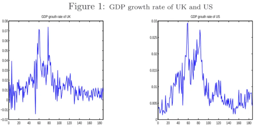
The empirical illustrations are based on gross domestic product (GDP) growth rate series of two countries: the United-States (US) and the United Kingdom (UK). GDP growth rate is calculated by the first difference of the logarithm of the quarterly GDP, as follows:
Xt= ∆(log(GDPt)) = log(
GDPt
GDPt−1). (25)
The data are sampled over the period from 1960Q1 to 2006Q4 and obtained from
International Financial Statistics data statistics, published by the IMF (GDP deflator
(2000=100)). In this section on synchronisation nonlinearity, GDP is used as a measure of economic activity. We restrict our analysis to bilateral links in order to avoid multi-collinearity between series. Note that for the evolutionary spectral estimation necessity, we lose ten observations at the beginning and ten at the end. Therefore we apply a different test to T − 20 (yielding 167 observations)1.
To respect the (j) and (jj) conditions we choose {ti} and {wj} as follows:
{ti = 18 + 20i}Ii=1 where I = [
T
20] and T the sample size, (26) [x] denotes the integer part of x.
{wj = 20π (1 + 3(j − 1))}7j=1 (27) To respect the (jj) condition, we inspect instability in these frequencies: π/20, 4π/20, 7π/20, 10π/20, 13π/20, 16π/20 and 19π/20.
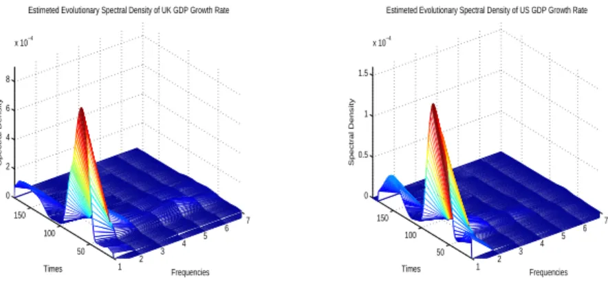
From the evolutionary spectral figure (2) we can conclude the change in importance of the low frequency cycles for the US and UK economies. This result is in line with that of Hughes Hallett and Richter (2006). The evolutionary spectrum seems to have similar forms but the importance of the low frequencies component in the UK is higher than that of the US. The two economies react approximately in the same way at the same time to the shocks but to different degrees. Compared with the time-varying coherence series, the dynamic cross-spectrum series is more stable at all frequencies. This is caused by the change in each evolutionary spectrum series.
4.2 Spectral and Cross-spectra Density Stability Test
The test of the structural changes of the spectral density amongst other things makes it possible to collect the instability of the coherence function. By using the wavelets and the theory of the local stationary process, Sachs et al. (2000) proposed a test which examines the stationarity of the auto-covariance function. Ahamada & Boutahar (2002) studied the stability of the spectral density around each time and each frequency by using the test of Tw. We follow them and we propose a nonparametric test for the stationarity of covariance based on the stability of the evolutionary spectral density. We extend their work to a sequential test of the stability in evolutionary cross-spectrum density.
4.2.1 Presentation of the Tests CSw
From the Cusum Test approach, we test the stability of the evolutionary cross-spectrum, by adopting the same strategy as Ahamada & Boutahar (2002) used in their test of the stability in evolutionary spectral density. For each of the two series of data {Xt}T
t=1 and
{Yt}Tt=1we can associate a time frequency cross-spectrum density SXY(w, t). Let {ti}Ii=1a set of size I representing a timescale in which all element respect the condition (j) of (7).
SXYiw = log(|SXY(w, ti)|) = log(AXY(w, ti)) = log([CXY2 (w, ti) + Q2XY(w, ti)]1/2). (28) Let Λiw XY = log(|SXY\(w, ti)|), µw = 1I PI i=1ΛiwXY, ˆσw2 = 1I PI i=1(ΛiwXY − µw)2 and δrw = 1 ˆ σw √ I r P i=1 (Λiw
XY − µw) when r = 1, ..., I. According to Priestley (1988), we have:
ΛiwXY ≈ SXYiw + eiwXY, (29)
where the sequence {eiwXY} is approximately normal, uncorrelated and identically
dis-tributed. We apply the Cusum test to the constancy of the evolutionary cross-spectrum density SXY(w, t).
Theorem 1. Let CSw = maxr=1,...,I|δrw|. Then, under the null hypothesis of stationarity
of Xt and Yt, the limiting distribution of CSw is given by: F1(a) = 1 − 2
∞ X k=1
(−1)k+1exp(−2k2a2), (30)
through the statistic of Kolmogorov-Smirnov we calculate the critical value Cα, ie.
P r(CSw > Cα) = α.2
4.2.2 Procedure for Detecting Breakpoints in Evolutionary Cross-Spectra For each w we calculate the statistic CSw and we reject the stability of cross-spectral density at level α if CSw > Cα. Therefore, when this statistic reaches its maximum in
rmax, this point is considered as a potential structural change date. We split the sample into two subsamples, and we do the same work in each of them. If CSw < Cα in the sub-period we accept the stability of the density function in w. In each subsample i, ri,max is an estimator of breakpoint if the null hypothesis of stability is rejected. We can therefore detect more than one break date for each frequency w. The test presented above has two main advantages in detecting structural change in both time and frequency. It detects endogenously structural change dates and reports the occurrence of the dates of break.
4.3 Time-Varying Coherence Function Stability Test (Bai & Perron,
1998-2001)
Some techniques have recently been developed to test multiple structural breaks. We adopt Bai & Perron’s (1998, 2001) test to detect a mean-shift in TVCF. Using GAUSS software, we obtain estimates by running the code created by Bai & Perron (1998, 2001). The choice of this type of model is motivated by TVCF characteristics. The graphical pattern of this statistic seems to be affected only by breaks in mean. Employing Bai & Perron’s test (1998) allows us to determine endogenously break dates when the change in coherence between series is significant. In this part, we are interested in breakpoint in the coherence between two economies. We define breakpoint as a change in the underlying relationship of the two economies that occurs as a response to an exogenous event or a change in monetary policy. 4.3.1 The Model and Estimators
We consider the following mean-shift model with m breaks, (T1, ..., Tm):
2C
T CV Fwj,t = µ1+ ut, t = 1, ..., T1,
T CV Fwj,t = µ2+ ut, t = T1+ 1, ..., T2,
.. .
T CV Fwj,t = µm+1+ ut, t = Tm+ 1, ..., T, (31)
for i = 1, 2, ..., m + 1, T0 = 0 and Tm+1 = T , where T is the sample size. T CV Fwj,t
is the time-varying coherence function in the neighborhood of the wj frequency. µi are the means, and utis the disturbance at time t. The breakpoints (T1, ..., Tm) are explicitly treated as unknown. From the ordinary least-squares (OLS) principle Bai & Perron (1998) estimate the vector of the regressor coefficients µj (1 ≤ j ≤ m + 1) by minimising the sum of squared residualsPm+1i=1 PTi
t=Ti−1+1(T CV Fwj,t− µi)2. Let \T CV Fwj,t({Tj}) denote the
resulting estimate. Substituting it in the objective function and denoting the resulting sum of squared residuals as ST(T1, . . . , Tm), we see that the estimated break dates
³ ˆ
T1, . . . , ˆTm ´ are such that
³ ˆ T1, . . . , ˆTm ´ = arg min (T1,...,Tm) ST(T1, . . . , Tm) , (32) where the minimisation is taken over all partitions (T1, . . . , Tm) such that Ti− Ti−1≥ [εT ].3
4.3.2 The Test Statistic and the Model Selection Criteria
This test locates multiple breaks without imposing any prior expectations on the data. The procedure estimates unknown regression coefficients together with the breakpoints when
T quarters are available. In order to determine the number of breakpoints, we use the
Bayesian Information Criterion (BIC) as suggested by Yao (1988) and defined as follows:
BIC(m) = (T−1ST( bT1, ..., bTm)) + p∗T−1ln(T ), (33) where p∗ = (m + 1)q + m is the number of unknown parameters. The author shows that, for normal sequence of random variables with shifts in mean, the number of breaks can be consistently estimated.
Bai & Perron (1998) present some asymptotic critical values for the arbitrary small positive number (ε) and the maximum possible number of breaks (M ): (ε = 0.10, M = 8), (ε = 0.15, M = 5), (ε = 0.20, M = 3) and (ε = 0.25, M = 2). For our empirical computation, we choose (ε = 0.15, M = 5) and we use Bai & Perron’s (1998, 2001) algorithm to obtain global minimisers of the squared residuals.
5
Empirical Illustration
’Many observers have noted how the shape of economic cycles has varied over time in terms of amplitude, duration and slope: long expansions, short recessions; expanding cycle lengths; steeper expansions than recessions and so on’(Hughes Hallett & Richter, 2006). To capture these features we use an evolutionary spectral approach and we propose a TVCF statistic based on this approach to detect the dynamic relationship between economies. Our study accommodates the possibility of structural breaks in these relationship caused by external events or a change in monetary policy. It also allows us to decompose movements into their component cycles and allow those cycles to vary in importance and characteristics over time. The aim of this study is to find whether the UK business cycle has changed in the
3[εT ] is interpreted as the minimal number of observations in each segment, where ε is an arbitrary
same way, to become more like the US one, or not. In time domain, the observed cyclical behaviour of the real business cycle hides many economic influences on cycles of different lengths and amplitudes. The use of frequency domain allows us to distinguish between properties of each cycle and to detect the dynamic coherence in each cycle. Because the spectral approach is nonparametric with no explicit economic structure imposed, we have many possibilities to explain the spectral peak. We will exemplify break dates detected in the first three frequencies, which correspond to the long-run effect. These frequencies also have an economic basis in business cycle literature: 20π, 4π20 and 7π20; correspond to 40 quarters’ (the Juglar fixed investment cycle (7-11 years)), ten quarters’ (the Kitchin inventory cycle (3-5 years)) and five quarters’ cycle length respectively.
Indeed, as regards international change in the nature and the amplitude of the distur-bance in world economy, we can find other fundamental factors that contribute to model cycles in the past and should continue to play a role, especially monetary and budgetary policies, globalisation, common shocks, actions executed by policymakers, etc.
We summarise in Tables (1 and 2) the results of the dynamic in comovement between the US and UK economies by looking for the tendency in level of synchronisation. We also find a clear difference in the comovement for the long term and the short term. Significant de-synchronisation in the two cycles (40 quarters, ten quarters) is observed between the two last regimes in contrast with the other cycle where we have an appreciation and a high level of synchronisation.
(1960Q1 − 1969Q2) During the Vietnam War in the late 1960s and early 1970s, the Johnson administration still applied the Keynesian policies adopted by that of Kennedy. The two factors seriously worsened the balance of payments. The sentiment of ’mini-recession’ in the US economy drives the de-synchronisation process, keeping a decrease in coherence for 0.474543 to 0.255965. Indeed, Artis et al. (1997) argue that an industrial production recession occurred in the UK around 1971.
(1980Q4, 1982Q1, 1984Q4 and 1987Q1): our argument in favour of these dates is the beginning of the globalisation period. A possible explanation for the latter dates is that, while the US liberalised its capital accounts in the 1970s, the UK did not remove all of the barriers on capital account transactions until the beginning of the 1980s. These dates concern an instability in the long, middle and short term because they appear in all frequencies. Loosely speaking, the effect of the financial integration was felt early on during the common shock period in the two countries, where the full impact of financial reforms occurred only during the globalisation period. Indeed, the federal reserve bank shifted to a less expansionary policy and adopted a new monetary policy based on inflation control and emphasised by interest rates. Inflation and unemployment decreased from 5.57% to 3.03% and from 7.27 to 5.67 respectively between the 1980s and the 1990s, in contrast with the average annual growth rate in real GDP, which stagnated at 3.02%. Curtis (2005) shows that federal reaction to variations in inflation rates and unemployment started in 1987Q1, and he concludes that the Fed’s objective was some mix of inflation-rate stability and output stability. It also corresponds to the Carter-Reagan defence build-up of the 1980s. Indeed, in the 1980s, the UK governments enacted a series of economic reforms to establish a more market-oriented economy. In sharp contrast with the convergence of inequality between the UK and the United States, the rates of poverty measured in absolute terms diverged between the two countries.
1991Q3, 1992Q2 and 1993Q2: we can explain these dates by the first Gulf War in the early 1990s and essentially the European Monetary System Crisis between 1992 and 1993. These dates are characterised by a general desynchronisation in the business cycles in all the OCDE countries. The crisis of the European exchange-rate mechanism (ERM) (1992 − 1993) was a critical event in the post-Bretton Woods history of the international monetary system. This event represents a turning-point in the use of exchange rate tools in the design of disinflation policies. The integration of two national economies under very different systems and with a substantial gap in productivity resulted in the adoption of
a controversial monetary-fiscal policy (Buiter, Corsetti & Pesenti, 1998). Increase in the German interest rate and in their public deficit adding to the speculative attack against the lira and later against the franc intensified the conflict on exchange-rate matters among European policymakers. ’Black Wednesday’ in the UK announced the beginning of the end of this exchange rate arrangement. On the morning of 16 September 1992, the Bank of England raised the minimum lending rate from 10% to 12%. On the same day, it announced a new increase to 15% and the ’temporary’ withdrawal of the pound from the ERM was announced. Later, Italy followed Britain out of the ERM. At the same time several European countries were the victims of speculative attacks against their money. The 1992-1993 ERM crisis created a macroeconomic disturbance not only in Europe but in the rest of the world.
1996Q3, 1998Q1: the UK economy continued to experience lower rates of productivity than its major competitors. In December 1998, the Government published a white paper outlining a variety of measures aimed at shifting the economy into a new era of success, based upon the idea of a ’knowledge-driven economy’. Britain had a productivity gap of 40% with the USA and 20% with France and Germany. In contrast with these differences in productivity common international shocks promoted synchronisation between the two economies. These dates correspond to a number of international events that seriously affected world economy: the East-Asian crisis in July 1997, the Russian cold (1998) and the Brazilian fever (1998). Through the spectral properties, we can say that these observed regime shifts concern the middle term.
Now we are interested in break dates at the short term: 1971Q1, 1975Q4, 1977Q2. We think that these dates summarise the persistence of relatively high inflation between the sixties and the seventies since annual inflation went up gradually from 2% to approximately 10% at the end of the seventies. In the United States, as in Great Britain, this increasing inflation rhythm started to accelerate a long time before the explosion of the import prices. The early/mid-1970s were also crisis years in the UK, with accelerating inflation, rising unemployment, massive industrial unrest and the first oil price shock (Dow, 1998).
6
Conclusion
In this paper, we propose a measure of comovement that is able to detect not only periods of convergence or divergence but to locate them endogenously and in different frequency. These findings allow us to distinguish between the properties of the cycles in the long term and the short term. We show, by applying these methods to GDP growth rate, how economic business cycles change over time and how synchronisation between US and UK business cycles changed from 1960 to 2006. As expected, the degree of synchronisation between the US and the UK has changed over time in all cycles, and the breakpoint in coherence series corresponds to the change in monetary policy, especially to that of the US. Our new methodology detects appropriately the known recessions of the mid-1970s, the beginning of the 1980s and 1992 to 1993. We also infer a higher degree of business synchronisation between US and UK economies, especially in short cycles. After 1992, we observe a divergence in the long-run cycles caused by a change in UK monetary policy.
Appendices
A
Proof of theorem 1.
Under the null assumption of the stability of the frequency w, the evolutionary spectral density is independent of time, i.e., SXiw = SX and SYiw = SY; of Piestley’s relation (8), we
have:
ΛiwX ≈ SXiw+ eiwX,
ΛiwY ≈ SYiw+ eiwY , i = 1, ..., I = [T
20].
We can suggest for this case a time-varying cross-spectrum which is independent of time, i.e., SXYiw = SXY; so we have:
ΛiwXY ≈ SXYiw + eiwXY, i = 1, ..., I = [T
20],
where the sequence eiwXY is approximately normal, uncorrelated and identically distributed. The estimator of SXY is given by ˆSXY = 1
I I P i=1
Λiw
XY = µj and the OLS residuals are c eiw = Λiw XY − µj. Thus δwr = σˆw1√I r P i=1
(ΛiwXY − µj) represents the cumulative sum of the OLS residuals. Let B(I)(z) = 1
ˆ σw √ I [Iz]P i=1 c
eiw for 0 ≤ z ≤ 1. Since all the conditions of the theorem of Ploberger & Krämer (1992) are trivially satisfied, then the limit in distribution of B(I)(z) is a Brownian bridge standard B(z). Therefore the limit in the distribution of
sup0≤z≤1|B(I)(z)| is sup0≤z≤1|B(z)|. According to Billingsley (1968), however, we have:
P (sup0≤z≤1|B(z)| > a) = 2
∞ X k=1
(−1)k+1exp(−2k2a2),
The desired conclusion holds, since CSt,w = maxr=1,...,I|δrw| = sup0≤z≤1|B(I)(z)|.
B
Figures
Figure 1: GDP growth rate of UK and US
0 20 40 60 80 100 120 140 160 180 −0.02 −0.01 0 0.01 0.02 0.03 0.04 0.05 0.06 0.07 0.08 GDP grouth rate of UK 0 20 40 60 80 100 120 140 160 180 0 0.005 0.01 0.015 0.02 0.025 0.03 GDP grouth rate of US
Figure 2: Evolutionary Spectrum of UK and US 1 2 3 4 5 6 7 50 100 150 0 2 4 6 8 x 10⁻⁴ Frequencies Estimeted Evolutionary Spectral Density of UK GDP Growth Rate
Times Spectral Density 1 2 3 4 5 6 7 50 100 150 0 0.5 1 1.5 x 10⁻⁴ Frequencies Estimeted Evolutionary Spectral Density of US GDP Growth Rate
Times
Spectral Density
Figure 3: Time Varying Cross-spectrum and Time Varying Coherence Function
1 2 3 4 5 6 7 50 100 150 0 1 2 3 4 5 x 10⁻⁵ Frequencies Estimeted Time Varying Cross Amplitude of US GDP Growth Rate and UK GDP Growth Rate
Times
Time varying cross amplitude
1 2 3 4 5 6 7 50 100 150 0 0.2 0.4 0.6 0.8 Frequencies Estimeted Time Varying Coherence Function of US GDP Growth Rateand UK GDP Growth Rate
Times
Time Varying Coherence Function
C
Tables
Table 1: Break Date Identification for the Evolutionary Cross-Spectrum of US and UK estimators Frequencies Tb1 Tb2 π/20 1982Q1 4π/20 1982Q1 7π/20 1982Q1 10π/20 1982Q1 1991Q3 13π/20 1982Q1 1996Q3 16π/20 1982Q1 19π/20 1982Q1
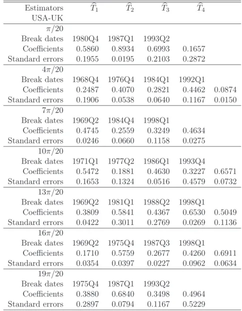
Table 2: Break Date Identification for the TVCF of US and UK at Different Frequency Estimators Tb1 Tb2 Tb3 Tb4 USA-UK π/20 Break dates 1980Q4 1987Q1 1993Q2 Coefficients 0.5860 0.8934 0.6993 0.1657 Standard errors 0.1955 0.0195 0.2103 0.2872 4π/20 Break dates 1968Q4 1976Q4 1984Q1 1992Q1 Coefficients 0.2487 0.4070 0.2821 0.4462 0.0874 Standard errors 0.1906 0.0538 0.0640 0.1167 0.0150 7π/20 Break dates 1969Q2 1984Q4 1998Q1 Coefficients 0.4745 0.2559 0.3249 0.4634 Standard errors 0.0246 0.0660 0.1158 0.0275 10π/20 Break dates 1971Q1 1977Q2 1986Q1 1993Q4 Coefficients 0.5472 0.1881 0.4630 0.3227 0.6571 Standard errors 0.1653 0.1324 0.0516 0.4579 0.0732 13π/20 Break dates 1969Q2 1981Q1 1988Q2 1998Q1 Coefficients 0.3809 0.5841 0.4367 0.6530 0.5049 Standard errors 0.0422 0.3011 0.2769 0.0269 0.1136 16π/20 Break dates 1969Q2 1975Q4 1987Q3 1998Q1 Coefficients 0.1710 0.5759 0.2677 0.4260 0.6911 Standard errors 0.0354 0.0397 0.0227 0.0962 0.0634 19π/20 Break dates 1975Q4 1987Q1 1993Q2 Coefficients 0.3880 0.6840 0.3498 0.4964 Standard errors 0.2897 0.0794 0.1167 0.5229
References
[1] Ahamada, I. & Ben Aïssa, M.S. (2003): Changements structurels dans la dynamique de l’inflation aux Etats-Unis : Approches non paramétriques. Annales d’Economie et de Statistique, n◦ 77, 2005.
[2] Ahamada, I. & Boutahar, M. (2002): Tests for covariance stationarity and white noise, with application to Euro/US Dollar exchange rate. Economics Letters 77, 177-186.
[3] Artis, M.J., Kontolemis, Z. & Osborn, D.R. (1997): Business Cycles for G7 and European Countries. Journal of Business 70, 249-279.
[4] Bai, J. & Perron, P. (1998): Estimating and testing linear models with multiple structural changes. Econometrica 66, 47-78.
[5] Bai, J. & Perron, P. (2001): Multiple structural change models: a simulation analysis, unpublished manuscript, Department of Economics, Boston University.
[6] Bai, J. & Perron, P. (2003a): Additional critical values for multiple structural changes tests. Econometrics Journal 6, 72-78.
[7] Bai, J. & Perron, P. (2003b): Computation and analysis of multiple structural change models. Journal of Applied Econometrics 18, 1-22.
[8] Ben Aïssa M.S., Boutahar M. & Jouini J. (2004): The Bai and Perron’s and Spec-tral Density Methods for Structural Change Detection in the U.S. Inflation Process. Applied Economics Letters 11 (2/10), 109-115.
[9] Ben Aïssa, M.S. & Jouini J. (2003): Structural Breaks in the U.S. Inflation Process. Applied Economics Letters 10 (10/15).
[10] Buiter, W., Corsetti, G. & Pesenti, P. (1998): Interpreting the ERM Crisis: Country-Specific and Systemic Issues. Princeton Studies in International Economics 84, Inter-national Economics Section, Department of Economics Princeton University.
[11] Chauvet, M., & Potter, S. (2001): Recent Changes in the US Business Cycle: mimeo, University of California.
[12] Croux, C., Forni, M. & Reichlin, L. (2001): A measure of comovement for economic variables: Theory and Empirics. The Review of Economics and Statistics, 83(2), 232-241.
[13] Curtis, D. (2005): Monetary Policy and Economic Activity in Canada in the 1990s. Canadian Public Policy / Analyse de Politiques, 31 (1), 59-77.
[14] Dow, C. (1998): Major recessions: Britain and the world, 1920-1995. Oxford: Oxford University Press.
[15] Duarte, A. & Holden, K. (2003): The business cycle in the G-7 economies. Interna-tional Journal of Forecasting 19, 685-700.
[16] Essaadi, E., Jouini, J. & Khallouli, W. (2007): The Asian Crisis Contagion: A Dy-namic Correlation Approach Analysis. GATE Working Paper No. 07-25.
[17] Hughes Hallett, A. & Richter, C. (2002): Are capital markets efficient? Evidence from the term structure of interest rates in Europe. The Economic and Social Review, 33 (3), 333-356.
[18] Hughes Hallett, A. & Richter, C. (2004): Spectral analysis as a tool for financial policy: An analysis of the Short-End of the British term structure. Computational Economics, 23, 271-288.
[19] Hughes Hallett, A. & Richter, C. (2006): Measuring the degree of convergence among European business cycles. Computational Economics, 27, 229-259.
[20] Hughes Hallett, A. & Richter, C. (2008): Have the Eurozone economies converged on a common European cycle?. International Economics and Economic Policy, 5 (1-2), 71-101.
[21] Jouini, J. & Boutahar, M. (2003): Structural breaks in the U.S. inflation process: a further investigation. Applied Economics Letters, 10 (15/15), 985-988.
[22] Loynes, R. M. (1968) : On the concept of the spectrum for non-stationary processes. J. Roy. Statist. Soc., Ser. B, 30, 1-20.
[23] McCullough, B. D. (1995): A spectral analysis of transactions stock market data. The Financial Review, 30 (4), 823-842.
[24] Pagan, A. & Schwert, W. (1990): Alternative models for conditional stock volatility. Journal of Econometrics 45, 267-290.
[25] Picard, D. (1985): Testing and Estimating Change-Points in Time Series. Adv. Appl. Probab. 17, 841-285.
[26] Ploberger, W. and Kramer, W. (1992): The Cusum Test with OLS Residuals. Ecoc-nometrica, 60 (2), 271-285.
[27] Priestley, M.B. & Chao, M.T. (1972): Non-Parametric Function Fitting. Journal of the Royal Statistical Society. Series B (Methodological), 34 (3), 385-392.
[28] Priestley, M.B. & Subba Rao, T. (1968): A Test for Non-stationrity of Time-series. University of Manchester, Institute of Science and Technology.
[29] Priestley, M.B. (1965): The Role of Bandwidth in Spectral Analysis. Applied Statis-tics, 14 (1), 33-47.
[30] Priestley, M.B. (1965): Evolutionary Spectra and Non-Stationary Processes. Journal of the Royal Statistical Society. Series B (Methodological), 27 (2), 204-237.
[31] Priestley, M.B. (1966): Design Relations for Non-Stationary Processes. Journal of the Royal Statistical Society. Series B (Methodological), 28 (1), 228-240.
[32] Priestley, M.B. (1978): Non-Linear Models in Time Series Analysis. The Statistician, 27 (34), 159-176.
[33] Priestley, M.B. (1988): Non-linear and non-stationary time series analysis. Academic Press: London.
[34] Priestley, M.B. (1996): Wavelets and Time-Dependent Spectral Analysis. J. Time Ser. Anal., 17 (1).
[35] Von Sachs, R. & Neumann, M., H. (2000): A wavelet-Based Test for Stationary. J. Time Ser. Anal., 21 (5).
[36] Yao, Y-C. (1988): Estimating the number of change-points via Schwarz’ criterion. Statistics and Probability Letters, 6, 181-189.
[37] Zhao, H., Lu, S., Zou, R., Ju, K. & Chon, K.H. (2005): Estimation of Time-Varying Coherence Function Using Time-Varying Transfer Functions. Annals of Biomedical Engineering, 33 (11), 1582-1594.