HAL Id: hal-01935261
https://hal.archives-ouvertes.fr/hal-01935261
Submitted on 26 Nov 2018
HAL is a multi-disciplinary open access
archive for the deposit and dissemination of
sci-entific research documents, whether they are
pub-lished or not. The documents may come from
teaching and research institutions in France or
abroad, or from public or private research centers.
L’archive ouverte pluridisciplinaire HAL, est
destinée au dépôt et à la diffusion de documents
scientifiques de niveau recherche, publiés ou non,
émanant des établissements d’enseignement et de
recherche français ou étrangers, des laboratoires
publics ou privés.
ELEPHANT” PHENOMENON AND ITS
NUMERICAL VISUALIZATION
Roberta Bianchini, Laurent Gosse, Enrique Zuazua
To cite this version:
Roberta Bianchini, Laurent Gosse, Enrique Zuazua. A TWO-DIMENSIONAL ”FLEA ON THE
ELEPHANT” PHENOMENON AND ITS NUMERICAL VISUALIZATION. Multiscale Modeling
and Simulation: A SIAM Interdisciplinary Journal, Society for Industrial and Applied Mathematics,
2019, 17 (1), pp.137-166. �hal-01935261�
PHENOMENON AND ITS NUMERICAL VISUALIZATION ROBERTA BIANCHINI∗, LAURENT GOSSE†, AND ENRIQUE ZUAZUA‡
Abstract. Localization phenomena (sometimes called “flea on the elephant”) for the operator
Lε=−ε2∆u + p(x)u, p(x) being an asymmetric double-well potential, are studied both analytically
and numerically, mostly in two space dimensions within a perturbative framework. Starting from a classical harmonic potential, the effects of various perturbations are retrieved, especially in the case of two asymmetric potential wells. These findings are illustrated numerically by means of an original algorithm, which relies on a discrete approximation of the Steklov-Poincaré operator for Lε,
and for which error estimates are established. Such a two-dimensional discretization produces less mesh-imprinting than more standard finite-differences and captures correctly sharp layers.
Key words. Asymmetric double-well potential; Lipschitz domains; Schrödinger equation; AMS subject classifications. 35P20, 35Q40, 65N06, 65N15.
1. Introduction and preliminaries. The “flea on the elephant” is an
expres-sion coined by Barry Simon in [47] to describe the following counter-intuitive phe-nomenon: being V (x, y) a symmetric (smooth) two-well potential and V + δV an arbitrarily small (smooth) perturbation of it, then for 0 < ε ≪ 1, corresponding
perturbed eigenfunctions will preferably localize in the largest well (see also [38]).
1.1. Elementary ”flea on the elephant” in 1D. Given ε > 0, we start from
the steady one-dimensional Schrödinger equation for some energy level Eε,
−ε∂xxψε+ V (x)ψε= Eεψε(x), x∈ (0, 1),
where, for 0 < a < b < 1, the (square-wells) potential V (x) is piecewise constant,
V (x) = ¯V χx∈(a,b)+∞
(
χx<0+ χx>1
)
, V > 0.¯
Dirichlet conditions correspond to infinite potential walls: ψ(0) = ψ(1) = 0,
k := k(Eε) = √ Eε ε , κ := κ(Eε) = √ ¯ V − Eε ε ,
describe bound-states, so that,
∀x ∈ (0, 1), ψ(x) =
A sin kx, x∈ (0, a)
B exp(κ(x− a)) + C exp(κ(b − x)),
D sin k(1− x), x∈ (b, 1),
where (real) constants A, B, C, D are such that C1smoothness holds:
A sin ka = B + C exp(κ(b− a)) D sin k(1− b) = B exp(κ(b − a)) + C
}
C0 smoothness,
kA cos ka = κ[B− C exp(κ(b − a))] −kD cos k(1 − b) = κ[B exp(κ(b − a)) − C]
}
C1 smoothness,
(1.1)
∗Unité de mathématiques pures et appliquées, École normale supérieure de Lyon, 46, allée d’Italie
69364 Lyon Cedex 07 (France). [email protected]
†IAC–CNR “Mauro Picone”, Via dei Taurini 19, 00185 Rome (Italy) [email protected] ‡DeustoTech, University of Deusto, 48007 Bilbao, Basque Country (Spain),
Depar-tamento de Matemáticas, Universidad Autónoma de Madrid, 28049 Madrid, (Spain). [email protected]
The vector of coefficients can be characterized by means of the kernel of a 4×4 matrix,
sin ka −1 − exp(κ(b − a)) 0
0 − exp(κ(b − a)) −1 sin k(1− b)
k
κcos ka −1 exp(κ(b− a)) 0
0 exp(κ(b− a)) −1 kκcos k(1− b) = 0. Since (1.1) implies,
A(κ sin ka + k cos ka)
D(κ sin k(1− b) − k cos k(1 − b))= exp(κ(a− b)), A(κ sin ka− k cos ka)
D(κ sin k(1− b) + k cos k(1 − b))= exp(κ(b− a)),
then
A2cos2ka(κ2tan2ka− k2)
D2cos2k(1− b)(κ2tan2k(1− b) − k2) = 1, (1.2)
so that, when a = 1− b in (1.2), symmetry, D2= A2, easily follows. The asymmetric
case is less straightforward in terms of algebra, even in 1D, see for instance [20, 31, 38, 45, 49] and [26, Chapter 2]. Accordingly, numerical simulations of a 1D explicit example are displayed in Fig. 1.1. Finite-differences based onL-splines and borrowed
Figure 1.1. Eigenfunctions for symmetric (left) vs. asymmetric (right) square wells.
from [18] were set up in order to maximize both stability and accuracy in this context of a square-well potential: namely, we implemented both,
a = 0.35, b = 0.65 on the left, a = 0.35, b = 0.675 on the right,
with ε = 0.001, 27grid points, and the following discretization,
rj±1 2 = √ V (xj±1 2) ε , − ε ∆x [ rj+1 2 sinh(rj+1 2∆x) ( ψj+1− cosh(rj+1 2∆x)ψj ) − rj−1 2 sinh(rj−1 2∆x) ( cosh(rj−1 2∆x)ψj− ψj−1 )] = Eεψj.
The (Anderson-like) localization process [14] is easy to see; similar behavior occurs in 2D, too, as shown in Fig. 5.5 for two symmetric, and asymmetric, Gaussian well po-tentials. Heuristically, it is explained by recalling that the curvature of eigenfunctions grows with their energy: the widest well (lying at the same depth) allows the ground state to have a larger wavelength, hence a smaller curvature. This kind of strong Accumulation phenomenon due to any little perturbation is known in literature as “the flea on the elephant”, with a complete analysis given in [7, 32, 39, 44, 48].
1.2. Plan of the paper. In several dimensions, the spectral effects of perturbing
a quadratic potential were studied in the literature, see for instance [32, 27, 47, 48, 30]. In those papers, from both a mathematical physics and a functional analysis perspective, many results were stated; there are also other probabilistic approaches in this direction, with applications to large deviations, see [46] and more recent references quoted in [30]. Accordingly, in Section 2, basic results for the harmonic potential are derived, so that, in Section 3, perturbations can be studied, especially concerning the width of the wells and their location. Section 4 deals with a 2D extension of the “L-spline scheme” set up in 1D: its derivation follows [17] and is presented in §4.1
and some error estimates are given in §4.3. Section 5 contains some computational results, mostly for the accuracy on the harmonic potential in a square domain, and for perturbations of a two-well potential. Concluding remarks are given in Section 6, where the ability of the 2D scheme to capture sharp layers is illustrated in Fig. 6.1. Appendix A recalls regularity results for elliptic equations in square domains, following either [8, 21, 29] or [2, 28, 34, 24] for a study of “compatibility conditions”.
2. Gaussian eigenfunctions of the quadratic potential. Let a differential
operator Lε(u) :=−ε2∆u + p(x)u have a potential with conditions [P]:
• p(x) ∈ C2(RN), p(x)≥ 0;
• p(x) has exactly two quadratic minima located in xi, for i = 1, 2
lim x→xi
p(x) |x − xi|2
= Ci, for some constants Ci.
More general potentials were considered in, e.g., [7, 26, 39, 44]. In the whole space
x∈ RN, the eigenvalue problem for the harmonic oscillator reads,
p(x) = N 2 + |x|2 4ε2, L ε(u) =−ε2∆u + ( N 2 + |x|2 4ε2 ) u, (2.1)
being| · | the Euclidean norm. Inserting a change of variables, ∀x ∈ RN, u(x) := exp
(
|x|2
4ε2
)
w(x) inside Lε(u) = λu, (2.2) yields a (steady) convection-diffusion equation,
˜ Lε(w) := exp ( −|x|2 4ε2 ) Lε(u) =(− ε2∆w− x · ∇w)= λw. (2.3) Namely, in terms of the new variable w(x), the spectral problem (2.1) reads
Convection-diffusion problem (2.4) recasts as a drift-diffusion (conservative) one, − ε2∇ · (Kε (x)∇w) − λwKε(x) = 0, Kε(x) = exp ( |x|2 2ε2 ) , (2.5) so that nontrivial solutions to (2.4) are critical points of the following functional:
f 7→ Eε(f ) = ε2 2 ∫ RN |∇f|2Kε(x) dx−λ 2 ∫ RN |f(x)|2Kε(x) dx, (2.6)
for f belonging, for ε fixed, to the following “weighted Sobolev space”,
H1(Kε) = { f :RN → R : ∫ RN ( |f|2+ ε2|∇f|2)Kε(x) dx < +∞ } . (2.7)
Proposition 1. For Kε(x) being as in (2.5) and H1(Kε) given by (2.7), the
continuous embedding H1(Kε)⊂ L2(Kε) is compact,
H1(Kε)⊂⊂ L2(Kε) := { f :RN → R : ∫ RN |f|2Kε(x) dx < +∞ } .
Proof. The proof contained in [13] applies, based on the following lemma:
Lemma 1. For any f ∈ C1
c(RN), the Poincaré inequality holds:
∫ RN |f|2 ( N 2 + |x|2 4ε2 ) Kε(x) dx≤ ε2 ∫ RN |∇f|2Kε(x) dx. (2.8)
The differential operator ˜Lεin (2.3) is set in the domain
D( ˜Lε) = {
f ∈ H1(Kε); ˜Lεf ∈ L2(Kε) }
:= H2(Kε), (2.9) in which it is self-adjoint and, by Proposition 1, D( ˜Lε)⊂⊂ L2(Kε) compactly em-bedded. This implies that ˜Lε presents an increasing sequence of eigenvalues (λk)k≥0,
where λ0> 0 is guaranteed by inequality (2.8). Moreover, for any m≥ 0,
if f ∈ L2(Kε), then (1 +|ξ|2)m2fˆ∈ L2(RN),
so that the Fourier transform ˆf is smooth,
∀m ≥ 0, fˆ∈ Hm(RN), fˆ∈ C∞(RN).
It remains to take the Fourier transform of (2.4),
ε2|ξ|2w(ξ)+N ˆˆ w(ξ)+ξ·∇ ˆw(ξ) = λ ˆw(ξ), (x\j∂xjw)(ξ) =− ˆw(ξ)−ξj∂ξjw(ξ). (2.10)ˆ Another change of variables yields,
ξ· ∇v(ξ) = (λ − N)v(ξ), v(ξ) = exp(ε2|ξ|
2
2 ) ˆw(ξ),
thus, v(ξ) is a polynomial function of degree (λ− N) = k − 1, k ∈ N, namely v(ξ) = Pk−1(ξ), Pk−1(ξ) homogeneous polynomial of degree k− 1,
and solutions to (2.10) satisfy ˆw(ξ) = exp(−ε2|ξ|2/2)P
k−1(ξ), see also [13].
Theorem 2.1. The eigenvalues of ˜Lε in (2.3), where D( ˜Lε)⊂⊂ H1(Kε), are
λk = N + k− 1, k ∈ N, (2.11)
with the ground-state and its related eigenfunctions, ϕε0(x) := exp ( −|x|2 2ε2 ) , Dαϕε0(x), α = (α1,· · · , αN), |α| = k − 1.
3. Perturbation analysis of the two wells potential. Hereafter, double well
potentials with identical and different wells are considered, in order to show the role played by symmetry. In the symmetric case with ε≪ 1, eigenfunctions accumulate
equally in both wells; oppositely, for asymmetric potentials, the ground state fills mostly the widest well (see [30] for more of a differential geometry approach). We qualitatively analyze effects of symmetry breaking in the potential shape p(x):
• accumulation of solutions in the widest well; • the role played by the position of the perturbation;
• how a perturbation affects the spectrum of the original problem.
Consider the spectral problem associated with
D(Lε)∋ u 7→ Lε(u) =−ε2∆u +p(x)
4ε2 u, where p(x) satifies [P], (3.1)
the following statements hold true:
• the ground state accumulates in the widest well;
• potential perturbations’ affect the spectral problem as much as they are close
to the wells;
• eigenvalues and eigenfunctions’ modifications occur according to the way the
perturbation acts on the eigenfunctions of the original spectral problem.
3.1. Accumulation in the widest well. Yet, pick 0 < ε ≪ 1, and consider
the spectral problem (3.1), mostly when p(x) is a C2(RN) has two wells at the same
height but with possibly different widths. Its eigenvalues form an increasing sequence, whose minimum λ1is given by Rayleigh’s quotient,
λ1= inf u∈D(Lε) ∫ RNε 2|∇u|2+p(x) 4ε2|u| 2dx ∫ RN|u|2dx . (3.2)
Defining the measure dp = p(x) dx, Rayleigh’s quotient rewrites
λ1= inf u∈D(Lε) ∫ RNε 2|∇u|2dx + 1 4ε2 ∫ RN|u| 2dp ∫ RN|u|2dx .
Lemma 2. Let x0 be any point located at any positive and fixed distance from 0.
Let d > 0: the first eigenvalue ˜λ0 associated with the operator,
Lε=−ε2∆ + p(x) 4ε2 , p(x) =|x| 2χ BR(0)+ d|x − x0| 2χ BR(x0), (3.3)
satisfies, for a positive constant value c, the following expansion:
λ˜0− N 2 = O ( R2 ε2 ) exp ( −cR2 ε2 ) . (3.4)
The shift between eigenvalues (3.4) and (2.11) comes from the factor N
2 in (2.1).
Proof. The Rayleigh quotient reads:
˜ λ0= min ψ∈H1(R2) ∫ R2 ε2|∇ψ(x)|2+|ψ(x)| 2 4ε2 ( |x|2χ BR(0)+ d|x − x0| 2χ BR(x0) ) dx ∫ R2 |ψ(x)|2dx . (3.5)
From Section 2, ϕ0(x) = exp(−|x| 2 4ε2) solves −ε 2∆ϕ 0+|x| 2 4ε2ϕ0= N 2 ϕ0, where N 2 = λ0=ψ∈Hmin1(R2) ∫ R2 ε2|∇ψ(x)|2+|x| 2 4ε2|ψ(x)| 2dx ∫ R2|ψ(x)| 2dx = ∫ R2 ε2|∇ϕ0(x)|2+ |x|2 4ε2|ϕ0(x)| 2dx ∫ R2|ϕ 0(x)|2dx . (3.6)
The explicit expression of λ0, provided by the Rayleigh quotient, can be used in ˜λ0
in (3.5), in order to get the desired approximation. More precisely, by substituting
ϕ0(x) in the previous expression, the upper bound is given by
˜ λ0≤ N 2 + 1 2πε2 (∫ R2 |x|2exp(−|x|2 2ε2) 4ε2 (χBR(0)− 1) dx + ∫ R2 d|x − x0|2χBR(x0) exp(−|x|2ε22) 4ε2 dx ) .
On the other hand, the lower bound,
˜ λ0= min ψ∈H1(R2) ∫ R2 ε2|∇ψ(x)|2+|ψ(x)| 2 4ε2 ( |x|2χ BR(0)+ d|x − x0| 2χ BR(x0) ) dx ∫ R2|ψ(x)| 2dx = min ψ∈H1(R2) (∫ R2 ε2|∇ψ(x)|2+|x| 2 4ε2|ψ(x)| 2dx ∫ R2|ψ(x)| 2dx + ∫ R2|ψ(x)| 2|x|2 4ε2(χBR(0)− 1) dx ∫ R2|ψ(x)| 2dx + ∫ R2|ψ(x)| 2d|x − x0|2 4ε2 χBR(x0)dx ∫ R2|ψ(x)| 2dx )
≥ min ψ∈H1(R2) ∫ R2 ε2|∇ψ(x)|2+|x| 2 4ε2|ψ(x)| 2dx ∫ R2|ψ(x)| 2dx − (∫ R2| ˜ ψ(x)|2|x| 2 4ε2(χBR(0)− 1) dx ∫ R2| ˜ ψ(x)|2dx + ∫ R2| ˜ ψ(x)|2d|x − x0| 2 4ε2 χBR(x0)dx ∫ R2| ˜ ψ(x)|2dx ) ,
where the last inequality holds for ˜ψ(x) ∈ H1(R2), being all the addends in the previous line positive. By using again (3.6) and setting ˜ψ(x) = ϕ0(x), one gets
˜ λ0≥ N 2 − 1 2πε2 (∫ R2 |x|2exp(−|x|2 2ε2) 4ε2 (χBR(0)− 1) dx + ∫ R2 d|x − x0|2χBR(x0) exp(−|x|2ε22) 4ε2 dx ) .
Passing to polar coordinates, 1 2πε2 ∫ R2 |x|2 4ε2(Id− χBR(0))|ϕ0(x)| 2dx = 1 8πε4 ∫ 2π 0 dθ ∫ ∞ R ρ3 exp(−ρ 2 2ε2) dρ = (R2+ 2ε2) 4ε2 exp(− R2 2ε2), ∫ R2 exp(−|x| 2 2ε2) dx = 2πε 2.
Remark 1. Lemma 2 implies that λ0 = N2 is a good approximation for the
expression of the first eigenvalue when the potential only has two wells. Performing exactly the same computations with ϕd
0(x) = exp(−
d|x−x0|2
4ε2 ), one gets λ d
0 = N d2 .
However, in this case the error term in the expansion is bigger, meaning that this approximation is less accurate than the one provided by the widest Gaussian.
The parameter d > 0 in (3.3) controls the convexity of the well centered in x0. If
the potential p(x) has different wells, the ground state is known to accumulate only in one well, see [48, 27, 30]. From Lemma 2 (and Remark 1), the expression of the first eigenvalue ˜λ0= N2 + O ( R2 ε2 ) exp ( −cR2 ε2 )
is reached by ϕ0(x). This suggests
that the accumulation well should be the one provided by |x|4ε22.
Definition 1 (see [42, 43]). For a fixed ˜λ ∈ R, a quasi-eigenfunction is any function u(x)∈ D(Lε) such that the following “error function”,
Err(u) :=−ε2∆u +p(x) 4ε2 u− ˜λu,
satisfies, for any C(ε) exponentially decreasing, the inequality: ∥Err(u)∥L1(RN)≤ C(ε), ε≪ 1.
In the next Lemma, we show that ϕ0(x) is a quasi-eigenfunction of Lε in (3.3),
in the sense of Definition 1. Identical computations bring that
ϕd0(x) := exp (
−d|x − x0|2
4ε2
)
is a quasi-eigenfunction of the operator defined in (3.3), too. However, it turns out that ϕ0(x) is a better approximation of the ground-state of (3.3) than ϕd0(x). The
meaning of the last sentence is clarified below.
Lemma 3. Under the hypotheses of Lemma 2, let us fix d > 1. Then
∥Err(ϕ0)∥L1(RN)<∥Err(ϕd0)∥L1(RN), ϕd0(x) = exp(−
d|x − x0|2
4ε2 ). (3.7)
Proof. Thanks to Lemma 2, in terms of the Rayleigh quotient,
˜ λ0= N 2 + O ( R2 ε2 ) exp ( −cR2 ε2 ) ,
is reached by ϕ0(x). This way, by comparing the two problems,
−ε2 ∆ϕ0+ p(x) 4ε2 ϕ0= N 2ϕ0+ Err(ϕ0), −ε 2 ∆ϕd0+ p(x) 4ε2 ϕ d 0= N 2ϕ d 0+ Err(ϕ d 0), with p(x) in (3.3), where Err(ϕ0) = [ |x|2 4ε2(χBR(0)− Id) + d|x − x0|2 4ε2 χBR(x0) ] ϕ0, Err(ϕd0) = [ d|x − x0|2 4ε2 (χBR(x0)− Id) + |x|2 4ε2χBR(0)+ N (d− 1) 2 ] ϕd0,
and integrating in space, one gets (3.7). After proving that
• the best approximation for the first eigenvalue associated with Lε in (3.3),
˜
λ0≈N2, is provided by ϕ0(x) (Lemma 2),
• ϕ0(x) is the best quasi-eigenfunction (Lemma 3),
we finally show that the solution to the spectral problem accumulates in |x|4ε22, the
widest well.
Proposition 2. Le p(x) be a double well potential satisfying conditions [P].
Let x1, x2 be the centers of the two potential wells, and x1 be the widest one. The
(normalized) solution u(x) ∈ H1(Kε) to the spectral problem associated with (3.3)
accumulates in the widest well. More precisely, for a fixed ε > 0, let BR(xi) be the
disk of radius R > 0 and center xi, i = 1, 2, there exists ε0> 0 such that,
∀ε ≤ ε0, ∫ BR(x1) |u(x)|2dp > exp ( c|x1− x2|2 ε2 ) ∫ BR(x2) |u(x)|2dp.
Proof. Without loss of generality, we consider Lεin (3.3). The first eigenfunction
is well approximated by ϕ0(x). This way,
∫ BR(0) |ϕ0(x)|2dp = ∫ BR(0) |ϕ0(x)|2|x| 2 4ε2 dx = 2π ∫ R 0 exp(−ρ 2 2ε2) ρ 3dρ; ∫ BR(x0) |ϕ0(x)|2dp = ∫ BR(x0) |ϕ0(x)|2 d|x − x0|2 2ε2 dx = d exp(−|x0| 2 2ε2 ) ∫ 2π 0 dθ ∫ R 0 exp(−ρ 2− 2ρx
0cos θ− 2ρy0sin θ
2ε2 ) ρ 3dρ ≥ 2πd exp(−|x0|2 ε2 ) ∫ R 0 exp(−ρ 2 ε2) ρ 3dρ,
which ends the proof.
3.2. Distance from the wells. Given a potential well and a localized
pertur-bation: does the distance between each other affect the spectral problem ? If wells are far enough from each other, this is a local question which is addressed by perturbing the harmonic potential. Hereafter, ε = 1 and the term N
2 in (2.1) is ignored, L(u) =−∆u +|x| 2 4 u, ϕ0(x) = exp(− |x|2 4 ). (3.8)
Let a small perturbation be given by χBR(x0)(x), the characteristic function of a disk
centered in x0 of radius R > 0, and consider a perturbed spectral problem,
LR(u) =−∆u +|x|
2
4 u + χBR(x0)u = λu. (3.9)
The ground-state ϕ0(x) of (3.8) can be seen as an quasi-eigenfunction for the
per-turbed problem (3.9), as it almost satisfies the spectral equation for LR(u),
−∆ϕ0+ |x|2 4 ϕ0+ χBR(x0)ϕ0≈ λϕ0, with an error Err(x0) = χBR(x0)ϕ0(x) = χBR(x0)exp(− |x|2 4 ).
In one dimension, N = 1, such an error is easy to quantify, for instance in L1,
x07→ ∥Err(x0)∥L1(R)= ∫ x0+R x0−R exp(−|x| 2 4 ) dx. so that its variations with respect to x0∈ R satisfy:
d dx0 ∥Err(x0)∥L1(R)= exp(− x0+ R 2 2)− exp(− x0− R 2 2) = { < 0, (x0> 0), > 0, (x0< 0).
This derivative shows that,
• the position x0= 0 is a local maximum for∥Err(x0)∥L1(R);
• the perturbation’s effects on (3.8) decrease with both |x0| and R.
This elementary argument can be extended to N dimensions; precise results on the role of the position of the perturbation are given in, e.g. [48].
3.3. Variations of the spectral components. Coming back to a general
po-tential p(x) in (3.1), we consider L(u) in (3.8), where λ, u are any eigenvalue and normalized eigenfunction. Let M be any linear bounded operator and δ≪ 1 a
con-stant small enough: again, we treat λ as a quasi-eigenvalue for the perturbed operator,
Lu + δM u = λu + Errδ(u), where Errδ(u) = δM u. (3.10) We take the derivative of (3.10) w.r.t. δ, calculated in δ = 0,
Lu′+ M u = λ′u + λu′+ O(∥Mu∥), where ·′:= d
dδ
δ=0
Namely,
(L− λ)u′= (λ′− M)u + O(∥Mu∥). (3.11) Since λ is an eigenvalue of L, associated with the eigenfunction u, then u∈ Ker(L−λ).
Fredholm’s Alternative implies that there exist solutions u′ to (3.11) such that (λ′− M)u + O(∥Mu∥) ⊥ Ker(L − λ),
i.e., denoting by <·, · > the L2 scalar product,
< (λ′− M)u, u >= O(∥Mu∥), ∥u∥2=< u, u >= 1, then, λ′ = d dδ δ=0 λ(δ) =< M u, u > +O(∥Mu∥), (3.12) namely
|λ′| ≤ ∥Mu∥∥u∥ + O(∥Mu∥) = ∥Mu∥ + O(∥Mu∥),
so that the perturbation δM affects eigenvalues according to the way M affects the original eigenfunction u. Yet, we look at the variations of this eigenfunction by taking the derivative with respect to δ of the scalar product∥u∥2=< u, u >= 1.
1 2 d dδ δ=0 (∥u∥2) =< u, u′>= 0, i.e. u′⊥ u.
Orthogonality u′⊥ u and (L − λ)u′⊥ u, along with Fredholm’s Alternative imply
u′ is proportional to (λ′− M)u + O(∥Mu∥) = (L − λ)u′,
so that, locally for δ≃ 0,
∥u′∥ ≤ C∥Mu∥ for a given constant value C(λ).
4. Two-dimensional “Steklov numerical scheme”. In this section, a
deriva-tion is recalled from [17], in order to establish several properties in close reladeriva-tion with the original problem of the “flea on the elephant”. Hereafter, we shall always work on a uniform, Cartesian computational grid, with ∆x = ∆y.
b b b b b
u
ni,ju
ni+1,ju
ni,j+1u
ni,j−1u
ni−1,j⊗
⊗
⊗
⊗
¯
α
i−1 2,j− 1 2Figure 4.1. Transmission conditions at un
i,j given by Steklov-Poincaré operators.
4.1. Derivation of the numerical process. Consider the stationary, strictly
elliptic and coercive, two-dimensional problem, {
−∆u + α2(x, y)u = 0, (x, y)∈ Ω,
u(x, y) = g(x), (x, y)∈ ∂Ω, (4.1) where Ω is a polygonal domain of R2. The numerical simulations, carried out with
the “Steklov scheme” [17], and presented below mostly focus on the spectral analysis associated with the strictly elliptic operator L(u) :=−∆u + α2(x, y)u. Accordingly,
we shall work on the square (Lipschtiz) domain Ω = (0, 1)2⊂ R2, so that the typical
regularity for u should be at least H2(Ω), see [8, 21]. We refer to Appendix A for
elementary regularity results for problems like (4.1) in a square domain: in particular, when the compatibility conditions (A.2) hold at each corner, the Hölder regularity of inhomogeneous Dirichlet data g passes to the solution u, see Theorem A.2.
The “Steklov scheme”, see [17, 18] works in the following way: (see Fig. 4.1)
• at each “node”, (xi−1
2, yj−12), the potential is “frozen”, so that
¯ α2i−1 2,j− 1 2 := α2(xi−1 2, yj− 1 2), i, j∈ Z 2;
• in each disk DR(i−12, j−12), centered at a node,
DR(i− 1 2, j− 1 2) = { |x − xi−1/2|2+|y − yj−1/2|2≤ R2 } , R = ∆x√ 2, the following problem is explicitly solved in polar coordinates,
{ −∆v + ¯α2 i−1 2,j−12 v = 0, (x, y)∈ DR, v = g on the boundary, (x, y)∈ CR:= ∂DR, (4.2)
by means of Fourier-Bessel series involving “modified Bessel functions”,In(·).
Note that, as shown in Figure 4.1, in the discrete framework we only consider exactly three values of the trace of v at the boundary CR(i−12, j−12), i.e.,
v(xi, yj), v(xi−1, yj), v(xi, yj−1). However, at the moment let us consider the
BVP (4.2) at the formal level, keeping in mind that precise trace estimates on the discrete approximation of g in (4.2) will be discussed in Section 4.2.
• The exact solution of the stationary BVP (4.2) reads, v(r, θ) = A0I0( ¯αr) +
∑
n∈N
(Ancos nθ + Bnsin nθ)In( ¯αr), r≤ R, (4.3)
where ¯α = ¯αi−1
2,j−12, and coefficients are determined by the boundary data
prescribed on the circle CR(i−12, j− 12). More precisely, if we are given a
boundary condition g∈ Hs(0, T = 2πR), then it admits a Fourier series,
g(x) = a0+ ∑ n∈N ancos( 2πn x T ) + bnsin( 2πn x T ),
so that, setting r = R in (4.3), and by uniqueness, we have
A0= a0 I0( ¯αR) , An = an In( ¯αR) , Bn= bn In( ¯αR) , (4.4) meaning that the solution to (4.2) is completely known.
• At this point, the main idea to derive the Steklov scheme, see [17, 18], is
based on the discretization of the normal derivative of the solution v(r, θ) in (4.3), obtained by means of the Steklov-Poincaré operator. Since the domain is circular, the normal derivative reduces to the radial one, and the Steklov-Poincaré operator can be made explicit,
1 ¯ α ∂v ∂r(R, θ) = A0I1( ¯αR) + ∑ n∈N (Ancos nθ + Bnsin nθ)I n−1+In+1 2 ( ¯αR),
and, by using identities (4.4), this rewrites, 1 ¯ α ∂v ∂r(R, θ) = a0 I1 I0 ( ¯αR) +∑ n∈N (ancos nθ + bnsin nθ) In−1+In+1 2In ( ¯αR). (4.5)
• In practice, as anticipated before, we never have all the Fourier coefficients
at hand, because there are at most four discrete (grid) numerical values,
Pk= R(cos θk, sin θk), 0≤ k ≤ 2, θk =
kπ
2 , (4.6)
on each circle CR(i±12, j±12), so the former series are truncated at n≤ 1,
1 ¯ α ∂v ∂r(R, θ) = a0 I1 I0 ( ¯αR) + (a1cos θ + b1sin θ) I0+I2 2I1 ( ¯αR). (4.7) The explicit expressions of coefficients a0, a1, b1 are obtained by means of
(4.3), truncated at n≤ 1, to each grid value Pk in (4.6) of the circle’s
bound-ary CR(i−12, j−12). Precisely, expression (4.3) with identities (4.4) gives
P0= v(R, θ = 0) = uni,j= A0I0( ¯αR) + A1I1( ¯αR), P1= v(R, θ = π2) = uni−1,j = A0I0( ¯αR) + B1I1( ¯αR), P2= v(R, θ =−π2) = u n i,j−1= A0I0( ¯αR)− B1I1( ¯αR),
yield: a0= A0I0( ¯αR) = un i−1,j+ uni,j−1 2 , a1= A1I1( ¯αR) = uni,j− un i−1,j+ ui,j−1 2 , b1= B1I1( ¯αR) = un i−1,j− uni,j−1 2 . (4.8) Inserting (4.8) into (4.7), 1 ¯ α ∂v ∂r(R, θ) = { uni,jI0+I2 2I1 cos θ + uni−1,j [ I1 2I0 +I0+I2 4I1 (sin θ− cos θ) ] + uni,j−1 [ I1 2I0 − I0+I2 4I1 (sin θ + cos θ) ]} ( ¯αR). (4.9) In the end, by using the regularity of the solution to the considered BVP, the Steklov scheme is derived by balancing the four normal (radial) derivatives for each circle CR(i±12, j±12),
∂v ∂r(R, 0)( ¯αi−12,j−12R) + ∂v ∂r(R, π 2)( ¯αi−12,j+12R) +∂v ∂r(R, π)( ¯αi+12,j+ 1 2R) + ∂v ∂r(R, 3π 2 )( ¯αi+12,j− 1 2R) = 0, (4.10)
and so the following numerical scheme is obtained,
ui,j { F(¯αi−1 2,j− 1 2) +F(¯αi+ 1 2,j− 1 2) +F(¯αi+ 1 2,j+ 1 2) +F(¯αi− 1 2,j+ 1 2) } + ui−1,j { G(¯αi−1 2,j−12) +G(¯αi−12,j+12) } + ui,j−1 { G(¯αi−1 2,j−12) +G(¯αi+12,j−12) } + ui+1,j { G(¯αi+1 2,j−12) +G(¯αi+12,j+12) } + ui,j+1 { G(¯αi+1 2,j+ 1 2) +G(¯αi− 1 2,j+ 1 2) } = 0, (4.11) where F(α) = αI0+I2 2I1 (αR), G(α) = H(α) − F(α) 2 , H(α) = α I1 I0 (αR). Standard results forIn(·) imply that both F(α) and G(α) behave like O(1/R)
when ¯αR≪ 1 and O(1) when ¯αR ≫ 1. Moreover, (4.11) was proved to be
consistent with (4.1) and monotone (hence, positivity-preserving) in [17]. Yet, consider a N× N two-dimensional grid (N2 internal points), and given the 2D
array of values ui,j, define the following one-dimensional vector,
UN =[u
1,1, u2,1,· · · , uN,1, u1,2,· · · , uN,2, · · · , u1,N,· · · , uN,N
]
. (4.12)
Identity (4.11) recasts in matrix form like,
where B stands for discretized boundary data.
Lemma 4. Matrix PN in (4.13) is a symmetric M -matrix.
Proof. Let Ci,j(Si,j) be the general coefficient of the term ui,j, whereSi,jindicates
in which grid’s point xi,j relation (4.11) is used. It is straightforward to check that
• Ci+1,j(Si,j) = Ci,j(Si+1,j) =G(¯αi+1/2,j−1/2) +G(¯αi+1/2,j+1/2), i, j≥ 1;
• Ci,j+1(Si,j) = Ci,j(Si,j+1) =G(¯αi+1/2,j+1/2) +G(¯αi−1/2,j+1/2), i, j≥ 1;
• Ci−1,j(Si,j) = Ci,j(Si−1,j) =G(¯αi−1/2,j−1/2) +G(¯αi−1/2,j+1/2), i≥ 2, j ≥ 1;
• Ci,j−1(Si,j) = Ci,j(Si,j−1) =G(¯αi+1/2,j−1/2) +G(¯αi−1/2,j−1/2), i≥ 1, j ≥ 2.
A sufficient condition for PN being a M -matrix is that:
• its principal diagonal is strictly positive, • other entries are negative or null, • it is diagonally-dominant.
All these properties follow from (4.11) because, for any n,In(x)≥ 0 for x ≥ 0 and
they are monotonically increasing.
Accordingly, PN has a positive inverse, uniformly in ∥α2∥
∞R. A useful estimate
is the minimum of its eigenvalues, because∥(PN)−1∥
2 ≤ 1/ min(µℓ). Such a number
can be explicitly computed (see [11, pages 179–181] and [52]) when the potential is a constant, α2∈ R+: being PN block-diagonal (with N× N blocks),
µℓ= 4F(α) + 8 G(α) cos(π∆x), (PN)−1 2≤ 1 4(F(α) + 2G(α) cos(π∆x)). (4.14)
Before studying the truncation errors of (4.11), we stress that such a monotone dis-cretization of (4.1) is a good candidate for problems which develop sharp layers. Indeed, the modified Bessel functionsIn display an exponential behavior at infinity,
so that (4.11) can be fairly considered a “two-dimensional exponential-fit scheme”.
4.2. Truncated series and “localized sampling”. As mentioned before, in
practice, it is necessary to truncate the Fourier-Bessel series of the exact solution
v(r, θ), because only 4 grid points are available on each circle CR(i±12, j±12) (instead
of boundary data of co-dimension 1), and for the present scheme, we use only 3. In this section, we provide an estimate of the approximation due to this 3-points discretization on each one of the four circles of the stencil, by comparison with the 4-points discretization, which results to be an application of the trapezoidal integration rule. Hereafter, consider h(θ)∈ Hs(0, 2π), 2π-periodic, that is approximated by two
different trigonometric polynomials, {
h4(θ) = a0+ a1cos θ + b1sin θ + a2cos 2θ,
h3(θ) = α0+ α1cos θ + β1sin θ,
both of them being determined by imposing, {
h4(0) = c, h4(π2) = a, h4(π) = d, h4(−π2) = b,
h3(0) = c, h3(π2) = a, h3(−π2) = b.
Hence, given any 4 generic points on a circle CR, coefficients read:
a0= 1 4(a + b + c + d), b1= 1 2(a− b), a1= 1 2(c− d), a2= c + d 4 − a + b 4 ,
so that,
a0= O(1), a1, b1= O(R), a2= O(R2),
along with α0= 1 2(a + b), α1= c− 1 2(a + b), β1= 1 2(a− b).
The polynomial h3 is sometimes referred to as to a “localized sampling” because,
oppositely to h4, it interpolates only the 3 points which are the closest to the location
where the radial derivative is meant to be computed. Despite their coefficients are distinct, their difference h4− h3 depends only on a2: indeed,
(h4− h3)(θ) = (a0− α0) + (a1− α1) cos θ + a2cos 2θ
= a2(1− 2 cos θ + cos 2θ).
(4.15) The fact that the gap h3− h4is like a2, a “trapezoidal approximation”, is essential.
4.3. Local truncation error. If the circular trace of a 2D function u(x, y), has
a very small “mixed derivative”,|∂2
xyu| ≪ 1, then a2≃ 0. Accordingly, define
g(x) = h(Rθ), g : (0, T = 2πR)→ R, g is T -periodic.
It isn’t easy to estimate the (curvilinear) derivatives of g with respect to the abscissa
x because of the circle’s curvature, which equals R1: dg
dx = 1
R
dg
dθ =−∂xu(R cos θ, R sin θ) sin θ + ∂yu(R cos θ, R sin θ) cos θ, d2g
dx2 =−
1
R
(
∂xu(R cos θ, R sin θ) cos θ + ∂yu(R cos θ, R sin θ) sin θ
) + ..., hence a “bad term” 1
R ∂u
∂r appears in the second derivative of g. This complicates the
control of errors produced when approximating h with both h4 and h3. To estimate
the noise induced by the “localized sampling” of only 3 grid points,
∥g − g3∥L2(0,T )≤ ∥g − g4∥L2(0,T )+∥g4− g3∥L2(0,T ),
and we proceed thanks to the elementary observation:
∥g4− g3∥2L2(0,T )=|a2|2 ∫ T 0 1 − 2cos(Rx) + cos(2x R) 2dx = T (1 + 4 + 1)|a2|2. Lemma 5. Let u∈ Hs(R2), s≥ N +1
2, and f : (0, T = 2πR)→ R its trace on a
circle of radius R > 0. Define the “N -points approximation” of its average ˆf (0) as,
ˆ fN(0) := 1 N N∑−1 j=0 f (jT N), ˆ f (0) = 1 T ∫ T 0 f (x)dx = 1 2π ∫ 2π 0 f (θ)dθ, θ = x R, then, either
• the method is exact, ˆf (0) = ˆfN(0) if ˆf (k)≡ 0 when |k| ≥ N;
• or its error satisfies | ˆf (0)− ˆfN(0)| ≤
∑
k∈Z∗| ˆf (N k)| ≤ O(R
Figure 4.2. Counter-example of [4, Thm. 7]: polynomial (left) and its trace onC(0, ∆x) (right).
Proof. See Appendix B.
Remark 2. Theorem 7 in [4] states that the LTE of the classical 5-points scheme
for Laplace’s equation1, being the limit ¯α→ 0 of (4.11, is of order ∆x4. Its proof
draws on the harmonic polynomial, the real part of (x + iy)4− ∆x4, see Fig. 4.2,
p(x, y) = x4− 6x2y2+ y4− ∆x4, (x, y)∈ (−∆x, ∆x)4,
for which p(±∆x, ±∆x) = 0, but p(0, 0) = ∆x4̸= 0. Its trace on the circle centered
at the origin, of radius ∆x,C(0, ∆x), is displayed on Fig. 4.2 (right) and reads p(∆x cos θ, ∆x sin θ) = ∆x4(cos4θ− 6 cos2θ sin2θ + sin4θ− 1)= ∆x4(cos(4θ)− 1). Lemma 5 applies to that simple case because, for any harmonic function u∈ H9
2(R2), u(0, 0) = 1 2πR ∫ C(0,R) u(x, y) dℓ =1 4 (
u(R, 0) + u(0, R) + u(−R, 0) + u(0, −R))+ O(R4),
and picking R = ∆x, one recovers both second-order accuracy for general solutions, and the exactness of the method if no frequencies higher than|k| = 3 are present. Such bounds apply to “discrete weighted means” [15] and “tailored methods” [23], too.
The discrepancy between boundary data which involves the exact Fourier coeffi-cients ˆg(k) and the one involving α0, α1, β1 is: (since g is real, ˆg(k) = ˆg(−k)∗)
|ˆg(0) − α0|2+|2ℜ(ˆg(1)) − α1| 2 + i(ˆg(1)− ˆg(−1))− β1 2 + ∑ |k|>1 |ˆg(k)|2.
Theorem 4.1. Consider the problem (4.1) with the coefficient α ≡ ¯α being constant, and a corresponding solution u(x, y):
• if u ∈ C4, the global L2 error of (4.11) is second-order as ∆x→ 0;
• if ˆg(k) = 0 for |k| ≥ 2, the approximation (4.10) matches the exact one (4.5). Proof. We establish each statement independently for the sake of clarity:
1which is exact for linear solutions of ∆u = 0. In 2D, there are only two linearly independent
• Given a point xi, yj, the local truncation error (LTE) is the discrepancy τi,j:=
τ (xi, yj) which remains when pointwise values of u, the exact solution to (4.1)
are inserted into the scheme (4.11). By grouping terms, it comes, 0 =F(¯α) ( 4ui,j− ui±1,j±1 ) +H(¯α)ui±1,j±1 =F(¯αR) ( − ∆x2∆u(x i, yj) + O(∆x4) ) + 4H(¯α) ( u(xi, yj) + O(∆x2) ) ,
so that, by performing Taylor expansions ofIn( ¯αR) with 0≤ ¯αR ≪ 1,
F(¯α) = 1
R + O(R), H(¯α) = ¯α
2R
2 + O(R
3),
and the LTE is O(R3). To deduce the global error of the scheme, the L2
norm is computed by means of pointwise values,
∥u − u∆x∥2L2 = ∆x2
∑
i,j
|u(xi, yj)− ui,j|2. (4.16)
Thanks to the linearity of the scheme (4.11)–(4.13),
PN(u)− PN(u∆x) = τ = PN(u− u∆x),
being τ the formerly derived LTE. The global L2error is controlled by,
∥u − u∆x∥2L2=∥(PN)−1τ∥2L2≤ (PN)−1
2 2∥τ∥
2
L2,
and the bound (4.14) on PN. Second-order accuracy follows from,
(PN)−1 2= O(1
R) when 0≤ ¯αR ≪ 1.
• We study the deviation between the exact derivatives (4.5) and the truncated
ones (4.7), used in (4.10), which involve only the first 3 terms of the Fourier expansion (4.3). Since exact modified Bessel functions are used in the solution
v(r, θ) to (4.2) along with its radial derivatives (4.9), we must control
I0+I2 2I1( ¯αR) 2(|ˆg(1) + ˆg(−1) − α1| 2 +|i(ˆg(1) − ˆg(−1)) − β1| 2) + I1( ¯αR) I0( ¯αR) 2|ˆg(0) − α0|2+ ∑ |k|>1 Ik−1+Ik+1 2Ik( ¯αR) 2 |ˆg(k)|2 ≤ I0+I2 2I1( ¯αR) 2 ( |ˆg(1) + ˆg(−1) − α1| 2 +|i(ˆg(1) − ˆg(−1)) − β1| 2 + ∑ |k|>1 k2|ˆg(k)|2 ) + I1( ¯αR) I0( ¯αR) 2|ˆg(0) − α0|2,
because standard properties of modified Bessel functions yield,
∀(x > 0, n ∈ N), In−1+In+1 2In(x) 2≤ n2 I0+I2 2I1(x) 2.
– |ˆg(0) − α0| = |(ˆg(0) − a0) + (a0− α0)| = |ˆg(0) − a0+ a2|; – |ˆg(1) + ˆg(−1) − α1| = |ˆg(1) + ˆg(−1) − a1+ 2a2|;
– |i(ˆg(1) − ˆg(−1)) − β1| = |i(ˆg(1) − ˆg(−1)) − b1|; – ∑|k|>1k2|ˆg(k)|2≤ ∥g∥2
H1.
Since g is real-valued and a0, a1, b1, a2are computed by trapezoidal rule with
N = 4, we use triangular inequalities in conjunction with Lemma 5,
a0− ˆg(0) = ∑ k∈Z∗ ˆ g(4k), a2= 4ℜ(ˆg(2)) + 2 ∑ k̸={0,−1} ℜ(g(2 + 4k)ˆ ), a1− 2ℜ(ˆg(1)) = 2ℜ(ˆg(3)) + 2ℜ(ˆg(5)) + ∑ |k|>1 ˆ g(1 + 4k) + ˆg(−1 + 4k), b1− 2ℑ(ˆg(1)) = 2ℑ(ˆg(3)) + 2ℑ(ˆg(5)) − i ∑ |k|>1 ˆ g(1 + 4k)− ˆg(−1 + 4k),
so that there is no error if ˆg(k) = 0 when|k| ≥ 2.
Theorem 4.1 expresses the fact that, while being only endowed with a 5-points stencil, the “Steklov scheme” (4.11) delivers a high accuracy if the exact solution is smooth, hence contains mostly low frequencies. Such regularity in a square domain requires smooth boundary data to be supplemented by compatibility conditions (A.2) at each corner, in order to apply Theorem A.2. This is a situation closely related to “well-balanced methods” in 1D, see also [3, 16, 19] for 2D considerations. In particular, the modified Bessel functions contained in (4.11), which numerically allow not to split between the Laplacian and the zero-order term, moreover can fit the sharp layers appearing in the solution in case the potential becomes stiff (like “exponential-fit” methods in 1D). However, our error bound doesn’t directly extend to
−∆u + α2u = f (x, y), u
∂Ω
= g,
because the 2D scheme approximates the source f as a piecewise constant function inside each disk DR(i−12, j−12) (see [17, page 177]); see e.g. [4] for more details.
Moreover, “compatibility conditions” involving f would be more intricate, see [2, 24].
5. Two-dimensional numerical illustrations.
5.1. Validation of error estimates. To assess practically the former estimates,
the following exact solutions were considered in Ω = (−1, 1)2 with ε = 0.75,
E0(x, y) =I0(r/ε), r2= x2+ y2, tan θ = y/x,
E1(x, y) =−E0(x, y) +I1(r/ε) (cos θ− 0.5 sin θ)
E2(x, y) = 2E1(x, y) + 0.5I2(r/ε)(sin 2θ + cos 2θ).
These exact solutions to −ε2∆u + u = 0 allow to check both the accuracy of (4.11)
and the numerical features of a computational domain endowed with “corners”. In-deed, boundary data ofE0,E1,E2on ∂Ω display Lipschitz areas, where “compatibility
conditions” (see Appendix A) aren’t satisfied and most of the pointwise errors of the Steklov scheme accumulates: this is easily noticed with the radial solutionE0. On the
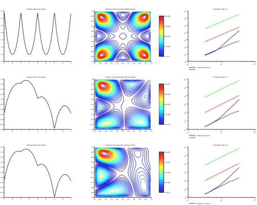
right column of Fig. 5.1, the convergence rates of standard finite-differences, discrete weighted means (DWM, see [15, 23, 52]) and (4.11) are compared. The red line, which indicates second-order accuracy, allows to easily check that both finite-differences and
Figure 5.1. Boundary data (left), pointwise errors (middle) and L2 convergence rates (right)
for finite-differences, discrete weighted-means and Steklov schemes. Red line indicates second order.
DWM are second-order methods, the size of the errors being very different, though. The Steklov scheme (4.11) behaves differently, in the sense that when the grid is coarse, it displays a fourth-order accuracy, which degrades to second-order when ∆x/ε goes below a certain value. This was to be expected as the modified Bessel functions behave like polynomials when their argument is very small (see also [52]). The DWM (or “tailored”, [23, 25]) methods, while being very accurate onE0,E1,E2,
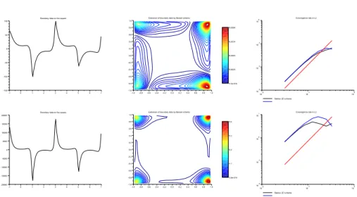
aren’t endowed with such a fast convergence property. Next, in order to illustrate the behavior for smaller ε’s, another (more complex) exact solution,
E3(x, y) = 0.5I2(r/ε)(sin 2θ + cos 2θ) +I3(r/ε) sin 3θ, ε = 0.1125 or 0.075,
was computed by both the DWM and Steklov schemes; see Fig. 5.2. By inspecting boundary data, one sees that a seemingly small variation in ε can produce a strong increase of the “spikes” at the Ω = (−1, 1)2 square’s corners where compatibility
conditions aren’t met. Indeed, for smaller ε, most of the numerical error accumulates in these regions. Both numerical methods appear to be similar and to converge at second order in L2when ∆x/ε is moderate; when ∆x/ε is bigger, the Steklov scheme
seems to behave a little bit better than the DWM (see Fig. 5.2, bottom).
5.2. Simple harmonic potential. Consider now an eigenvalue problem like,
−ε2∆u + V (x, y)u = λu, (x, y)∈ R2,
for which both eigenvalues λ’s and eigenfunctions are explicitly known when posed in the whole space, see Theorem 2.1. When 0 < ε is small enough, this explicit spectrum
Figure 5.2. Boundary data (left), pointwise errors (middle) and L2 convergence rates (right)
for Tailored (discrete weighted-means) and Steklov schemes. Red line again indicates second order.
Figure 5.3. Decay of L2norm (4.16): ε = 0.0066 (top, left), ε = 0.0033 (top, right), ε = 0.0022
(bottom, left) and ε = 0.0011 (bottom, right), for problem (5.1). Red line indicates third order.
can still be used in order to quantify pointwise errors of numerical schemes, even if the computational domain must be restricted to a bounded square inR2. Accordingly,
− ε2∆u + V (x, y)u = λu, V (x, y) = 0.25(|x − 0.5|2+|y − 0.5|2), (5.1)
is now posed in x, y∈ (0, 1)2 and its numerical spectrum is sought by both centered
finite-differences, and the “Steklov 2D scheme”. The Gaussian ground-state ϕε
to measure practically the decay of L2 norms (4.16) as ∆x → 0 for both numerical
algorithms: on Fig. 5.3, errors appear to decay at an order higher than 3 as soon as ∆x/ε is small enough, so that the grid can efficiently represent the numerical approximation. The decay corresponding to third order is illustrated by a red line on Fig. 5.3. To minimize the influence of truncating the computational domain without restricting too much the support of eigenfunctions, a convenient value of ε was experimentally found to be ε ≃ 0.007, with a grid 32 × 32. Pointwise relative
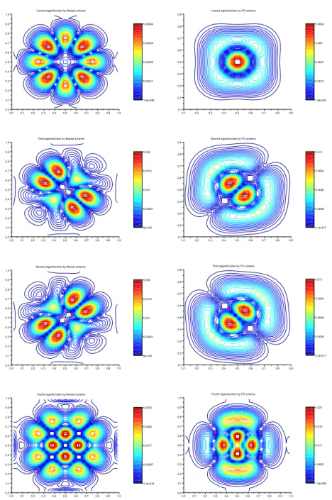
errors are displayed on Fig. 5.4: the left column displays relative errors coming from the “Steklov scheme” which suffer from less “mesh imprinting” (and are smaller) than the ones generated by standard centered finite differences (on the right column).
Remark 3. An inspection of Fig. 5.3 suggests that there are three different
regimes (instead of apparently two for finite differences) for the “Steklov scheme”: • a stiff one, ε ≪ ∆x, where the grid is really too coarse for a radial solution, • an intermediate one for which ε ≃ ∆x where L2 errors can decay very fast
(faster than order 4) compared to centered finite-differences,
• a fine-grid one, ε ≫ ∆x for which L2 errors decay at a rate close to order 3. 5.3. (A-)symmetric two-well potential. We illustrate this case with the
“Steklov 2D scheme” on the same computational grid, ε = 0.02 and the potentials,
V (x, y) = 1.01− exp ( − 30(|x − 0.65|2+|y − 0.35|2)) − exp(− 30(|x − 0.35|2 +|y − 0.65|2)), (V + δV )(x, y) = 1.01− exp ( − 30.5(|x − 0.65|2+|y − 0.35|2)) − exp(− 30(|x − 0.35|2+|y − 0.65|2)),
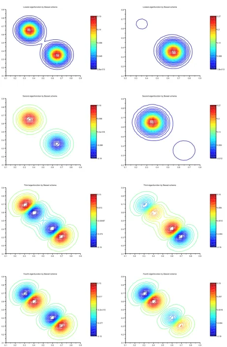
which share the same depth, but one is slightly wider than the other. On the left column of Fig. 5.5, usual symmetric eigenfunctions are generated by the scheme in presence of the double-Gaussian potential V (x, y), x, y ∈ (0, 1)2 with Dirichlet
boundaries and 25× 25 grid points. As expected, the ground state has a definite
sign, in accordance with the statements in Proposition 2. For the perturbed potential
V +δV , a quite different picture emerges as the perturbed ground state is now strongly
localized in the largest well, still being of a definite sign. The first perturbed excited state is localized in the narrow well and is endowed with small negative values. More excited eigenfunctions are less localized, but still, are never symmetric. Discrete orthogonality is checked in practice by looking at the L2 scalar products: it was
found to hold, up to machine accuracy (≃ 10−16) for both the five first unperturbed
eigenfunctions, and the perturbed ones (see also [37] for other benchmarks).
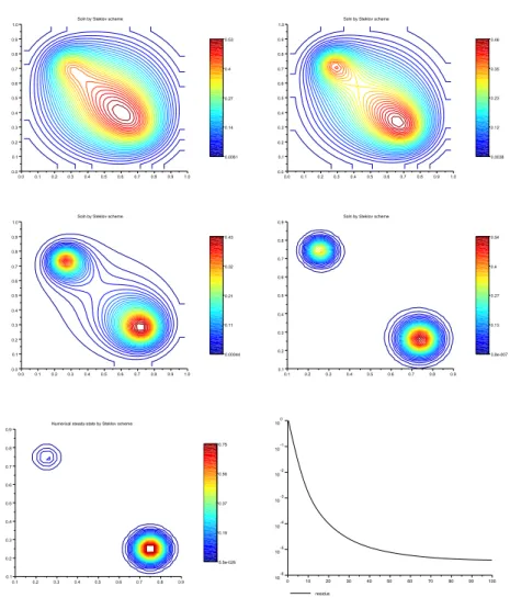
5.4. Time-dependent problem with two asymmetric wells. The 2D Steklov
scheme (4.11) can be recast as a time-marching algorithm, see [17, page 184], for
∂tu + ε2∆u + V (x, y)u = 0. (x, y)∈ (0, 1)2, (5.2)
with Dirichlet boundary conditions. The potential was chosen as,
V (x, y) = 0.95− exp (
− 10(|x − 0.75|2+|y − 0.25|2))
− exp(− 25(|x − 0.25|2+|y − 0.75|2)). (5.3)
Figure 5.4. Steklov scheme with Bessel functions (left) vs. centered FD (right).
displayed on Fig. 5.6. As expected from the spectral results derived in Section 3, the numerical solution accumulates more and more in the widest well, in agreement with the shape of the ground-state for asymmetric potentials, as displayed (for instance) on the right column of Fig. 5.5. The large-time behavior of (5.3) sees all the initial data’s mass accumulate in the widest well, the narrow one being depleted (at a rate which slows down as time grows). This is what is illustrated on the bottom line of
Figure 5.5. Steklov scheme: symmetric (left) vs. asymmetric (right) potential.
Fig. 5.6, where the numerical steady-state is shown to have nearly all its mass inside the widest well. Beyond T ≃ 50, the rate of change is very slow, though.
6. Conclusion and outlook. After recalling B. Simon’s “flea on the elephant”
phenomenon in 1D, see Fig. 1.1, analytical bounds were derived in Section 3 dealing with various perturbations of the classical quadratic harmonic potential; in particular,
Figure 5.6. Numerical solutions of time-dependent problem (5.2)–(5.3) at times T = 2, 3, 7, 20;
numerical steady-state at T = 100 (bottom, left) and corresponding L2 residues (bottom, right).
mass-accumulation in wider wells was justified with elementary arguments (see also [9, 20, 31, 45]). Then, in Section 4, the 2D scheme of [16, 17] is derived in a way which allows to produce error bounds for the constant coefficient case (see [52]). Such an algorithm, involving modified Bessel functions in 2D, is reminiscent of “discrete weighted means”, see [15, 23, 25, 40, 52]. Accordingly, the expected localization behavior is retrieved in Section 5, mostly for rough computational grids for which
ε/∆x≪ 1, see also [51], in both static and time-dependent contexts. As an outlook,
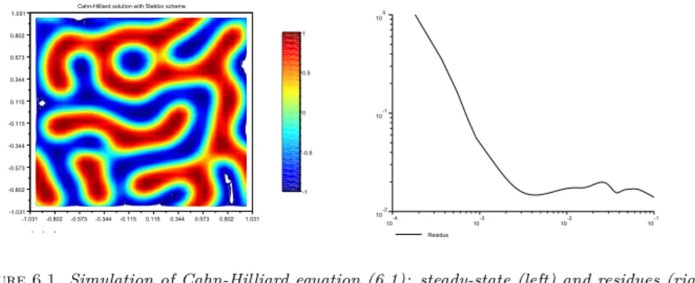
we outline an extension to a fourth-order Cahn-Hilliard [5, 12] type of equation:
∂tu− ∆
(
u(1− u2)− ε∆u )
= 0, x, y∈ (0, 1)2. (6.1) Following [50], we recast it as a system, except that, here, the nonlinearity is handled as a (locally) constant coefficient, (i.e. mass-conservation property may be lost)
∂tu + ε∆v− α2v = 0, v = ∆u, ∆
(
The “frozen parameter” α varies from disk to disk (see Fig. 4.1), α2(tn, xi±1 2, yj±12) = 1− u 2(tn, x i±1 2, yj±12).
Starting from random initial data belonging to the interval (−1, 1), and fixing ε =
Figure 6.1. Simulation of Cahn-Hilliard equation (6.1): steady-state (left) and residues (right).
0.002 with a 32× 32 computational grid, the expected phase-separation phenomenon, displayed on Fig. 6.1, was retrieved by using an explicit Euler time-integrator.
Acknowledgments. Enrique Zuazua’s research was supported by the Advanced
Grant DyCon (Dynamical Control) of the European Research Council Executive Agency (ERC), the MTM2014-52347 and MTM2017-92996 Grants of the MINECO (Spain) and the ICON project of the French ANR-16-ACHN-0014. L.G. thanks Profs. François Bouchut and Roberto Natalini for some technical discussions.
Appendix A. Elliptic regularity in a planar, square domain.
Let Ω = (0, 1)× (0, 1) be the (open) unit square and Γ stand for its boundary.
Consider the following strictly elliptic operator in Ω,
L[u] = −∆u + r(x, y)u = 0, u
Γ= g, r≥ 0, (A.1)
where both r and g are smooth functions. Because the domain is convex, but endowed with “corners”, the variational solution to (A.1) cannot be expected to be smoother than H2in general, see [21] and, e.g., [29, Theorem 4.3]. Refined regularity estimates
relying on Besov spaces theory were given in [8, Carollary 3.1]:
Theorem A.1. Let r ≡ 0 in (A.1), which reduces to Laplace’s equation, and g∈ Ws,p(Γ) with p < 2
1−ε and s∈ (1 − ε, 1): the harmonic solution u ∈ W
t,q(Ω) for
1
2 + s < q≤ p, 0 < t < s + 1
q.
If g∈ H1(Γ), then s = 1, p = 2 and u∈ Wt,q(Ω) with 1
3 < q≤ 2 and 0 < t < 1 + 1
q.
Another point of view consists in seeking under which restrictions on g the solution
u can be as smooth as if (A.1) was solved in a smooth domain. Following [33], let
u(x, y) =
3
∑
j ,ℓ=0
where ℓ = 0, 1, 2, 3 is the index of a vertex, and Λ stands for a linear functional acting on singular profiles ϕ localized around each corner of the domain Ω. These functional are linear combinations of differential operators acting on g, and the number of involved derivatives of g increases with respect to the index k. Accordingly, such a decomposition suggests that cancelling the Λ’s should ensure that u can become as smooth as its remainder v. These functionals were studied in many papers, after early works by Nicol’ski, Volkov, Fufaev, see [34, Chap. III]: for (A.1) and x = y = 0,
Λj(g) = d2jg dx2j(0 +, 0)− (−1)jd2jg dy2j(0, 0 +) (A.2) − j ∑ i=1 (−1)i−1 ∂ 2(j−i) ∂x2(j−i) ∂2(j−i) ∂y2(i−1) ( r(0, 0)u(0, 0)), j = 0, 1, 2, ...
Following [6, eq. (2.1)], see also [1, eq. (1.8-9)], the first ones in x = y = 0 are: Λ0(g) = g(0+, 0)− g(0, 0+), Λ1(g) = d2g dx2(0 +, 0) + d2g dy2(0, 0 +)− r(0, 0)u(0, 0), Λ2(g) = d4g dx4(0 +, 0)−d 4g dy4(0, 0 +) + ( ∂2 ∂x2 − ∂2 ∂y2 ) ( r(0, 0)u(0, 0)).
If all the derivatives of both g and r vanish close to each corner, (A.2) holds. Ac-cording to [24, Theorem 3.2] (see also [2, Theorem 2] and references therein), these “compatibility conditions” suffice for (A.1) to pass the Hölder regularity of g onto u:
Theorem A.2. Let g ∈ C2,λ on Γ minus its 4 vertices and Λℓ
0(g) = 0 for
ℓ = 0, 1, 2, 3: the solution of (A.1) u∈ C2,λ( ¯Ω). Moreover, for ¯Ω = [0, 1]× [0, 1],
u∈ C2k,λ( ¯Ω)⇔ g ∈ C2k,λ and Λℓ
j(g) = 0 for j≤ k and ℓ = 0, 1, 2, 3,
and if, under the same conditions, g∈ C2k+1,λ, then u∈ C2k+1,λ( ¯Ω).
Such regularity results can be formulated in other functional spaces, see for in-stance [35, 36]. There are several variants of this statement, like in [1, 10, 28, 33]:
Corollary 1. Assume that g ∈ C1,1 on Γ minus its 4 vertices and Λℓ
0(g) = 0
for ℓ = 0, 1, 2, 3, then the following second derivatives of u are bounded in Ω,
max( ∂ 2u ∂x2 , ∂2u ∂y2
)≤ C, but not the mixed one, ∂2u ∂x ∂y.
Restricting (A.2) to k = 0 only brings g(0+, 0) = g(0, 0+) at the vertex x = y = 0,
so that condition Λℓ
0(g) = 0 means that g is continuous at all four vertices of Ω. Appendix B. Trapezoidal rule and circular traces.
Let γRbe the “circular trace operator” Hs(R2)→ Hs− 1
2(0, 2πR) for which,
γR: u7→ γR[u], γR[u](θ) = u(R cos θ, R sin θ), f (x) = γR[u](Rθ),
where θ∈ (0, 2π). The proof of Lemma 5 is split into several steps:
• Being f : (0, T = 2πR) → R periodic, it rewrites as a Fourier series, f (x) =∑ k∈Z ˆ f (k) exp(ik2πx T ), ˆ f (k) = 1 T ∫ T 0 f (x) exp(−ik2πx T )dx.


![Figure 4.2. Counter-example of [4, Thm. 7]: polynomial (left) and its trace on C (0, ∆x) (right).](https://thumb-eu.123doks.com/thumbv2/123doknet/14643645.735636/17.918.147.608.160.319/figure-counter-example-thm-polynomial-left-trace-right.webp)