Characterisation of a new mobile absolute quantum gravimeter : application in groundwater storage monitoring

(1)

HAL Id: tel-03211175

https://tel.archives-ouvertes.fr/tel-03211175

Submitted on 28 Apr 2021

HAL is a multi-disciplinary open access archive for the deposit and dissemination of sci-entific research documents, whether they are pub-lished or not. The documents may come from teaching and research institutions in France or abroad, or from public or private research centers.

L’archive ouverte pluridisciplinaire HAL, est destinée au dépôt et à la diffusion de documents scientifiques de niveau recherche, publiés ou non, émanant des établissements d’enseignement et de recherche français ou étrangers, des laboratoires publics ou privés.

Characterisation of a new mobile absolute quantum

gravimeter : application in groundwater storage

monitoring

Anne-Karin Cooke

To cite this version:

Anne-Karin Cooke. Characterisation of a new mobile absolute quantum gravimeter : application in groundwater storage monitoring. Geophysics [physics.geo-ph]. Université Montpellier, 2020. English. �NNT : 2020MONTG043�. �tel-03211175�

(2)

THÈSE POUR OBTENIR LE GRADE DE DOCTEUR

DE L’UNIVERSITÉ DE MONTPELLIER

En Géosciences

École doctorale GAIA : Biodiversité, Agriculture, Alimentation, Environnement, Terre, Eau

Unité de recherche Géosciences Montpellier – UMR 5243

Présentée par Anne-Karin COOKE

Le 30 Octobre 2020

Sous la direction de Cédric CHAMPOLLION

Devant le jury composé de

Cédric CHAMPOLLION, Maître de conferences, Géosciences Montpellier Stéphane MAZZOTTI, Professeur, Géosciences Montpellier

Sylvain BONVALOT, Directeur de recherche, IRD, GET Toulouse Andreas GÜNTNER, Professor, GFZ, Potsdam University

Majken Caroline LOOMS ZIBAR, Associate Professor, Department of Geosciences and Natural Resource Management, University of Copenhagen

Directeur de thèse Examinateur Examinateur Rapporteur Rapportrice

Characterisation of a

new mobile absolute quantum gravimeter:

Application in groundwater storage monitoring

(3)

Acknowledgements

There are numerous people that deserve my uttermost gratitude. It is not possible to name everyone who contributed to this PhD thesis, but I have to start somewhere: First and foremost, I want to thank Cédric Champollion for the supervision, support and inspiration! In these three years, there was always an open space to think aloud, for discussion, the exchange of ideas, and fair communication. I am grateful for the trust and freedom. Then, I’d like to thank Nicolas Le Moigne for the technical support, advice, and critical thinking. I am grateful for all the inspiring discussions I had at Muquans: It was a pleasure to work with Camille Janvier and Pierre Vermeulen. I am impressed by the rigorous love for detail. Furthermore, my thanks go to Bruno Desruelle, Laura Antoni-Micollier, and Vincent Ménoret. Needless to say, everyone, I encountered at Muquans deserves my gratitude. I could learn a lot from everyone I met at Muquans and at Géosciences Montpellier.

Also, I’d like to thank Sébastien Merlet for the valuable input and critical view on the planning of experiments and feedback on the paper. I furthermore want to thank everyone else in my comité de suivi, Séverin Pistre, Jean Chèry, and Benoit Ildefonse, for the fruitful discussions. On other occasions, I had the chance to exchange thoughts on my work with Olivier Francis, Philippe Jousset, Marvin Reich, and many others.

In the ITN Enigma, I had the unique opportunity to meet many incredible researchers, in the network itself, the industrial partners, and the advisory board. Special thanks go to the aspiring, multicultural, and fun bunch of ESRs: We were a great team!

I am grateful for all the enriching experiences with people I met in Montpellier and Bordeaux: I am not going to name all the fellow PhD students, post-docs, senior researchers and technical staff I had the pleasure to interact with. Also at the Enigma summer school, at conferences, in seminars - the list is endless.

And I want to thank all my dear friends in France and around the world that accompanied me, old friends, that stayed by my side and new friends who came into my life during these three years.

Last but not least I want to express my tremendous gratitude towards my partner and my family, whose support and constant belief in me has been amazing. I am truly blessed to have you in my life!

All measurement presented here are from the Larzac observatory hosted by OSU OREME (http://www. oreme.org) and SNO H+ (http://hplus.ore.fr/). Larzac observatory and instrumentation are mainly funded by the CNRS INSU, ANR, Montpellier University, OZCAR, RESIF and Occitanie region. ENIGMA ITN has received funding from European Union’s Horizon 2020 research and innovation pro-gramme under the Marie Sklodowska-Curie Grant Agreement N°722028.

(4)

Synthesis

Quantum gravimeters provide the possibility of continuous, high-frequency absolute gravity monitoring while remaining user-friendly and transportable. This thesis assessed high precision performance mea-sures of the first commercial absolute quantum gravimeters AQG#A01 and AQG#B01 developed by Muquans. This was carried out in comparison with high precision absolute and relative gravimeters and additional geophysical and environmental data, in controlled conditions and experiments in view of future deployment in field conditions. Both AQG devices allow stable measurements of 𝑔 of several weeks. Significant drifts in time have not been observed. The two instruments have been transported and re-installed several times between sites and had been successfully applied in different conditions. The sensitivity of the AQG#A01 is better than 10 nm⋅s−2 _{after 24 h, which the AQG#B01 achieves}

after only one hour in a calm environment. For noisier environments, the sensitivity after one hour of the AQG#B01 is 20 to 30 nm⋅s−2_{. The repeatability of the AQG#B01 is reported as better than 50}

nm⋅s−2_{. Changes of instrument tilt and external temperature (20 - 30 °C) and combination of both did}

not influence the measurement of gravitational attraction. These results were also confirmed during two weeks of acquisition in an urban garage during which the measurement of 𝑔 remained unaffected by fast temperature changes. A rainfall event at the Larzac geodetic observatory caused a gravity increase of 100 nm⋅s−2_{in December 2019, which was detected with the AQG#B01 in agreement with the}

supercon-ducting relative gravimeter (GWR, iGrav#002) and corresponding Bouguer slab approximation. The potential gain in precision and time saved makes the AQG#B01 a promising instrument for e.g. large-scale gravity mapping. Such studies were formerly only feasible using a relative gravimeter that requires repeated acquisition loops and a reference absolute gravimeter for drift corrections. The AQG#B01 can be used without a reference instrument: It provides stable, repeatable measurements of absolute gravity while being transportable and user-friendly. Continuous monitoring at high precision allows for studies of high temporal resolution at different scales. The AQG#B01 would especially be suited for the moni-toring of transient mass changes at duration (e.g. a few weeks) that are too short to justify the effort of installing a stationary, superconducting gravimeter. To reliably detect transient phenomena, a drift-free and repeatable determination of 𝑔 is required for which e.g. spring relative gravimeters are not suitable. Some aspects are still under investigations, such as the potential effect of the sensor head’s orientation, the Coriolis effect, on the measurement of 𝑔 and the assessment of the accuracy regarding differences between the AQG#B01 and the absolute gravimeter (Micro-g LaCoste, FG5#228) that is used as a ref-erence. Time-lapse ground-based gravimetry is increasingly applied in subsurface hydrology to monitor water storage dynamics. The complementary spatial sensitivities of gravity and vertical gravity gradients (VGG) can be used to deduct the spatial characteristics of subsurface mass changes. VGG were estimated from one year of monthly relative gravity surveys on three different heights on three locations inside the Larzac observatory. The repeatability of VGG estimations was found to be better than 23 ± 9 E. The study suggests the influence of heterogeneous soil saturation patterns on VGG and the potential of dif-ferential VGG monitoring in resolving spatial mass distributions. Observed time-lapse, difdif-ferential VGG

(5)

List of Figures

2.1 Flowchart from tidal forces to tidal signal (from Agnew, 2015, p. 164). . . 7

2.2 FG5-X absolute gravimeter by Micro-g LaCoste Inc., 2020. . . 14

2.3 Scintrex CG5 and CG6 devices as part of RESIF’s GMob mobile gravimeter facility, in test at the Géosciences Montpellier laboratory (Bertrand, 2019). . . 16

2.4 Nb sphere kept stable within the magnetic field (from Hinderer et al., 2015; p. 67). . . 18

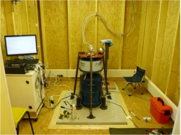
2.5 GWR iGrav-002 operating at the Larzac observatory, France, since 2011 (Le Moigne, 2019; RESIF). . . 19

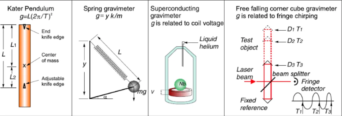
2.6 Working principles of a Kater pendulum, spring gravimeter, superconducting and free-fall corner cube gravimeter; from de Angelis et al., 2009, p. 8. . . 20

2.7 Conceptual differences between an optical interferometer (left) and an atom interferometer (right); from de Angelis et al, 2009, p. 2. . . 22

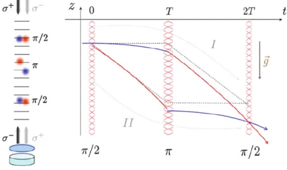
2.8 Schematic depiction of the atomic trajectories in an atom interferometer; from dos Santos and Bonvalot, 2016, p. 2. . . 23

2.9 Quantum gravimeter system requirements; from Geiger at al., 2020, p. 3. . . 25

3.1 The AQG-A01 on a tripod in the LNE laboratory (Trappes) on 01/10/2019. Photo: Cooke 29

3.2 Schematic overview of the functional subunits comprising of the sensor head, optics and electronics system as well as the aspect of supervision and monitoring. Muquans, 2017. . 30

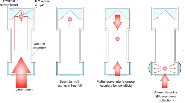
3.3 Schematic description of measurement sequence in the vacuum chamber. Source: Muquans. 31

3.4 Daily corrected gravity residuals (of the mean) in nm.s−2_{, for the AQG-A01 (red),}

iGrav-002 (black) and FG5-228 (blue) at the Larzac observatory 12/12/2018 - 08/01/2019 . . . 38

3.5 Daily corrected gravity residuals (of the mean) in nm.s−2_{, for the AQG-A01 (red),}

iGrav-002 (black) and FG5-228 (blue) at the Larzac observatory, 26/02 - 06/03/2019. . . 38

3.6 Daily averaged gravity residuals (of the mean) in nm.s−2_{, obtained with the AQG-A01 at}

Géosciences Montpellier, 25/03 - 24/04/2019 (panel (a)) and 06/05 - 03/06/2019 (panel (b)). . . 39

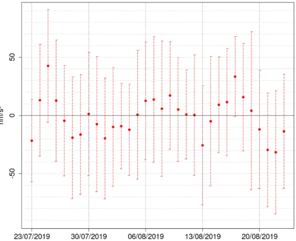
3.7 Daily gravity residuals from the mean in nm.s−2 _{obtained with the AQG-A01 at LNE}

(Trappes), 23/07 - 23/08/2019. . . 40

3.8 Allan deviation in nm.s−2_{for two series at each site, Montpellier and Larzac, respectively.}

Géosciences Montpellier March-April 2019 (red), May-June 2019 (blue). Larzac December 2018-January 2019 (black), February 2019 (lightgrey). Trappes July-August 2019 (orange). The horizontal blue dashed line shows the sensitivity benchmark of 10 nm.s−2_{, the dark}

green vertical dashed line signifies the integration period of 1 h, the light green line refers 24 h. . . 41

3.9 Allan deviation of 1-minute gravity residuals obtained with iGrav-002 at GEK (Larzac), 12/12/2018 - 08/01/2019. The horizontal blue dashed line shows the sensitivity benchmark of 10 nm.s−2_{, the dark green vertical dashed line signifies the integration period of 1 h, the}

light green line refers 24 h.. . . 42

3.10 Allan deviation at night (blue) and day (orange). AQG-A01 at GEK (Larzac) 12/12/2018 - 08/01/2019. . . 43

(10)

3.11 Allan deviation at night (blue) and day (orange). AQG-A01 at Géosciences Montpellier, 25/03 - 24/04/2019. . . 43

3.12 Allan deviation at night (blue) and day (orange). AQGA01 at Trappes 23/07/2019 -23/08/2019. . . 44

3.13 Allan deviation after 1 h of integration duration, calculated for each acquisition day. AQG-A01 at GEK (Larzac) 12/12/2018 - 08/01/2019. Public holidays are marked in light blue. 44

3.14 Allan deviation after 1 h of integration duration, calculated for each acquisition day. AQG-A01 at Trappes 23/07/2019 - 23/08/2019. Weekends are marked in light purple. . . 45

3.15 Allan deviation in nm.s−2_{after 1 h of integration duration, calculated for each acquisition}

day. AQG-A01 at Géosciences Montpellier on 25/03-24/04/2019. Weekends are marked in light purple. . . 45

3.16 Allan deviation in nm.s−2_{after 1 h of integration duration, calculated for each acquisition}

day. AQG-A01 at Géosciences Montpellier on 06/05-03/06/2019. Weekends are marked in light purple. . . 46

3.17 AQG-A01 hourly corrected gravity residuals (of the mean) in nm.s−2 _{at the Larzac}

obser-vatory, 12/12/2018 - 08/01/2019. Mean (red) and standard deviation over the whole series (dashed blue line). . . 47

3.18 AQG-A01 hourly averaged gravity residuals (of the mean) in nm.s−2_{, obtained with the}

AQG-A01 at Géosciences Montpellier, 25/03 - 24/04/2019. Mean (red) and standard deviation over the whole series (dashed blue line).. . . 48

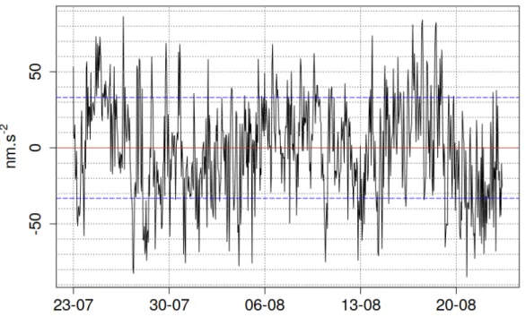
3.19 AQG-A01 hourly gravity residuals from the mean in nm.s−2 _{obtained with the AQG-A01}

at LNE (Trappes), 23/07 - 23/08/2019. Mean (red) and standard deviation over the whole series (dashed blue line). . . 48

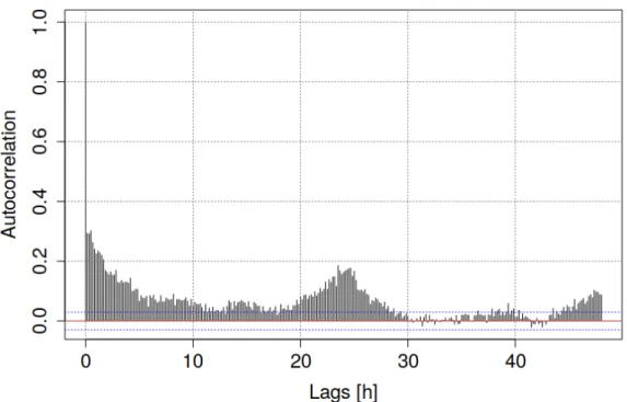
3.20 Auto-correlation of gravity residuals for a 48 h window. AQG-A01 at GEK (Larzac) 12/12/2018 - 08/01/2019. . . 49

3.21 Auto-correlation of gravity residuals for a 48 h window. AQG-A01 at Géosciences Mont-pellier during 25/03 - 24/04/2019 . . . 50

3.22 Auto-correlation of gravity residuals for a 48 h window. AQG-A01 at Géosciences Mont-pellier during 06/05 - 03/06/2019 . . . 50

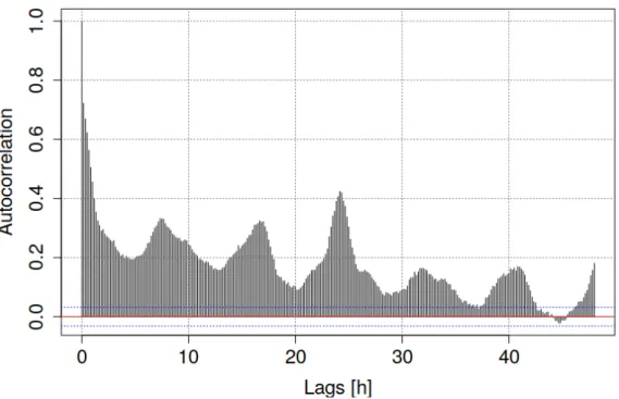
3.23 Auto-correlation of gravity residuals for a 48 h window. AQG-A01 at LNE (Trappes) 23/07 - 23/08/2019 . . . 51

3.24 Auto-correlation of seismic velocities in Northern direction at one Hz obtained from the STS-2 seismometer installed on the Larzac observatory site (RESIF). Time lags in hours. 12/2018 - 01/2019 . . . 52

3.25 Auto-correlation of vertical seismic velocities at 20 Hz obtained from the STS-2 seismome-ter installed on the Larzac observatory site (RESIF). Time lags in hours. 12/2018 - 01/2019 53

3.26 Auto-correlation of vertical vertical seismic velocities at 20 Hz filtred for frequencies lower than 1/60 Hz obtained from the STS-2 seismometer installed on the Larzac observatory

(11)

3.27 Power spectral density plot of vertical seismic velocities at 20 Hz obtained from the STS-2 seismometer installed on the Larzac observatory site (RESIF). Frequency in Hz. 12/12/2018 - 25/12/2019. Haned and Champollion, personal communication. . . 54

3.28 Power spectral density plot of vertical seismic velocities at 20 Hz obtained from the STS-2 seismometer installed on the Larzac observatory site (RESIF). Frequency in Hz. 25/12/2018 - 01/01/2019, Haned and Champollion, personal communication. . . 55

3.29 Correlogram of gravity residuals (’g’) and acquistion variables. Gravity residuals averaged over 10 minutes. AQG-A01 at GEK (Larzac) 12/12/2018 - 08/01/2019. Variables: ’hPa’ : atmospheric pressure, ’ext t’: external temperature, ’sh t’ : sensor head temp., ’vc t’: vacuum chamber temp., ’l t’: laser temp., ’tm t’ : tiltmeter temp., tilt X, tilt Y, ’sat’ : correction frequency offset of the saturated absorption spectroscopy, Laser polarisation angles phi and eta (rad) of the two lasers: cooler laser and repumper. . . 56

3.30 AQG-A01 at GEK (Larzac) 12/12/2018 - 08/01/2019. 10 minute gravity residuals from the mean in nm.s−2_{. Temperature residuals in °C from the mean: External (blue), laser}

(red), sensor head (green), vacuum chamber (orange) and tiltmeter (turquoise). . . 57

3.31 Correlogram of gravity residuals (’g’) and acquistion variables. Gravity residuals averaged over 10 minutes. AQG-A01 at GEK (Larzac) 26/02 - 06/03/2019. Variables: ’hPa’ : atmospheric pressure, ’ext t’: external temperature, ’sh t’ : sensor head temp., ’vc t’: vacuum chamber temp., ’l t’: laser temp., ’tm t’ : tiltmeter temp., tilt X, tilt Y, ’sat’ : correction frequency offset of the saturated absorption spectroscopy, Laser polarisation angles phi and eta (rad) of the two lasers: cooler laser and repumper. . . 58

3.32 Correlogram of gravity residuals (’g’) and acquistion variables. Gravity residuals averaged over 10 minutes. AQG-A01 at Géosciences Montpellier 25/03 - 24/04/2019. Variables: ’hPa’ : atmospheric pressure, ’ext t’: external temperature, ’sh t’ : sensor head temp., ’vc t’: vacuum chamber temp., ’l t’: laser temp., ’tm t’ : tiltmeter temp., tilt X, tilt Y, ’sat’ : correction frequency offset of the saturated absorption spectroscopy, Laser polarisation angles phi and eta (rad) of the two lasers: cooler laser and repumper. . . 59

3.33 Correlogram of gravity residuals (’g’) and acquistion variables. Gravity residuals averaged over 10 minutes. AQG-A01 at Géosciences Montpellier 06/05 - 03/06/2019. Variables: ’hPa’ : atmospheric pressure, ’ext t’: external temperature, ’sh t’ : sensor head temp., ’vc t’: vacuum chamber temp., ’l t’: laser temp., ’tm t’ : tiltmeter temp., tilt X, tilt Y, ’sat’ : correction frequency offset of the saturated absorption spectroscopy, Laser polarisation angles phi and eta (rad) of the two lasers: cooler laser and repumper. . . 60

3.34 Correlogram of gravity residuals (’g’) and acquistion variables. Gravity residuals averaged over 10 minutes. AQG-A01 at LNE Trappes 23/07/2019 - 23/08/2019. Variables: ’hPa’ : atmospheric pressure, ’ext t’: external temperature, ’sh t’ : sensor head temp., ’vc t’: vacuum chamber temp., ’l t’: laser temp., ’tm t’ : tiltmeter temp., tilt X, tilt Y, ’sat’ : correction frequency offset of the saturated absorption spectroscopy, Laser polarisation angles phi and eta (rad) of the two lasers: cooler laser and repumper. . . 61

3.35 Power spectral density plot of seismic velocities at 200 Hz obtained at Géosciences Montpel-lier. Frequency in Hz. 13/04 - 27/04/2020. Haned and Champollion, personal communication 62

(12)

3.36 Power spectral density plot of seismic velocities at 200 Hz obtained at Géosciences Montpel-lier. Frequency in Hz. 26/04 - 26/05/2020. Haned and Champollion, personal communication 63

3.37 Allan deviation for 10-minute data obtained with the AQG-A01 in 𝑛𝑚𝑠−2 _{obtained at}

LNE (Trappes), 23/07-23/08/2019. The horizontal blue dashed line shows the sensitivity benchmark of 10 𝑛𝑚𝑠−2_{, the dark green vertical dashed line signifies the integration period}

of 1 h, the light green one that of 24 h, pink refers to 7 days. . . 65

3.38 Acquisition protocol of VGG survey conducted with AQG-A01 on 67.2 cm tripod in LNE, Trappes, on 01/10/2019. The protocol allows for the assessment of several VGG throughout the day; including a comparison between a VGG based on 1 h measurement duration per height, respectively, and a 2h duration. The numbering of the gradients is shown at the specific result section. . . 66

3.39 Gravity residuals relative to the mean of the measurements at height zero (base tripod) (red dashed line). Measurements on an additional tripod (67.2 cm height difference). Data

obtained with the AQG-A01 at LNE (Trappes) on 01/10/2019 . . . 67

3.40 Vertical gravity gradients (VGG) in kE for 67.2 cm height difference obtained with the AQG-A01 at LNE (Trappes) on 01/10/2019. Gradient numbers refer to VGG estimated from gravity measurements based on one hour acquisition on each height (VGG nr. 1,2) or two hours (VGG nr. 3-6) (Figure 2.28, Table 2.2) . . . 68

3.41 CG6-120 gravity residuals for vertical gravity gradient estimation. Gravity residuals in nm.s−2_{, corrected for tidal effects and drift, obtained at at LNE (Trappes) on 01/10/2019.}

Colours indicate tripod height: ℎ₀ (black), ℎ₁(red), ℎ₂(purple), h3 (blue). . . 68

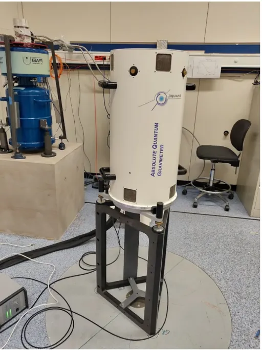
3.42 The AQG-B01 during operation in a garage in Montpellier 02/06/2020 - 17/06/2020. Photo: Cooke . . . 70

3.43 Auto-correlation function of AQG-B01 gravity residuals from the mean recorded during operation in a garage in Montpellier 02/06/2020 – 17/06/2020. Time lags in hours. . . 96

3.44 AQG-B01 gravity residuals from the mean recorded during operation in a garage in Mont-pellier 02/06/2020 – 17/06/2020. . . 97

3.45 Auto-correlation function of AQG-B gravity residuals from the mean recorded during op-eration. Correlogram of gravity residuals (’g’) and acquistion variables. Gravity residuals averaged over 10 minutes, obtained with AQG-B01 in a garage in Montpellier 02/06/2020 – 17/06/2020. Variables: ’hPa’ : atmospheric pressure, ’ext t’: external temperature, ’sh t’ : sensor head temp., ’vc t’: vacuum chamber temp., ’l t’: laser temp., ’tm t’ : tiltmeter temp., tilt X, tilt Y, ’sat’ : correction frequency offset of the saturated absorption spec-troscopy, Laser polarisation angles phi and eta (rad) of the two lasers: cooler laser and repumper. . . 98

3.46 Panel a: AQG-B gravity residuals from the mean recorded during operation in a garage in Montpellier 02/06/2020 – 17/06/2020. Panel b: external temperature in the garage recorded by AQG-B01 in °C. Panel c: Sensor head tilts in x (blue) and y (green) given in

(13)

3.47 Scintrex CG6-125 gravity residuals from the mean recorded during operation in a garage in Montpellier 02/06/2020 – 17/06/2020. One-minute CG6 data was corrected for ocean and solid Earth tides (tidal parameters for Géosciences Montpellier) and a linear drift of -166.483 ± 0.04 𝑛𝑚.𝑠−2_𝑑−1 _{subtracted. Mean (red) and standard deviation (blue, dashed}

line) for the entire series.. . . 100

3.48 Allan deviation of 10 min AQG-B01 data obtained during operation in a garage in Mont-pellier. The horizontal blue dashed line shows the sensitivity benchmark of 10 nm.s−2_{, the}

dark green vertical dashed line signifies the integration period of 1 h, the light green one that of 24 h.. . . 101

4.1 Scintrex CG5-1151 relative gravimeter on pillar 𝑝2 on height ℎ1in the Larzac observatory

in 2018. Photo: Cooke, 2018. . . 107

4.2 Modelled influence in E of the body mass of the operator on the vertical gravity gradient measurement as a function of distance in meters. . . 142

4.3 Larzac observatory concrete pillars during construction in 2011 (Photo: Le Moigne, 2011) 143

4.4 Gravity on surface of concrete pillar 1/2 at ℎ0 (0.261 m). Gravity residuals in nm.s−2

relative to mean gravity on the surface of 𝑝1,2. Gravity field caused by the mass of the

pillars 0-4. Centres of gravimeter measurement locations are marked as points. . . 143

4.5 Gravity on surface of concrete pillar 1/2 at ℎ1(0.85 m). Gravity residuals in nm.s−2relative

to mean gravity on the surface of 𝑝1,2. Gravity field caused by the mass of the pillars 0-4.

Centres of gravimeter measurement locations are marked as points. . . 144

4.6 Gravity on surface of concrete pillar 1/2 at ℎ₂ (1.436 m). Gravity residuals in nm.s−2

relative to mean gravity on the surface pf 𝑝_1,2. Gravity field caused by the mass of the pillars 0-4. Centres of gravimeter measurement locations are marked as points. . . 144

4.7 Gravity on surface of concrete pillar 3 at ℎ0(0.261 m). Gravity residuals in nm.s−2relative

to mean gravity on the surface of 𝑝3. Gravity field caused by the mass of the pillars 0-4.

to mean gravity on the surface of 𝑝₃. Gravity field caused by the mass of the pillars 0-4. Centres of gravimeter measurement locations are marked as points. . . 147

4.10 Gravity residuals in nm.s−2_{, relative to the average 𝑔}

0 of the six repeated measurements

obtained in September 2017. Adapted, after Ménoret et al., 2018, p. 8.. . . 148

4.11 Expected gravity in nm.s−2 _{caused by the mass of the pillars at exact measurement}

loca-tions for pillar 𝑝1 (darkblue), 𝑝2 (turquoise) and 𝑝3 (red). . . 149

4.12 Dots: Expected VGG in kE caused by the mass of the pillars and terrestrial gravity gradient (-3.0895 kE) at exact measurement locations for pillars 𝑝1 (darkblue), 𝑝2 (turquoise) and

𝑝3(red). Squares: Estimated VGG based on measurements obtained on 19/04/2018 for for

pillar 𝑝₁(darkblue), 𝑝₂(turquoise) and 𝑝₃(red). Error bars refer to the standard deviation of the three measurement loops, before drift correction. . . 150

(14)

4.13 Simulated gravity of a semi-infinite Bouguer slab in nm.s−2 _{on 0.5 m (black, dashed) and}

1.675 m height (black, continuous). (1) Slab of 10 m thickness. (2) Slab of 50 m thickness. Distance in meter from slab starting at x = 0 m. Density: 200 kg.m−3_._{. . . 154}

4.14 Simulated vertical gravity gradient of a semi-infinite Bouguer slab in nm.s−2 _{between 0.5}

m and 1.675 m height (red). Difference in E between VGG at 1.7 m horizontal distance (light blue). Slab of 10 m thickness. Distance in meter from slab starting at x = 0 m.

Density: 200 kg.m−3_. _{. . . 155}

4.15 Simulated vertical gravity gradient of a semi-infinite Bouguer slab in nm.s−2 _{between 0.5}

m and 1.675 m height (red). Difference in E between VGG at 1.7 m horizontal distance (light blue). Slab of 50 m thickness. Distance in meter from slab starting at x = 0 m.

Density: 200 kg.m−3_. _{. . . 155}

4.16 Horizontal distances between pillar measurement locations 𝑝₁, 𝑝₂ and 𝑝₃ (red). Distances in m. 𝑥_{𝑝1−𝑝2} = 1.3 m, 𝑥_{𝑝1−𝑝3} = 2.158 m, 𝑥_{𝑝2−𝑝3} = 1.7 m . . . 156

4.17 Panel (a): Transect crossing through the centre of each surface square of a 3D cubic heterogeneity. Panel (b): Diagonal transect. . . 157

4.18 Simulation of a 3D cubic heterogeneity pattern of 10 m edge length, respectively, with 200 kg.m−3 _{density. Gravity in nm.s}−2 _{on 0.5 m (black, dashed) and 1.675 m height (black,}

continuous). Vertical gravity gradient as the difference between both heights in E (red). Difference in E between VGG at 1.7 m horizontal distance (light blue). Gravity and VGG along a transect crossing through the centre of each surface square. Calculations at 1.7 m intervals.. . . 157

continuous). Vertical gravity gradient as the difference between both heights in E (red). Difference in E between VGG at 1.7 m horizontal distance (light blue). Gravity and VGG along a transect crossing the surface pattern diagonally. Calculations at 1.7 m intervals. . 158

continuous). Vertical gravity gradient as the difference between both heights in E (red). Difference in E between VGG at 1.7 m horizontal distance (light blue). Gravity and VGG along a transect crossing through the centre of each surface square. . . 159

continuous). Vertical gravity gradient as the difference between both heights in E (red). Difference in E between VGG at 1.7 m horizontal distance (light blue). Gravity and VGG along a transect crossing the surface pattern diagonally. . . 160

4.22 Rosette of fracture directions at the Larzac observatory site (Deville, 2013, adapted from Gerbaux, 2009).. . . 161

(15)

4.24 Simulation Gaussian (50 m) nr. 251 at 100 m depth. Cavity ’Cavité aven des dolines’ (Karst3D, 2019) . . . 162

4.25 Topography surrounding the Larzac observatory building (red square) in m.a.s.l. The 2D-geometry of the cavity is laid upon the map (black). . . 163

4.26 Residuals between the estimated vertical gravity gradients (VGG) in E for pillar 𝑝3(black)

and the annual mean of the estimated VGG on pillars 𝑝1and 𝑝2. Water level time series

in m for boreholes SD1 (brown), SD2 (orange) and SC1 (purple) the Larzac observatory, 2017-2019. . . 164

4.27 Conceptual model chart of observatory and potential local heterogenous soil water storages that supply the boreholes SC1 at 50 m, and SD1/SD2 at 20 m depth. Pillar 𝑝1,2is behind

𝑝₃ . . . 165

4.28 Cross-correlation between water level time series for borehole SD2 and estimated VGG on pillars 𝑝₁, 𝑝₂ and 𝑝₃. Blue dashed line: significance limit. . . 166

4.29 Simulated gravity in nm.s−2 _{and VGG in E for pillars 𝑝}

1 (darkblue), 𝑝2turquoise), 𝑝3 (red).168

4.30 Differences in E between the VGG simulated on the pillars. . . 168

6.1 ’Idealized representation of model assumed for the simulations. (a) Equipotentials and streamlines. (b) Cross section with darker shaded area corresponding to saturated portion of aquifer during hydraulic testing and lighter shaded area to dewatered portion. Gravity observations are made along the ground surface. For mathematical convenience, the coor-dinate origin is located along the axis of the pumping well at the initial static water level; and r and z are the unit directional vectors.’ Damiata and Lee, 2006, p.350 . . . 179

6.2 Procedure of determination of most suitable well test interpretation method, taking into account the hydrogeological context. From Gringarten et al., 2008, p. 47 . . . 182

6.3 Simulated pumping test based on the analytical Theis solution for unconfined, homoge-neous aquifers. Drawdown, corresponding gravity, and vertical gravity gradients at dif-ferent distances from the pumping well (located at 0 m). The analytical solution was transferred into a 3D model of 1 m cell size. Parameters: Specific yield 𝑆𝑦=0.1, pumping

rate of 3𝑖𝑚𝑒𝑠10−2_𝑚3_𝑠−1_{, pumping duration 7 days, initial head at surface. Two values}

of transmissivity were tested 𝑇1 =0.001 𝑚2𝑠−1 (black lines) and 𝑇1 =0.002 𝑚2𝑠−1 (blue

lines). Panel (a): Reduction in hydraulic head in meters, relative to surface. Panel (b): Gravity in nm.s−2 _{at 0.65 m measurement height. Panel (c): Vertical gravity gradients in}

E, based on from gravity difference at 0.65 and 1.32 m above surface. . . 186

6.4 Diagnostic plots for common hydrogeological settings: ’a Theis model: infinite two-dimensional confined aquifer; b double porosity or unconfined aquifer; c infinite linear no-flow boundary; d infinite linear constant head boundary; e leaky aquifer; f well-bore storage and skin effect; g infinite conductivity vertical fracture.; h general radial flow— non-integer flow dimension smaller than 2; i general radial flow model—non-integer flow dimension larger than 2; j combined effect of well bore storage and infinite linear constant head boundary’ (Renard et al., 2008; p.591) . . . 188

8.1 Porosity distribution: Surface view of simulation Gaussian (10m) nr. 251. . . 190

(16)

8.3 Porosity distribution: Surface view of simulation Exponential (10m) nr. 109. . . 191

8.4 Porosity distribution: Surface view of simulation Spherical (10m) nr. 94. . . 192

8.9 Porosity distribution: W-E profile of simulation Gaussian (10m) nr. 251.. . . 194

8.10 Porosity distribution: W-E profile of simulation Gaussian (50m) nr. 251.. . . 195

8.11 Porosity distribution: W-E profile of simulation Exponential (10m) nr. 109. . . 195

8.12 Porosity distribution: W-E profile of simulation Spherical (10m) nr. 94. . . 195

8.13 Porosity distribution: W-E profile of simulation Spherical (10m) nr. 144.. . . 196

8.17 Porosity distribution: N-S profile of simulation Gaussian (10m) nr. 251. . . 197

8.18 Porosity distribution: N-S profile of simulation Gaussian (50m) nr. 251. . . 197

8.19 Porosity distribution: N-S profile of simulation Exponential (10m) nr. 109. . . 198

8.20 Porosity distribution: N-S profile of simulation Spherical (10m) nr. 94. . . 198

8.25 Directional variogram analysis of surface layer of the simulation Gaussian (10m) nr. 251.. 200

8.26 Directional variogram analysis of surface layer of the simulation Gaussian (50m) nr. 251. 201 8.27 Directional variogram analysis of surface layer of the simulation exponential (10m) nr. 109.202 8.28 Directional variogram analysis of surface layer of the simulation spherical (10m) nr. 94. . 203

8.29 Directional variogram analysis of surface layer of the simulation spherical (10m) nr. 144. . 204

8.33 Directional variogram analysis of W-E profile of the simulation Gaussian (10m) nr. 251. . 208

8.34 Directional variogram analysis of W-E profile of the simulation Gaussian (50m) nr. 251. . 209

8.35 Directional variogram analysis of W-E profile of the simulation exponential (10m) nr. 109. 210 8.36 Directional variogram analysis of W-E profile of the simulation spherical (10m) nr. 94. . . 211

8.37 Directional variogram analysis of W-E profile of the simulation spherical (10m) nr. 144. . 212

(17)

8.44 Directional variogram analysis of N-S profile of the simulation spherical (10m) nr. 94. . . 219

(18)

List of Tables

3.1 Theoretically estimated precision on the vertical gravity gradient, given a height difference of 67.2 cm. . . 65

3.2 Large-scale repeatability: Δ𝑔 in nm.s−2 _{between Larzac and Montpellier obtained during}

surveys in 2019 with the FG5-228 and the AQG-A01 in 2019; AQG-B01 in 2020, respectively102

4.1 Differences in gravity between measurement locations on pillars 𝑝1, 𝑝2, 𝑝3 at heights ℎ0,

ℎ₁, ℎ₂. . . 148

4.2 Differences in gravity between measurement locations on pillars 𝑝₁, 𝑝₂, 𝑝₃ at heights ℎ₀, ℎ₁, ℎ₂. . . 151

(19)

Résumé

La gravimétrie est l’étude des variations spatiales et temporelles du champ de gravité terrestre, ces variations pouvant être liées à des changements de distribution de masse étudiés dans diverses disciplines des sciences de la Terre. Les applications incluent la géodésie et la géodynamique à grande échelle comme la tectonique et la subsidence lent (Camp et al. (2011); Hwang et al. (2010)) ainsi que incluant la déformation de la croûte et le soulèvement isostatique glaciaire (Mazzotti et al. (2011); Olsson et al. (2019)). La gravimétrie s’est par ailleurs avérée être un outil d’évaluation des aléas naturels tels que le suivi de l’activité volcanique (Bonvalot, Diament, and Gabalda (1998), Carbone et al. (2017)), la cartographie des vides souterrains ou l’étude des tremblements de terre (Imanishi (2004)). Les applications dans le domaine de l’énergie et des ressources comprennent les champs géothermiques (Pearson-Grant, Franz, and Clearwa-ter (2018)), les réservoirs de stockage de CO₂ (Sugihara et al. (2017)) ou les installations de recharge artificielle des eaux souterraines (Kennedy, Ferré, and Creutzfeldt (2016)). Les méth-odes gravimétriques trouvent en outre une application dans le contexte de l’exploration et de la prospection pétrolières et minérales (par exemple Ferguson et al. (2007); Hinze, Von Frese, and Saad (2013)). En hydrologie, la mesure de la gravité offre des possibilités de surveiller la dynamique de stockage des ressources en eaux souterraines locales et à l’échelle du paysage (par exemple Creutzfeldt et al. (2008); Creutzfeldt et al. (2010); Jacob et al. (2010); Hector et al. (2014); Hector et al. (2015); Fores, Champollion, Moigne, Bayer, et al. (2016); Güntner et al. (2017)) et même les taux d’évapotranspiration (Van Camp et al. (2016)). Les applications et les

domaines de recherche sur la gravité active ont été largement examinés par Crossley, Hinderer, and Riccardi (2013) et Camp et al. (2017).

Les gravimètres sont des appareils qui mesurent l’attraction gravitationnelle 𝑔 à la surface de la Terre. Les gravimètres peuvent être caractérisés par leurs performances de mesure. La répétabil-ité d’une mesure fait référence à l’accord entre des mesures répétées et est généralement évaluée en effectuant plusieurs changements d’emplacement répétés entre les mesures. La sensibilité (ou précision) d’un gravimètre est une incertitude relative et se réfère au plus petit changement d’accélération gravitationnelle que le gravimètre est capable de détecter. Nous parlons de sta-bilité comme de l’absence de dérive instrumentale significative dans le temps ou de bruit corrélé. La précision d’une mesure de gravité décrit dans quelle mesure elle peut être considérée comme correcte en termes absolus et fait référence à l’incertitude d’une mesure par rapport à un étalon absolu (Niebauer (2015)).

Les gravimètres relatifs détectent l’attraction gravitationnelle indirectement en mesurant la force nécessaire pour annuler la gravitation en stabilisant une masse d’essai et sont utilisés pour surveiller les changements de gravité relative dans le temps ou dans l’espace. Ces dispositifs

(20)

montrent des dérives qui peuvent devenir importantes en quelques jours (gravimètres à ressort) ou quelques mois (gravimètres supraconducteurs) (Camp et al. (2017)). Les gravimètres relatifs nécessitent un étalonnage régulier avec des gravimètres absolus comme stations de référence et des mesures répétées en boucle ou absolues pour éliminer les dérives dans les levés de terrain (Hector and Hinderer (2016); Kennedy and Ferré (2015)). Ils peuvent être sensibles aux

change-ments de température (par exemple avec un gravimètre à ressort relatif comme dans Fores, Champollion, Moigne, and Chery (2016)). Les gravimètres relatifs les plus sensibles sont les gravimètres supraconducteurs et atteignent une haute précision d’environ 0,1 𝑛𝑚.𝑠−2 _{tout en}

mesurant en continu à une fréquence d’échantillonnage de 1 Hz. Ils sont basés sur la lévitation magnétique au lieu d’un ressort mécanique (Hinderer, Crossley, and Warburton (2015)).

Les gravimètres absolus estiment la norme de l’accélération gravitationnelle 𝑔 en chute libre verticale dans le vide (Niebauer et al. (1995)). Les gravimètres absolus sont principalement basés sur un rétroréflecteur cubique en chute libre dans une chambre à vide avec une incertitude instrumentale de l’ordre de quelques dizaines de 𝑛𝑚.𝑠−2 _{(Niebauer (2015)). Les gravimètres}

absolus actuellement disponibles ne sont pas adaptés à une surveillance continue en raison de pièces mécaniques à durée de vie limitée. Cela limite le nombre d’expériences de chute libre et nécessite une maintenance fréquente des instruments. Leur fonctionnement nécessite générale-ment un niveau de compétence technique élevé et ils ne peuvent être mis en oeuvre par un non-spécialiste.

La détection quantique offre de nouvelles possibilités pour la mesure de l’inertie et le développe-ment de gravimètres quantiques absolus. Le principe général de mesure d’un gravimètre quan-tique absolu (AQG) est celui de l’interférométrie matière-ondes ((Peters, Chung, and Chu (2001)); Merlet et al. (2010)). Les atomes peuvent être exploités comme masses de test ainsi que comme outil pour mesurer le chemin parcouru afin de détecter la gravité (Peters, Chung, and Chu (2001)). Réalisation de laboratoire, le gravimètre à atome froid (CAG) développé au LNE-SYRTE dans le cadre de la balance Kibble a démontré des performances inédites tant en sensibilité qu’en précision. Il a depuis participé à International Comparisons of Absolute Gravimeters (ICAG) montrant une meilleure sensibilité à court terme que les gravimètres ab-solus et un budget de précision rigoureusement quantifié (Jiang et al. (2012); Francis et al. (2013); Gillot et al. (2014)). De nombreux instituts de recherche et entreprises privées travail-lent sur différentes réalisations de gravimètres à atomes froids (Geiger et al. (2020)) comme GAIN (Allemagne; Hauth et al. (2013)) ou WAG-H5-1 (Chine; Huang et al. (2019)). Une manipulation robuste des atomes, étape cruciale vers la réalisation d’un instrument de terrain,

(21)

un fonctionnement avec un seul faisceau optique, et conduisant à une mise en œuvre compacte (après Bodart et al. (2010)). Un examen exhaustif de l’état de l’art des capteurs à inertie

gravi-tationnelle à atome froid, des différents types de capteurs, des applications et des différences de performances a été fourni par Geiger et al. (2020). Le premier gravimètre disponible dans le commerce (AQG#A) basé sur cette technologie a été développé par Muquans. La conception compacte a permis un instrument mobile qui ne nécessite pas de formation spéciale pour mise en oeuvre. Les progrès de la correction à la volée des effets externes ont contribué à la création d’un instrument compact et stable de haute sensibilité mesurant à une fréquence d’échantillonnage de 2 Hz. Une stabilité meilleure que 10 𝑛𝑚.𝑠−2 _{pendant un mois de fonctionnement a été observée,}

et la répétabilité de l’instrument a été préalablement quantifiée pour être du même ordre de grandeur (Ménoret et al. (2018)) pendant 24 h.

Conclusion

L’objectif principal de cette thèse était l’évaluation des mesures de performance de haute pré-cision des gravimètres quantiques absolus en comparaison avec des gravimètres absolus et re-latifs de haute précision et des données géophysiques et environnementales complémentaires. Deux gravimètres quantiques absolus, les Muquans AQG#A01 et AQG#B01, ont été évalués en se concentrant sur des mesures de performance importantes: précision, sensibilité, stabilité et répétabilité. Des mesures de plusieurs semaines ont été réalisées à trois endroits différents: l’observatoire du Larzac, Géosciences Montpellier et Trappes (près de Paris).

La characterisation de l’AQG#B01 a été réalisé dans des conditions contrôlées et via de nom-breuses expériences en vue d’un déploiement futur sur le terrain. Les principaux objectifs de cette étude sont d’évaluer la stabilité et la répétabilité du premier gravimètre quantique absolu de terrain en vue d’un déploiement futur en tant que gravimètre de terrain pour des applica-tions hydrogéophysiques. L’évaluation se fait lors de mesures et d’expériences en continu (impact d’orientation ou de transport) en comparaison avec des gravimètres absolus et relatifs. La sen-sibilité aux changements d’inclinaison et de température ainsi que l’interaction entre les deux sont d’une importance cruciale pour évaluer l’aptitude de l’AQG#B01 en tant qu’instrument de terrain. Sa sensibilité aux variations de température ambiante est évaluée en effectuant des tests dans un environnement contrôlé. Enfin, des recommandations sont présentées pour l’utilisation future de l’AQG#B01 dans des expériences sur le terrain.

De l’expérience de ces expériences, on peut conclure ce qui suit:

• Un arrêt, un démontage, un transport et un redémarrage complet réussis ont été obtenus avec les deux instruments lors de plusieurs déplacements

(22)

AQG-A01

En complément de l’étude de Ménoret et al. (2018), les résultats supplémentaires suivants ont été obtenus pour l’AQG#A01:

• Dans un environnement à faible bruit (Larzac), l’AQG-A01 atteint une sensibilité inférieure à 10 nm⋅s−2 _{après 24 h d’intégration de données}

• La sensibilité et la stabilité montrent une forte variabilité due à des oscillations subjour-nalières

• Ces oscillations sont susceptibles d’être liées à l’instabilité laser, mais la corrélation n’est pas systématiquement reproductible sur tous les sites d’étude

• Estimation du gradient de gravité vertical (VGG) basé sur des mesures sur trépieds de deux hauteurs différentes avec l’AQG-A01 moins précis que l’estimation VGG avec un gravimètre relatif CG6

AQG-B01

Sur la base de l’expérience acquise avec l’AQG#A01, la version de suivi sur le terrain (AQG#B01) comprend des améliorations considérables en termes de sensibilité et de stabilité.

La caractérisation de l’AQG#B01 pour les applications sur le terrain s’est concentrée sur les conditions potentielles du terrain ayant un impact sur la température, l’inclinaison et l’orientation de la tête du capteur.

Les principales conclusions sont les suivantes:

• Dans les environnements à faible bruit (observatoire du Larzac), l’AQG-B01 a montré une sensibilité de 10 nm⋅s−2 _{après 1 h}

• La sensibilité après 24 h d’intégration des données est proche de celle de l’iGrav-002 à l’observatoire du Larzac

• Dans les environnements bruyants (Montpellier), la sensibilité est comprise entre 20 et 30 nm⋅s−2 _{après 1 h}

• La répétabilité a été quantifiée à 3 nm⋅s−2 _{avec un écart type de 25 nm⋅s}−2

• Surveillance des changements de masse hydrologique: Accord entre les résidus grav-imétriques mesurés avec l’iGrav et l’AQG-B01

(23)

ex-• Aucun effet d’une interaction potentielle entre la température et l’inclinaison de la tête du capteur sur la mesure de 𝑔 observée

• Fonctionnement fiable pendant deux semaines dans un garage, aucun impact observé des changements rapides de température, des niveaux de bruit accrus ou des mouvements d’air lors de l’ouverture des portes de garage

• Montpellier: Δ𝑔 entre AQG-B01 et FG5-228 était de 44 nm⋅s−2 _{avec un écart type de 66}

nm⋅s−2 _(𝑔

𝐴𝑄𝐺−𝐵< 𝑔𝐹 𝐺5)

• Larzac: Δ𝑔 entre AQG-B01 et FG5-228 était de 110 nm⋅s−2 _{avec un écart type de 31}

nm⋅s−2 _(𝑔

𝐴𝑄𝐺−𝐵> 𝑔𝐹 𝐺5)

Prochaines étapes proposées

Des informations pratiques pourraient être tirées de la caractérisation des instruments présen-tée dans cette thèse. Cependant, l’étude n’est pas exhaustive, car l’évaluation du budget d’incertitude d’un gravimètre reste une tâche complexe. Dans un proche avenir, les tests suivants sont importants:

• L’impact de l’orientation de la tête du capteur (effet Coriolis) sur la mesure de 𝑔 doit être approfondi

• Le suivi de plusieurs mois pour évaluer la stabilité à long terme

• La répétabilité et la transportabilité doivent être répétées: déplacements supplémentaires entre Montpellier et le Larzac (et autres lieux)

Études appliquées potentielles

Le gain potentiel de précision et de gain de temps fait de l’AQG#B01 un instrument prometteur pour, par exemple, la cartographie gravimétrique à grande échelle. Ces études n’étaient aupar-avant réalisables qu’en utilisant un gravimètre relatif qui nécessite des boucles d’acquisition répétées et un gravimètre absolu de référence pour les corrections de dérive. L’AQG#B01 peut être utilisé sans instrument de référence: il fournit des mesures stables et reproductibles de la gravité absolue tout en étant transportable et ergonomique. Surveillance temporelle des change-ments de masse, par exemple des signaux hydrogéophysiques, sur d’autres sites, sont envisagés. La surveillance continue à haute précision permet des études de haute résolution temporelle à différentes échelles. L’AQG#B01 serait particulièrement adapté pour la surveillance des change-ments de masse transitoires à des durées (par exemple quelques semaines) trop courtes pour justifier l’effort d’installation d’un gravimètre supraconducteur. Pour détecter de manière fiable les phénomènes transitoires, une détermination sans dérive et répétable de 𝑔 est nécessaire pour

(24)

laquelle les gravimètres à ressort ne conviennent pas.

Surveillance des gradients verticaux de gravité

Lier les caractéristiques spatiales et temporelles des observations gravimétriques aux phénomènes et caractéristiques géophysiques est au cœur de la discipline. La cartographie des anomalies de gravité spatiale peut être utilisée pour détecter les contrastes de densité du sous-sol tels que déployés dans l’exploration et la prospection pétrolières et minérales (par exemple Ferguson et al. (2007); Hinze, Von Frese, and Saad (2013)) ou pour la détection de dépressions souterraines (Jacob et al. (2018)). Les résidus temporels subsistent après correction des séries chronologiques gravimétriques pour les effets connus tels que les signaux de marée et les variations de pression atmosphérique. Ces résidus peuvent être attribués à des changements de masse locaux (Crossley, Hinderer, and Riccardi (2013); Camp et al. (2017)).

Les effets hydrologiques globaux et locaux de la gravité sur les observations gravimétriques sont causés par la déformation de la croûte et l’attraction newtonienne des masses d’eau (Llubes et al. (2004); Harnisch and Harnisch (2006); Linage, Hinderer, and Rogister (2007); Neumeyer et al. (2008); Longuevergne et al. (2009), Wziontek et al. (2009)). Les signaux hydrologiques dans les données gravimétriques au sol se produisent principalement à des échelles de temps et de longueur intermédiaires (heures en années, mètres en kilomètres). De plus, ils peuvent être fortement dépendants du site et complexes à déterminer (Harnisch and Harnisch (2006)).

L’hydrogravimétrie comme l’une des méthodes d’exploration hydrogéophysique émergentes four-nit une approche spatialement intégrative et non invasive pour l’imagerie souterraine. La prin-cipale caractéristique des mesures gravimétriques est leur nature intégrant la profondeur qui comprend les contributions des changements de masse locaux et distants. Cela a trouvé son ap-plication dans les bilans massiques contraignants pour les estimations du stockage total de l’eau (TWS). Il facilite la caractérisation des écoulements souterrains dans les aquifères hétérogènes où les mesures ponctuelles hydrologiques classiques manquent de représentativité (Binley et al. (2015)). Par exemple, dans les karsts fortement hétérogènes, les niveaux d’eau provenant de

forages uniques peuvent ne pas être représentatifs de la dynamique globale de la teneur en eau souterraine (Hartmann et al. (2014)). La gravimétrie au sol offre un outil important pour détecter les changements de masse locaux qui sont trop faibles pour la gravimétrie spatiale à grande échelle mais trop éloignés ou répartis dans l’espace pour être représentés dans des mesures de points hydrologiques, comme le montrent des études hydrogravimétriques récentes dans les régions karstiques ( Mazzilli et al. (2012); Mouyen et al. (2019)).

(25)

masses telles que la déduction de la profondeur et les informations directionnelles. Malgré ces défis, la séparation et l’identification des signaux peuvent être obtenues par l’inclusion d’autres techniques géophysiques, géodésiques ou hydrologiques et l’analyse de la signature temporelle du changement de gravité. Cette hydrogravimétrie hybride accélérée est ainsi capable de con-traindre et de quantifier les changements de stockage de l’eau (WSC) et de séparer les zones contributives et les processus impliqués (Naujoks et al. (2007); Naujoks et al. (2010)), tels que les précipitations (Meurers, Camp, and Petermans (2007), Delobbe et al. (2019)), l’humidité du sol (Krause et al. (2009)), l’évapotranspiration (Van Camp et al. (2016)) et le ruissellement et les rejets de surface (Lampitelli and Francis (2010); Creutzfeldt et al. (2013), Piccolroaz et al. (2015)), les changements de stockage de l’eau du captage (Hasan et al. (2008)) Hector et al. (2014), Hector et al. (2015); Güntner et al. (2017)) ou pour surveiller les installations de recharge artificielle des eaux souterraines (Davis, Li, and Batzle (2008); Kennedy, Ferré, and Creutzfeldt (2016)).

L’effet gravitationnel des changements de masse d’eau (par exemple un événement de précipita-tion) est généralement simplifié sous la forme d’une dalle homogène et infinie (plaque de Bouguer) d’une colonne d’eau. Cette hypothèse peut ne pas s’appliquer dans les aquifères hétérogènes (par exemple les karsts). Le signal de gravité intégrant la profondeur n’inclut pas d’informations sur la distribution spatiale des masses. Contrairement aux mesures de l’intensité du champ gravita-tionnel, le gradient de gravité vertical (VGG) est sensible aux changements de masse latéraux. Les sensibilités spatiales complémentaires de la gravité et des VGG peuvent être utilisées pour déduire conjointement les caractéristiques spatiales des changements de masse dans le sous-sol. Dans cette étude, nous avons évalué la précision de la surveillance des VGG à l’aide de grav-imètres de terrain relatifs placés sur des trépieds dans un cadre d’observatoire contrôlé et avons relié nos résultats au contexte hydrogéologique du site d’étude. Les VGG ont été estimés à partir de relevés mensuels de gravité relative sur trépieds de différentes hauteurs sur trois piliers en béton de l’observatoire géodésique du Larzac dans le sud de la France, entre décembre 2017 et novembre 2018. La répétabilité des estimations VGG basées sur cette méthode a été estimée à 23 ± 9 E. Des changements de VGG de ∼ 80 Eotvos (1 E = 10−9_s−2_{) en un an sur l’un}

des emplacements de mesure ont été observés. En l’absence d’autres changements de masse, les changements de VGG étaient liés aux sources possibles de changement de stockage d’eau à proximité. Premièrement, l’impact de l’effet parapluie (protection du bâtiment contre les pré-cipitations) a été testé comme une source potentielle de changements VGG et s’est avéré limité à quelques E. Deuxièmement, les distributions possibles de porosité souterraine ont été générées dans la simulation stochastique géostatistique et sélectionnées pour obéissez aux changements observés de gravité et de VGG ainsi qu’aux différences entre les emplacements de mesure. Les

(26)

données conjointes de gravité et de gradient de gravité ont réduit la gamme de simulations co-hérente avec les données. Nous discutons en outre du potentiel des mesures de VGG comme une nouvelle technique potentielle pour résoudre spatialement les changements de masse dans un contexte hydrogéologique.

L’estimation du gradient de gravité vertical basée sur des boucles répétées réalisées avec un gravimètre à ressort relatif sur trépied est une méthode longue qui ne permet pas une résolu-tion temporelle élevée. La mesure prend environ une journée de travail et un post-traitement approfondi est nécessaire pour une correction adéquate des dérives et autres effets. Nous avons quantifié la répétabilité des estimations VGG à 23 ± 9 E. Pour la différence de hauteur de 117,5 cm entre les mesures, 20 E se réfère à 23,5 nm⋅s−2 _erreur.

Les simulations géostatistiques stochastiques réalisées montrent d’éventuelles distributions spa-tiales des propriétés souterraines qui conduiraient à des différences de VGG entre les piliers de plusieurs dizaines de E tout en limitant les variations de gravité à quelques dizaines de nm⋅s−2_.

Nous avons supposé une plage de porosité en cohérence avec les diagraphies de forage et les résultats d’inversion des études hydrogéophysiques précédentes. Cette étude a montré que la surveillance des VGG est sensible à une hétérogénéité souterraine locale qui autrement ne serait pas visible dans la série gravimétrique seule. Les gradients de gravité permettent d’accéder à l’hétérogénéité de la surface et à l’emplacement des changements de masse. Contrairement aux mesures gravimétriques uniques qui représentent des mesures intégratives de profondeur, les gradients de gravité donnent accès à des informations au-delà des limites de l’approximation de plaque de Bouguer classiquement utilisée en hydrogravimétrie. Nous recommandons, cepen-dant, d’affiner d’abord les paramètres de simulation sur la base de variogramme directionnel et d’inversion avec des données fournies par d’autres méthodes d’imagerie géophysique. Afin de mieux comprendre les processus souterrains du site du Larzac qui montrent potentiellement une influence détectable sur les estimations VGG, nous suggérons une approche conjointe de surveillance supplémentaire de la teneur en eau du sol, de simulations stochastiques affinées et de développement de modèles hydrologiques. Des études répétées de tomographie de résistivité électrique ajouteraient des informations sur les changements de saturation saisonniers à partir desquels d’autres modèles de variogramme directionnel pourraient être ajustés, ce qui limiterait les simulations géostatistiques et augmenterait le réalisme hydrogéologique. La dynamique du stockage de l’eau karstique et la distribution de la porosité ont été résolues par une surveillance ERT à long terme (Watlet et al. (2018)). Des profils ERT supplémentaires à différents an-gles du bâtiment pourraient aider à identifier l’anisotropie locale en appliquant l’ajustement de

(27)

L’observatoire du Larzac offre des conditions favorables pour la surveillance gravimétrique en rai-son de l’environnement peu bruyant, de la température contrôlée et d’un suivi hydrogéophysique supplémentaire sur le site. Cependant, son aptitude à la comparaison gravimétrique en termes de précision est limitée par la variabilité spatiale et temporelle du champ gravitationnel local. Les piliers en béton dépassent de 0,5 m de la surface du sol, provoquant des gradients de gravité verticaux non linéaires (courbure) dans les 2 premiers mètres au-dessus de la surface du pilier. Les différences entre les courbures observées et simulées causées par les piliers en béton suggèrent l’impact d’une hétérogénéité souterraine supplémentaire. La cartographie précise de la courbure est limitée par la sensibilité de la méthode d’estimation VGG disponible. Il est recommandé d’effectuer des comparaisons gravimétriques dans les observatoires où les piliers sont idéalement intégrés dans une plaque de béton plus grande et plate. Des mesures avec plusieurs déplace-ments entre les piliers de l’observatoire du Larzac sont recommandées. De plus, l’observatoire du Larzac est exposé aux changements d’humidité du sol dans la zone non saturée environnante. Leur impact sur les mesures de gravité en raison de l’incertitude liée à la correction VGG peut être potentiellement important. En un mot, le suivi des VGG peut être résumé dans les points suivants.

Variations de VGG temporelles observées

• Un an de levés gravimétriques mensuels réalisés avec un gravimètre relatif CG5 sur trois hauteurs différentes sur trois piliers

• Répétabilité de l’estimation VGG quantifiée à 23 ± 9 E

• 80 E changement observé sur le pilier du point de mesure 𝑝₃

• Les VGG sur les piliers 𝑝₁ et 𝑝₂ ne montrent pas de tendances significatives

• Plusieurs dizaines d’E de bruit VGG time-lapse peuvent conduire à des décalages de gravité non négligeables lors de la comparaison de gravimètres

Surveillance différentielle VGG comme méthode hydrogéophysique

Les changements observés de VGG ont été étudiés à la recherche du changement de masse correspondant.

• Impact simulé de l’effet parapluie (zone de construction protégeant le sous-sol des précipi-tations) sur le VGG de l’ordre de quelques E

• L’impact de l’hétérogénéité du sous-sol a été étudié à l’aide d’une simulation géostatistique stochastique

(28)

nombre de réalisations souterraines simulées appropriées

• Aucune corrélation significative entre les propriétés simulées du sous-sol et les structures géologiques existantes (cavité, orientation de la fracture)

• Effet de la topographie locale sur VGG estimé négligeable

• Des simulations simplifiées concernant les variations de stockage de l’eau à l’emplacement de deux forages à 20 m de profondeur montrent des changements de gravité et de VGG dans l’ordre de grandeur des changements observés

Prochaines étapes

• Simulations raffinées avec des paramètres d’anisotropie mieux contraints, basées sur des mesures de saturation supplémentaires

• Recherches complémentaires sur l’impact de la dynamique temporelle des stockages souter-rains

• Potentiel d’estimation VGG avec AQG-B: surveillance plus efficace, sensibilité attendue 21 E et répétabilité de 6,3 ± 53 E

Un autre objectif de cette thèse était le développement de nouvelles méthodes de gravimétrie dans le contexte de l’hydrologie. Dans cette thèse, la surveillance time-lapse des VGG a été testée à l’aide de gravimètres relatifs disponibles. La précision et les limites attendues de la méthode ont été évaluées. L’étude suggère l’influence de l’hétérogénéité dans la saturation des sols sur les VGG. Les résultats discutés dans cette thèse font allusion au potentiel de la surveillance différentielle des VGG dans la résolution des distributions spatiales de masse en hydrogéologie.

(29)

1 General objectives and outline

The hydrological cycle drives the transport and transformation of water and its compounds in the atmosphere, geosphere, and biosphere where they are susceptible to physical, biological, geochemical interactions. These processes take place in an area referred to as the critical zone, a layer spanning the Earth that comprises the upper atmosphere to deep aquifers, functioning as habitat, and providing life-sustaining resources. In the Anthropocene, the critical zone is in-creasingly shaped and controlled by human activity. The majority of yearly available freshwater in surface and groundwater is consumed by humanity (Vörösmarty et al. (2005)). Economic development, population growth, and increased consumption lead to a global water demand growing at a rate of about 1% annually. Many regions worldwide are classified as water-stressed due to over-exploitation of freshwater resources. Climate change adds further uncertainty and erratic nature to water supply due to shifts in the seasonality of global water distribution pat-terns. Groundwater as the largest freshwater reservoir is a resource of increasing importance as overexploitation of surface water sources fuels a shift towards enhanced groundwater use. Com-plex interactions between increasing world-wide groundwater extraction and climate change effects put further pressure on water supply. Surface water availability declines due to increas-ing precipitation variability which leads to changes in groundwater recharge rates (UN (2020); Green (2016)). Groundwater extraction for crop irrigation is on the rise. Global food security and ecosystem functioning are therefore increasingly dependent on the responsible handling of subsurface water resources. Successful sustainable groundwater management requires a precise understanding of water storage dynamics. The feasibility of utilization plans is tested in model experiments that are developed on the basis of observations. Data and model results are used to identify subsurface structures and key processes and to quantify the current and to predict future states of the resource. Groundwater systems are complex systems. Sedimentation, de-formation, pedogenesis, and other processes over various time-scales have shaped heterogeneous and often variably saturated soils, sediments, and bedrock compartments. Aquifer hydraulic property heterogeneity ranges from features of pore-scale media, to fracture networks and the connectivity of aquifer systems in larger catchments.

The correct representation of these heterogeneous systems in hydrological models remains chal-lenging. One important step forward is innovation in the field of subsurface monitoring to inform model development and to increase realism. In the last decades, numerous geophysical methods found applications in hydrology, and new sensing techniques emerged, giving rise to the new field of hydrogeophysics. The link between a measurable, physical unit (e.g. electric resistivity) and information on subsurface properties (e.g. water content) are described as petrophysical or hydrogeological relationships. Hydrogeophysical methods range from ground-penetrating radar