HAL Id: tel-03217356
https://tel.archives-ouvertes.fr/tel-03217356
Submitted on 4 May 2021HAL is a multi-disciplinary open access
archive for the deposit and dissemination of sci-entific research documents, whether they are pub-lished or not. The documents may come from teaching and research institutions in France or abroad, or from public or private research centers.
L’archive ouverte pluridisciplinaire HAL, est destinée au dépôt et à la diffusion de documents scientifiques de niveau recherche, publiés ou non, émanant des établissements d’enseignement et de recherche français ou étrangers, des laboratoires publics ou privés.
rotating blades : Horizontal Axis Wind Turbine and
Marine Propeller
Zhenrong Jing
To cite this version:
Zhenrong Jing. Numerical Simulations of boundary layer transitions on rotating blades : Horizontal Axis Wind Turbine and Marine Propeller. Construction hydraulique. École centrale de Nantes, 2020. English. �NNT : 2020ECDN0035�. �tel-03217356�
T
HESE DE DOCTORAT DE
L'ÉCOLE
CENTRALE
DE
NANTES
ECOLE DOCTORALE N°602Sciences pour l'Ingénieur
Spécialité : Mécanique des milieux fluides
« Simulations Numériques des Transitions de Couche Limite sur des
Pales en Rotation: Eolienne à Axe Horizontal et Hélice Marine »
Thèse présentée et soutenue à « Nantes », le « 11 décembre 2020 »
Unité de recherche : UMR 6598, Laboratoire de recherche en Hydrodynamique, Énergétique et Environnement Atmosphérique (LHEEA)
Par
« Zhenrong JING »
Rapporteurs avant soutenance :
Alois SCHAFFARCZYK, Professeur, Kiel University of Applied Sciences (Allemagne)
Composition du Jury :
Président : Jean-Christophe ROBINET, Professeur des universités, Arts et Métiers Paris Examinateurs : Jean-Yves BILLARD, Professeur des universités, BCRM de Brest, École Navale
Mostafa SHADLOO, Maître de conférences, INSA Rouen Normandie, St Etienne de Rouvray Dir. de thèse : Antoine DUCOIN, Maître de conférences HDR, Ecole Centrale de Nantes
ACKNOWLEDGEMENTS
Three years ago, when I landed in France, the excitement of living and studying in a totally different country makes it less unbearable to leave hometown. Now, with the PhD almost finished, the idea of leaving this beautiful country makes me more and more heavy-hearted as the remaining time elapses.
First of all, I would like to express my thanks to the supervisor of this thesis, HDR Antoine DUCOIN. I still remember vividly that he stood in front of the airport to pick me up when I went out from it. During the past three years, he provides me with excellent cluster computers. He is also quite tolerant to my explorations and mistakes. Almost all my choices were respected. On the other hand, he is quite critical to the works. It is always beneficial to discuss with him. This work won’t be possible without his supervision.
I am also very much indebted to HDR Caroline BRAUD, who is the co-supervisor of this PhD. Thanks to her, the experimental data on the wind turbine is available. She gives me a lot of advices on the wind turbine simulation. She also generously provides me with many other helps regarding administrative stuff and paper writing etc.
I would also like to express my gratitude to the CSI members of the thesis, PU Jacques-Andr´e ASTOLFI and MCF Mostafa Safdari SHADLOO. They have been fol-lowing this works since the very beginning and have given me quite many valuable advices.
The LHEEA lab has a really agreeable working environment. Sijo George, who is my office mate, helps me a lot regarding to the code we use. Ga¨el Clodic, my another office mate, has enriched my knowledge on the France. The IT department solves all my problems professionally and promptly. The daily talks with MCF Zhe LI and other PhD students are quite enjoyable.
The financial support of this PhD from CSC (China Scholarship Council) is greatly appreciated. I am also very grateful to IDRIS (Institut du D´eveloppement et des Ressources en Informatique Scientifique) for the computational hours.
1.1 (a) NM80 wind turbine in the DanAero MW project. (b) A marine propeller, from Wikipedia. . . 2 1.2 Flow around a 2D airfoil. The incoming flow is in x direction. . . 3 1.3 Blasius boundary layer on a flat plate. . . 5 1.4 Paths to transition with increasing environmental disturbances. In this
thesis, we only consider the path A in the figure. From [15] . . . 6 1.5 Top view and side view of the T-S wave transition on the flat plate.
From [16] . . . 7 1.6 Flow structures around a typical 2D separation bubble. From [19] . . . 8 1.7 LSB induced transition on a flat plate. The flow separation is caused
by adversary pressure gradient. The contour is based on the normalized streamwise velocity. . . 8 1.8 3D boundary layer flow structure. From [15]. ytis the local wall-normal
direction. xtis the local streamwise direction and ztis perpendicular to
xtand yt. Outside boundary layer, the velocity is totally in streamwise
direction. However, there is a velocity component in ztdirection inside
the boundary layer. . . 10 1.9 Cross-flow vortices and flow transition (iso-surface of λ2). The inviscid
flow is roughly in x direction. From [31] . . . 10 1.10 (a) The mushroom-like structure in G¨ortler instability. From [32]. (b)
1.11 Illustration of streamlines in inviscid region and in boundary layer on a rotating disk. Because the wall-normal velocity, which is parallel to the angular velocity vector, does not affect the direction and magnitude of the forces, therefore it is neglected in plotting these streamlines . . . . 12 1.12 The arise of the cross-flow velocity in the rotating disk boundary layer. . 14 1.13 Self-similar solution of the von K´arm´an boundary layer. From [10] . . . 14 1.14 The flow inside a teacup, which is an example of B¨odewadt layer. Here
the cross-flow velocity is towards the rotating axis. From [41] . . . 15 1.15 (a) Boundary layer transition on the rotating disk. The spirals are
cross-flow vortices. (b) Close-up view of the cross-cross-flow vortices. The high-frequency oscillations due to secondary instability can be clearly seen. From [42]. . . 16 1.16 Inside the separation bubble, streamwise velocity changes its direction
(red arrow), which causes the Coriolis force (green arrow) acts in the same direction as the centrifugal force (black arrow). . . 19 1.17 Transition location on the center of a HAWT blade (where there is a
glove). Visualized using thermal images. The bright color is laminar flow whereas dark color is turbulent. (a) Start-up stage. (b) Operating. From [58] . . . 20 1.18 An example of transition location (red line) derived from pressure
fluc-tuations, which varies with time. From the DanAero MW project. For the meaning of the symbols in the figure, please refer to [62] . . . 21 1.19 The Propeller C from Kuiper [65]. The green surface is one of the
cylindrical surfaces on which the blade sections are defined. . . 22 1.20 Illustration of the suction side Cp, flow structure and the cavitation on
hydrofoil sections. . . 24 1.21 (a)Sheet cavitation (b) Bubble cavitation. From [75] . . . 24
2.1 (a) A traditional Chinese roly-poly toy (A-person-won’t-fall). It is an example of a stable system. From taobao.com (b) The G¨omb¨oc, which is a homogeneous body having just one stable and one unstable point of equilibrium. From Wikipedia. . . 28
2.2 Plane Poiseuille flow. The height is normalized by the half wall dis-tance. The velocities is normalized by the centerline velocity. . . 29
2.3 Example waves with different wave-vector. The inviscid flow is in x direction. (a) k = (1, 0) This wave pattern is usually seen in the T-S wave transition. (b) k = (1, 1) This pattern can be observed in the oblique transition. (c) k = (0, 1) This pattern is usually seen in the cross-flow transition. . . 30
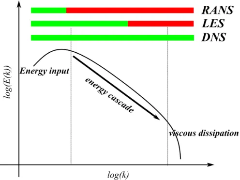
2.4 Energy cascade in turbulent flow. k is the wave-number. The larger k is, the smaller the length scale. The green bars represent the resolved scale ranges and red bars modeled scale range in different simulation strategies. . . 32
2.5 Solution of the model problem 2.8 at different times. ∆x = 0.005. Time is discretized using Forward Euler method. Spatial derivative is approximated using first order upwind finite difference. . . 36
2.6 Variation of wave energy with time for different mesh sizes. . . 37 2.7 The global trail function φi(x) on [0, 1]. The domain is divided into
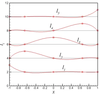
three elements. Inside each element, 4th order Lagrange polynomial is used to construct the piecewise global trail function. . . 41 2.8 4th order Lagrange polynomial on GLL points, liis shifted upwards by
2i. . . 42
2.9 Spectral Element Method solution of the problem 2.9. Six elements, 15th order in each elements. . . 42
2.10 (a) An example of overlapping meshes. (This is just a illustration be-cause there is no need to use two meshes for this simple geometry.) (b) The x velocity of Walsh’s eddy solution at t = 0.04 obtained using the meshes in figure (a) . . . 44 3.1 Variation of Rec, Ur, Utalong the span (Velocities are normalized by U∞). 48
3.2 The first version of the mesh. The domain encloses the whole blade. However, this mesh is too large and lots of elements are wasted because we are only interested in the boundary layer. . . 48 3.3 The mesh for the turbine blade . . . 50 3.4 Boundary layer velocity profile at x/cl = 0.4 y = 25.24m(y/R =
0.63), (a) streamwise velocity (b) radial velocity . . . 52 3.5 Comparison of results obtained by different orders (a) pressure
coeffi-cient along Section8 (y/R = 0.75), normalized by local incoming flow, x coordinate is normalized by local chord length (b) velocity profile at x/cl = 0.5, y = 25.24m(y/R = 0.63) . . . 53
3.6 The spectrum of the circumferential velocity signal (a) x/cl = 0.36,
Section1, Suction side. (b) x/cl= 0.63, Section1, Suction side. . . 53
3.7 Averaged velocity contour (a) 3D blade simulation, circumferential ve-locity on r = 25.24m (b) The same as (a), radial veve-locity (c) 2D simu-lation Ux (c) 2D simulation, spanwise velocity Uy . . . 54
3.8 Comparison of pressure coefficients of 3D simulation, Airfoil simula-tion and wind tunnel measurement . . . 55 3.9 Velocity profile. red-dashed line: 3D rotating blade; black-solid line:
Airfoil (a) Streamwise velocity, Suction side (b) Streamwise velocity, Pressure side (c) Cross-flow velocity, Suction side (d) Cross-flow ve-locity, Pressure side . . . 56 3.10 Coherent structure on suction side. Iso-contour of λ2, colored by
cir-cumferential velocity . (The blade is not to scale) . . . 58 3.11 Skin friction contour. Normalized using U∞ . . . 59
3.12 Close up view of coherent structure on suction side (a) 3D rotating blade simulation (b) Airfoil simulation . . . 60 3.13 Spatio-temporal diagram of velocity signal (a) circumferential velocity
from 3D simulation at y = 25.24m (the sensors are along Section1) (b) Airfoil simulation (the sensors are located along the mid-span section) . 61 3.14 Variation of growth rate of unstable wave with (a) ωr ( Normalized by
1ms. spanwise wave βr number is zero. The arrows mark out the
ob-served ones in the simulations) (b) spanwise wave number βr(ωr = 0.4) 62
3.15 Coherent structure on the pressure side. . . 63 4.1 The expanded blade section (in red) on the z − x plane at y = 0.8.
Parts of the adjacent blades are also plotted. The blue lines are domain boundaries in the circumferential direction. The periodic points pairs have the same z coordinate. . . 67 4.2 The layout of overset overlapping mesh. The outside mesh is in black
and the inside mesh is red.(a)z − x slice of the expanded meshes. (b) x − y slice of the final meshes. . . 68 4.3 Topology of the structured mesh blocks on the blade (the pressure side).
The numbers are the element numbers along the corresponding edges. . 69 4.4 Definition of wall-normal and streamwise directions on the expanded
z − x plane. The geometry non-uniformity in spanwise direction is neglected. . . 70 4.5 First LNS mesh layer on the pressure side of the blade. . . 72 4.6 Uz contour on the expanded z − x slices at y = 0.5 and y = 0.8. The
2D streamlines are based on Uθand Uz, i.e. the radial motion is neglected. 73
4.7 Experiment measurements of Ktand Kqfor different advance ratios J
(from Ref. [65]). The symbols are from current simulations. The order 6 (red) and order 8 (black) results are quite close that they overlap with each other. . . 74 4.8 Estimation of y+ on the suction side. . . 74
4.9 Velocity profiles, the arrows indicate either increasing r or increasing θ. (a) Pressure side, r = 0.8, θ = −7.6◦, 7◦, and 21.2◦ (b) Pressure side, θ = 0◦, r = 0.6, 0.75, and 0.9 (c) Suction side, r = 0.80, θ = 0.0◦, 10.8◦, and 21.5◦(d) Suction side, θ = 0◦, r = 0.65, 0.80, and 0.95 77 4.10 Iso-surface of lambda2 criterion (λ2 = −400) on the suction side,
col-ored by velocity in z direction. . . 78 4.11 Uz contour on the expanded section r = 0.95, which cut through the
center of the small radial aligned structures. The boundary layer is fully attached. The only plausible explanation of the oscillation marked out is T-S waves. . . 78 4.12 Uz contour at different θ locations (the suction side). d is
distance-to-wall. These planes are j − k slices of LNS mesh. (a) θ = 0◦(b) θ = 13◦ (c) θ = 26◦ . . . 79 4.13 Iso-surface of lambda2 criterion on pressure side. . . 81 4.14 Uz contour for different θ locations. (a) θ = −7◦(b) θ = 11◦ (c) θ = 30◦ 82
4.15 2D streamlines and the contour of radial velocity Ur near the trailing
edge on the expanded z − x plane y = 0.45. The radial movement of the streamlines are neglected. Because the blade is not uniform in spanwise, the wall-normal velocity is not exactly zero. As a result, some of the streamlines end on the wall. . . 83 4.16 (a)Streamlines based on the current DNS. They are generated as close
to the wall as possible. (b) Paint streaks from the experiment of [65] . . 84 4.17 Skin friction and streamlines obtained by RANS simulations. From [114]. 85 4.18 αiand αrof stationary cross-flow waves with different βr. The
horizon-tal line marks the αr measured from the DNS. The vertical line marks
the βr measured from the DNS. All the wave-numbers are normalized
using the boundary layer scale 0.01R . . . 88 4.19 Inlet disturbance function (a) a(r) (b) b(d) . . . 89
4.20 LNS simulation (a) Iso-surfaces of Uz0. red: 2 × 10⁻⁵, blue: −2 × 10⁻⁵ (b) Us0 along streamwise direction on the section r = 0.75. s is the local curve length to the inlet on the airfoil. Each red line represents one different wall-normal distance, the envelope of the wave is interpolated from the crests and troughs of the wave. . . 89 4.21 Growth rates along streamwise direction at the section r = 0.75. For
LST, the radial wave-number βr = 3.5, which is the same as the inlet
disturbance of LNS simulation . . . 90 4.22 Iso-contour of perturbed velocity at different time (a) t = 0.128 (b)
t = 0.256(c) t = 0.384(d) t = 0.512 . . . 91 A.1 An example of the Gaussian filter . . . 100 A.2 An example filter kernel function for N = 7 . . . 101 A.3 Smagorinsky length along the channel height, the influence of elements
boundaries can be clearly observed. From [120] . . . 103 A.4 Illustration of flat plate flow set-up (not to scale) . . . 104 A.5 Iso-surface of λ2, colored by distance to wall. (a)DNS (b)LES . . . 105 A.6 Comparison of mean profile (solid lines) and RMS (dashed line) with
that from [122](a) Reθ = 670, (b) Reθ = 1000 . . . 106
A.7 Contour of instantaneous eddy-viscosity from the LES model on a hor-izontal plane. The viscosity is 1/Re = 0.0016. . . 106 A.8 Same as figure 3.5. . . 107 A.9 Same as figure 3.13. . . 107 A.10 (a) Flow structure on the suction side of the center HAWT blade. The
dynamic Smagorinsky model is turned on. (b) The iso-surface of eddy-viscosity obtained by the model. . . 108
R´esum´e en Franc¸ais
Les ´eoliennes `a axe horizontal (HAWT) et les h´elices marines sont deux pplications tr`es ´etudi´es dans le domaine de la recherche en m´ecanique des fluides. Cependant, la transition de couche limite sur celles-ci n’est pas encore enti`erement comprise. Dans cette th`ese, des Simulations Num´eriques Direct sont effectu´ees sur ces deux cas, `a l’aide de supercalculateurs. Le principal l’objectif est d’´etudier l’effet de la rotation sur la transition de couche limite.
Les couches limites des HAWT et des h´elices marines partagent un point commun avec l’´ecoulement de von K´arm´an, qui est cr´e´e par un disque rotatif immerg´e dans un fluide. L’´ecoulement de von K´arm´an peut induire ce que l’on appelle une ’cross flow’ transition. L’objet de la pr´esente ´etude est d’´etudier la possibilit´e d’une transition d’´ecoulement transversal sur les HAWT et les h´elices marines.
Cette ´etude montre que la transition naturelle de couche limite sur les HAWTs et les h´elices marine est induite par des m´ecanismes distinctement diff´erents. Le r´esultat de l’´ecoulement autour d’un pale de HAWT montre que le profil de la couche limite est tr`es proche d’un profil bidimensionel. Sur la pale, la vitesse dans le sens de l’envergure est faible lorsque la couche limite est attach´ee. En cons´equence, la transition naturelle est tr`es similaire au profil 2D et est due aux ondes de Tollmien–Schlichting (T-S).
Sur la pale d’h´elice marine, l’´ecoulement de la couche limite est enti`erement tridi-mensionnel (3D) `a cause des effets combin´es de la rotation et de la g´eom´etrie de la pale. L’instabilit´e et la transition des ’cross-flow’ sont clairement observ´ees. La forme des tourbillons est en bon accord avec la pr´ediction de la th´eorie de la stabilit´e lin´eaire (LST). Bien qu’il ait ´et´e longtemps suppos´e que la ”cross-flow” transition devrait ˆetre importante sur les h´elices, il s’agit de premi`ere observation directe de tels ph´enom`enes `a notre connaissance. Parceque l’h´elice n’a pas de sym´etrie de rotation infinie, notre r´esultat sugg`ere que la couche limite sur les h´elices marines est instable par convection. Cet aspect est diff´erent de l’´ecoulement de von K´arm´an, qui est absolument instable.
Les diff´erences observ´ee sur les ´ecoulements de couche limite sur les HAWTs et les h´elices marines sont probablement caus´ees par leur degr´e de complexit´e g´eom´etrique
variable. La pale de HAWT a un rapport ’aspect tr´es important, par cons´equent, l’´ecoulement transverse n’a pas assez de distance pour se d´evelopper du bord d’attaque au bord de fuite. Au contraire, l’´ecoulement transverse est capable de croˆıtre assez pour conduire `a la transition sur l’h´elice, o`u le rapport d’aspect est petit.
Nous soutenons qu’il est n´ecessaire de travailler dans le r´ef´erentiel rotatif pour ´evaluer l’effet de la rotation. Dans le cas du r´ef´erentiel rotatif, la force centrifuge a une position donn´ee est une constante, tandis que la force de Coriolis d´epend de la vitesse locale. L’amplitude de la vitesse en envergure (cross-flow) est ´etroitement li´ee `a la force centrifuge et `a la force de Coriolis. Par exemple, l’´ecoulement transverse est g´en´eralement le plus forte autour de la s´eparation de couche limite, o`u la force de Coriolis change de direction et agit dans le mˆeme sens que la force centrifuge.
Abstract
The Horizontal Axis Wind Turbines (HAWTs) and marine propellers are two types of important fluid machineries. The boundary layer transition on them is nonetheless not fully understood yet. Equipped with modern cluster computers, Under-resolved Direct Numerical Simulations (UDNS) are performed on both of them in this thesis. The main objective is to study the effect of rotations on the boundary layer transition.
The boundary layers on HAWTs and marine propellers share an apparent common point with von K´arm´an swirling flow, which is created by a rotating disk in the otherwise still fluid. The von K´arm´an swirling flow is the prototype of cross-flow transition. Therefore one focus of the present study is the possibility of the cross-flow transition on HAWTs and marine propellers.
The present study shows that the natural boundary layer transitions on the HAWT and the marine propeller are induced by distinctively different mechanisms. The numer-ical result of a HAWT blade shows that the boundary layer profile on it is very close to the 2-Dimensional (2D) airfoil flow. On the blade, the velocity in spanwise direction is small in the attached boundary layer. As a result, the natural transition on HAWT blade is very similar to the 2D airfoil flow and is due to Tollmien–Schlichting (T-S) waves.
On the marine propeller blade, the boundary layer flow is fully 3-Dimensional (3D) due to the rotation. The cross-flow instability and transition are clearly observed. The shapes of the cross-flow vortices are in good agreement with the prediction of Linear Stability Theory (LST). Although it has been long assumed that cross-flow transition should be important for propellers, this is the first direct observation of such phenomena as far as we know. Because the propeller does not have infinite rotational symmetry, our result suggests the boundary layer on the marine propeller is convectively unstable. This is different with the von K´arm´an boundary layer flow, which is absolutely unstable.
The difference in boundary layer flows and therefore transitions between the HAWT and the marine propeller is likely caused by their shapes. The HAWT blade has a very large aspect ratio, consequently, the cross-flow does not have enough distance to develop from the leading edge to the trailing edge. On the contrary, the cross-flow
velocity is able to grow large enough to lead flow transition on the propeller, where the aspect ratio is small.
We also argue that it is necessary to work in the rotating reference frame in order to evaluate the effect of rotations. In the rotating reference frame, the centrifugal force at one position is a constant, while the Coriolis force depends on the local velocity. The magnitude of the spanwise (cross-flow) velocity is closely related to the relative strength of centrifugal and Coriolis forces. For example, cross-flow is usually the largest around separation bubbles, where Coriolis force changes its direction and acts in the same direction as centrifugal force.
Acknowledgements i
List of Figures iii
Abstract xi
1 Background and Introduction 1
1.1 Background . . . 1
1.1.1 Motivation of the present work . . . 2
1.2 Aerodynamics of 2-Dimensional Airfoil . . . 3
1.3 The boundary layer and its transition . . . 4
1.3.1 The boundary layer . . . 4
1.3.2 The laminar-turbulent transition . . . 5
1.3.3 T-S wave instability . . . 6
1.3.4 Flow separation induced transition . . . 7
1.3.5 Cross-flow transition . . . 9
1.3.6 Others . . . 11
1.4 Transition on the 2D airfoil . . . 11
1.5 The rotating disk flow . . . 12
1.5.1 Cross-flow velocity . . . 12
1.5.2 Its transition . . . 16
1.5.3 Implication . . . 17
1.6.1 HAWTs blades boundary layer . . . 18
1.6.2 Cavitation and marine propeller boundary layer . . . 21
1.7 Summary . . . 25
2 Methodology 27 2.1 Hydrodynamic instability . . . 27
2.1.1 The Linearized NS equations . . . 28
2.1.2 Linear Stability Theory . . . 29
2.1.3 Further notes on LST . . . 31
2.2 Comparison of different simulation strategies for transitional flows . . . 32
2.2.1 RANS . . . 33
2.2.2 LES . . . 34
2.2.3 DNS . . . 36
2.2.4 Choice of the numerical method . . . 37
2.3 Spectral Element Method . . . 38
2.3.1 Spectral Method . . . 38
2.3.2 Spectral Element Method . . . 39
2.3.3 Nek5000 . . . 43
2.3.4 NS equations in the rotating reference frame . . . 45
2.3.5 IDRIS . . . 46
2.4 Summary . . . 46
3 Rotating HAWT blade 47 3.1 Set-ups of the simulations . . . 47
3.1.1 The HAWT blade . . . 47
3.1.2 The meshes and boundary conditions . . . 49
3.1.3 The 2D airfoil simulation . . . 50
3.2 Results . . . 50
3.2.1 The influence of BCs at two ends . . . 51
3.2.3 Flow fields . . . 54
3.2.4 Boundary layer instability and transition . . . 57
3.3 Summary . . . 61
4 Marine propeller 65 4.1 Methodology . . . 65
4.1.1 Blade geometry and parameters . . . 65
4.1.2 Overlapping overset meshes . . . 67
4.1.3 Definition of local flow directions . . . 69
4.1.4 LNS simulation mesh . . . 71
4.2 Results . . . 72
4.2.1 Overlapping overset meshes . . . 72
4.2.2 Mesh convergence and velocity profiles . . . 73
4.2.3 Laminar-turbulent transition on the blade . . . 76
4.2.4 Separation-induced transition and the influence of rotation . . . 82
4.2.5 Flow transition’s influence on the surface streamlines . . . 84
4.3 Stability Analysis . . . 86
4.3.1 Linear Stability Analysis . . . 86
4.3.2 Linearized Navier-Stokes simulation . . . 87
4.3.3 Convective/absolute nature of the instability . . . 90
4.4 Summary . . . 93
5 Conclusion and Perspectives 95 5.1 Conclusion . . . 95
5.2 Perspectives . . . 96
A The Explicit LES model in the Nek5000 99 A.1 Filtering . . . 100
A.2 Averaging of the eddy viscosity . . . 102
A.3 Test cases . . . 103
A.3.2 The wind turbine blade . . . 106
Background and Introduction
1.1
Background
As a source of renewable energy, the installation capacity of wind turbines has been in-creasing steadily around the world. It is projected that this trend would last at least for the foreseeable future. What’s more, the recent development of offshore wind turbines offers a new promising possibility. As one of the fundamental problems, the aerody-namic of wind turbines and wind farms has attracted many researchers.
As indicates by its name, one of the many research fields of the LHEEA (Laboratory in Hydrodynamics, Energetics and Atmospheric Environment) in ECN ( ´Ecole Centrale de Nantes) is the wind energy. The specific topics under active studies in the lab include the aerodynamic of blade sections [1, 2], turbine wakes [3], as well as floating wind turbines etc.
Another broad topic in the LHEEA lab is the naval engineering. The research areas include cavitation of marine propellers [4], development of composite hydrofoils [5], and numerical methods for hydrodynamic [6, 7] etc.
HAWTs harvest energy from the wind. The torque that drives motors is from the lift force on airfoil sections of the turbine blades [8]. Whereas marine propellers exert energy to the surrounding fluid. The propulsion is also from the lift force on sections [9]. Although the HAWTs and marine propellers have quite different geometries and
working conditions, they are both based on the aerodynamic of 2D airfoils. Except this, there is another apparent similarity, i.e. they both rotates.
(a)
(b)
Figure 1.1: (a) NM80 wind turbine in the DanAero MW project. (b) A marine propeller, from Wikipedia.
1.1.1
Motivation of the present work
The fact that both HAWTs and marine propellers rotate during operations makes them bear a resemblance to one of the most classic problems in fluid dynamic, which is the laminar-turbulent transition of the rotating disk boundary layer.
The most notable feature of the rotating disk boundary layer is the 3D effect on the boundary layer due to the rotation. This gives rise to a totally different transition mech-anism from 2D boundary layers, namely the cross-flow transition [10]. However, most studies on HAWTs and marine propellers’ boundary layer transition are based on 2D airfoils. To get better understanding of the process on HAWTs and marine propellers, it is necessary to quantify the effect of rotations.
In the rest of this chapter, we will firstly give a brief description of the aerodynamics of 2D airfoils. Then the laminar-turbulent transition of boundary layer is introduced, followed by the description of possible transition scenarios related to the present study.
We then revisit the rotating disk flow and its transition. The rise of cross-flow inside boundary layer is explained. We re-state the similarity between the rotating disk flow and HWATs and marine propellers. At last, the state-of-the-art about the boundary layer transition on rotating blades is reviewed.
1.2
Aerodynamics of 2-Dimensional Airfoil
The airfoil is the basis of many practical fluid machinery including HAWTs, propellers, and airplane wings et al. It is a lift generating structure. Figure 1.2 gives an illustration of the flow around a typical 2D airfoil. When the flow passes around the airfoil, there usually exists a pressure difference between the two sides of the airfoil (the side with large pressure is usually referred to as the pressure side, and the one with smaller pres-sure is referred to as the suction side). This prespres-sure difference is the main source of the force on the airfoil.
Figure 1.2: Flow around a 2D airfoil. The incoming flow is in x direction.
The force component parallel to the incoming flow is the drag. The component perpendicular to the incoming flow is the lift. The magnitude of the lift depends on many parameters and is measured by lift coefficient Cl. For a given airfoil, one of the
most important parameter determining Cl is Angle of Attack (AoA).
AoA measures the angle between the incoming flow direction and the direction of airfoil’s chord, which is the line connecting the leading edge and the trailing edge of the airfoil. When AoA is small, lift coefficient Cl roughly increases linearly with
AoA as predicted by lifting-line theory. However, if AoA further increases, the Cl
would decrease rapidly after Clhaving reached maximum. At the same time, the drag
increases as well. This phenomenon is called ’stall’.
Stall is generally related to massive flow separations on the airfoil [11, 12]. Pressure gradients always present along the airfoil chord. The adversary pressure gradient (where the downstream pressure is larger than upstream pressure) is inevitable due to the nature of airfoils. The adversary pressure gradient would decelerate the flow. When the inertial force is not able to overcome the adversary pressure gradient, the attached boundary layer flow could separate for the wall surface.
When AoA is small, the flow separation does not exist or is very weak. The flow usually reattaches after separations, which is usually close to the trailing edge. As AoA and the adversary pressure gradient increase, the separation points moves upstream on the airfoil. Under stall conditions, massive flow separations appear close to leading edge [12] and the flow does not reattach. The effective shape of the airfoil is profoundly changed and its aerodynamic performance deteriorates.
1.3
The boundary layer and its transition
1.3.1
The boundary layer
On the airfoil surface, the flow velocity decelerates to zero due to the non-slip boundary condition. Very close the airfoil wall, there exists a thin layer of fluid, through which the outside inviscid flow velocity decreases to zero on the wall. This fluid layer is referred to as ’boundary layer’ and is firstly discovered by Prandtl [13]. The importance of the boundary layer could not be emphasized too much.
Figure 1.3 shows the Blasius profile, which describes the boundary layer formed by flow over a flat plate. It is a self-similar solution in that the velocity profiles at different streamwise locations x is the same after being normalized. The boundary layer thickness of Blasius solution increases along streamwise direction according to δx ∝
√
self-Figure 1.3: Blasius boundary layer on a flat plate.
similar and can be described by the Falkner-Skan solution [13]. Inside the boundary layer, the large velocity gradient in wall-normal direction makes the viscous force non-negligible.
The boundary layer around airfoil is usually not self-similar. However, many con-cepts from Blasius solution can be applied to airfoil boundary layer. For example, they both develop from the leading edge toward downstream. The same technique is often used in the derivation and solving of the boundary layer equation for airfoil. What’s more, the transition on airfoils is very much similar to flat plate when the boundary layer is attached.
1.3.2
The laminar-turbulent transition
The famous Reynolds’ experiment [14] on the pipe flow shows that there are two dif-ferent flow states depends on a parameter which is now called Reynolds number (Re). When Re is small, the dye streaks are aligned with each other and the flow is laminar. When Re is large, the flow become chaotic and turbulent.
The laminar-turbulent transition has many implications on the aerodynamic perfor-mances of the bodies. It affects flow separation, increases drags, and introduces fluc-tuating loads etc. The transition process of boundary layer flow is quite complex and depends on many factors. Figure 1.4 summaries the main routes through which a lami-nar boundary layer could become turbulent. In short, if the flow is unstable to external
Figure 1.4: Paths to transition with increasing environmental disturbances. In this the-sis, we only consider the path A in the figure. From [15]
disturbance, the disturbance would increase its magnitude and eventually leads to flow transition.
In this thesis, only the natural transition is considered (Path A in figure 1.4). Al-though natural transitions are more common when the environmental disturbances are small, a good understanding of them is important to predict the boundary layer’s re-sponses to large disturbances. In the following subsections, several natural transition modes pertain to airfoil boundary layers are described briefly.
1.3.3
T-S wave instability
The Blasius boundary layer is subjected to the Tollmien-Schlichting (T-S) instability, which is firstly studied theoretically by Tollmien and Schlichting around the late 1920s. It was confirmed by the experiments of Schubauer and Skramstad [17, 18]. Figure 1.5 shows the different stages in the T-S wave transition. Near the leading edge, where the Reynolds number Reδ is small, the flow is laminar and stable. As the boundary layer
thickness increases downstream, the local Reδ increases as well. The laminar flow
Figure 1.5: Top view and side view of the T-S wave transition on the flat plate. From [16]
form 2D T-S waves through the ’receptivity’ process. The amplitude of the T-S wave grows exponentially along the streamwise direction. When the amplitude of the distur-bance wave reaches around 2% ∼ 10% of the boundary layer edge velocity, nonlinear interactions between different T-S waves become significant. The new flow field, which is greatly modulated by the 2D unstable wave, becomes unstable to 3D disturbance. When the 3D disturbance becomes large, the flow usually exhibits Λ structures. The 3D flow structure itself is quite unstable and would quickly breakdown to smaller struc-tures. The transition process finishes and the flow becomes fully turbulent.
1.3.4
Flow separation induced transition
The Laminar Separation Bubble (LSB) is commonly seen on the suction side of airfoils. Figure 1.6 depicts the flow structures around a 2D LSB. The adversary pressure gradient in stream-wise makes the initially wall-attached streamlines to separate from the wall. A recirculation zone appears near the wall with part of the fluid moves reversely. After the boundary layer transition to turbulent, the streamlines reattaches.
Depending on many factors such as the geometry of airfoil, Re, AoA, and inflow conditions [20, 21], LSBs have different shapes. However, they are generally quite
Figure 1.6: Flow structures around a typical 2D separation bubble. From [19]
Figure 1.7: LSB induced transition on a flat plate. The flow separation is caused by ad-versary pressure gradient. The contour is based on the normalized streamwise velocity.
unstable when Re is large. The wall-normal velocity profile of LSB usually has an inflectional point, making it unstable according to inviscid stability theory.
When the separation bubble is small, the unstable T-S wave, which appears in the upstream attached boundary layer, can go through the LSB. In Ref. [22], the growth rate of the T-S wave in separation region obtained from DNS (Direct Numerical Simulation) agrees quite well that from LST. Inflectional instability can also happen due to the upstream disturbance [23]. However, this instability is convectively unstable in nature.
mech-anism would dominate the transition process. The boundary layer velocity profile with large reverse flow is similar to a mixing layer, where rapid flow transition can be ob-served due to Kelvin-Helmholtz (K-H) instability. Similar transition processes to K-H instability are often observed around the LSB. The primary stability results in 2D shed-ding vortices. As the shedshed-ding vortices being convected to downstream, secondary instability occurs[24]. The flow becomes rapidly turbulent. Figure 1.7 shows the struc-tures in a LSB induced transition, where the rollers are clearly visible.
Similar to the K-H instability, LSB is absolute unstable when the reverse flow is large. As a result, the LBS always exhibit unsteadiness. Pauley et al. [25] use the Stroulhal number based on the boundary-layer momentum thickness at separation and the local free-stream velocity to quantify the shedding frequency, which is in agreement with the prediction of linear inviscid stability theory.
It should be noted that there is no universal criterion to determine whether the LSB is large or small. Generally speaking the flow is absolute unstable only when the reverse flow is as large as 12% − 20% of the boundary layer edge velocity [26, 27]. The inter-actions between the viscous instability and the inflectional instability are also reported in the literatures (for example [28]).
1.3.5
Cross-flow transition
So far, we have been talking about 2D boundary layer. i.e. the flow is homogeneous in one direction (usually spanwise) and the fluid does not move along that direction. How-ever, 3D boundary layer, where there is no homogeneous direction, is quite common in practical engineering flows.
Figure 1.8 shows the typical flow structure inside a 3D boundary layer. Inside the boundary layer, there is a velocity component which is perpendicular to the inviscid flow direction. This velocity profile is refereed to as ’cross-flow’.
Because cross-flow is zero on the wall and outside the boundary layer, its profile usually has an inflectional point, which makes it unstable according to the Rayleigh theorem. The cross-flow transition can be observed in many typically 3D flows, e.g. the
Figure 1.8: 3D boundary layer flow structure. From [15]. yt is the local wall-normal
direction. xt is the local streamwise direction and zt is perpendicular to xt and yt.
Outside boundary layer, the velocity is totally in streamwise direction. However, there is a velocity component in ztdirection inside the boundary layer.
Figure 1.9: Cross-flow vortices and flow transition (iso-surface of λ2). The inviscid flow is roughly in x direction. From [31]
.
rotating disk [29], swept wings [15], and the yawed cone [30] etc.
Figure 1.9 shows the process of cross-flow transition. Similar to the T-S wave tran-sition, the whole process can be roughly divided into linear, nonlinear (saturation), and breakdown stages. The small disturbance, which usually form a wave pattern in the cross-flow direction, firstly grows exponentially in the linear stage. As goes to down-stream, the wave develops into streamwise vortices with larger amplitude. Both sta-tionary and traveling cross-flow vortices can exist. When their amplitudes are around 1% ∼ 10% of the streamwise inviscid velocities, nonlinearity comes into effect. The vortices grow with smaller growth rates and eventually saturate. The saturated cross-flow vortices can maintain a rather long distance. Their cross-flow structures are usually referred to as ”half mushroom” in contrast to the ”mushroom” structures observed in G¨ortler instability.
(a) (b)
Figure 1.10: (a) The mushroom-like structure in G¨ortler instability. From [32]. (b) The half mushroom structure in cross-flow instability. From [33].
The saturated cross-flow vortices are subjected to the secondary instability. In this stage, the vortices are unstable with respect to high-frequency oscillations. With the growth of secondary instability, the flow quickly becomes turbulent.
1.3.6
Others
Many other unstable modes also exist depending on the flow configurations. For exam-ple, along concave walls, G¨ortler instability often appears in the boundary layer. The flow along the leading edge of a swept wing is subjected to so-called ’leading edge con-tamination’. Roughness elements on the wall can also lead to boundary layer transition.
1.4
Transition on the 2D airfoil
On 2D airfoil without swept or where the blade spanwise variation is small, the natural transition of the boundary layer can be either triggered by T-S wave or flow separation. When the Reynolds number is large, the boundary layer close to the leading edge would be unstable to T-S wave [34, 35]. The T-S wave on the airfoil is very much similar to the flat plate case describe above. However, there is usually a pressure gradient along the streamwise direction on the airfoil. Similar to the Falkner-Skan boundary layer [36], the adversary pressure gradient has a dis-stabilizing effect whereas the favorable pressure gradient makes the boundary layer be more stable.
When the chord Reynolds number is small (for example, the unmanned aerial ve-hicles), the laminar boundary layer can maintain a long distance on the airfoil. In that case, the boundary layer transition is usually triggered by the LSB, which appears when
Figure 1.11: Illustration of streamlines in inviscid region and in boundary layer on a rotating disk. Because the wall-normal velocity, which is parallel to the angular velocity vector, does not affect the direction and magnitude of the forces, therefore it is neglected in plotting these streamlines
the local adversary pressure gradient is large [2].
1.5
The rotating disk flow
1.5.1
Cross-flow velocity
The laminar rotating disk flow has an exact self-similar solution of the Navier-Stokes (NS) equations, which is first discovered by von K´arm´an [37]. It can be classified into a family of NS solutions, where rotations play an important role [38, 39]. The essential feature of von K´arm´an flow is the appearance of cross-flow velocity inside boundary layer, which can be explained by the relationship between centrifugal and Coriolis forces in the rotating reference frame.
Let’s consider the flow on a rotating disk in figure 1.11, which rotates with an an-gular velocity ω = (0, 0, ωz). It is natural to work under the rotating reference frame in
which the disk is stationary. Because rotating reference frames are non-inertial frames, two additional fictitious forces arise. The centrifugal force −ω × (r × ω) on a fluid parcel at r = (r, θ, z) (r, θ, z are radius, angle, and depth coordinates respectively in the cylindrical system, which is in the rotating reference frame) is (rωz2, 0, 0). And the Coriolis force −2ω × U on it would be (−2uθωz, 2urωz, 0), where U = (ur, uθ, uz) is
In the rotating reference frame, we can treat the fictitious forces like real forces, and pretend we are in an inertial frame [40]. For a fluid parcel far away from the disk, it is not affected by the presence of the disk (the wall-normal velocity induced by the disk is neglected, which would not change the analysis) and does circular motion with radius r and uθ = rωz. The centripetal force needed for this circular motion is (−rω2z, 0, 0),
which is exactly the combination of the corresponding centrifugal force and Coriolis force.
For a fluid parcel at the same r but inside the boundary layer, its circumferential velocity uθ is smaller than rωz because of non-slip boundary condition. Therefore,
the Coriolis force, which depends on the velocity, is smaller than the inviscid case. However, the centrifugal velocity force, which depends only on r, is the same as the inviscid case. As a result, the combination of the centrifugal force and Coriolis force is no longer large enough to keep the fluid parcel doing circular motion with radius r, but with a larger radius. This means that a radial velocity appears inside the boundary layer. The cross-flow velocity profile introduces an inward viscous stress in radial di-rection, which partially counteract the outward motion to the extent that an equilibrium is reached.
Figure 1.12 summaries the above process. In short, the radial (cross-flow) veloc-ity can be seen as a secondary flow induced by the primary flow in circumferential direction. Later we will see that the process illustrated in the figure can explain the more complex phenomena on rotating blade boundary layer. For example, when flow separates, the Coriolis force changes its direction and acts in the same direction as cen-trifugal force. On the other hand, because the separation bubble is usually thicker than the attached boundary layer, the viscous force is small. These two factors would result a large radial flow around separation regions.
Figure 1.13 plots the velocity profiles of von K´arm´an solution from [10]. The cir-cumferential velocity is similar to the Blasius boundary layer. However, the radial ve-locity inside boundary layer is not zero as explained above. Because the fluid is pumped outwards near the wall, there is a wall-normal velocity so the continuity equation is
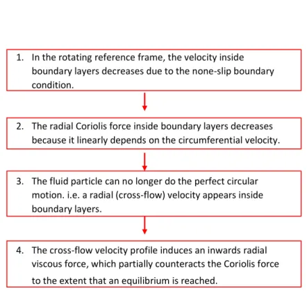
sat-1. In the rotating reference frame, the velocity inside boundary layers decreases due to the none-slip boundary condition.
2. The radial Coriolis force inside boundary layers decreases because it linearly depends on the circumferential velocity.
3. The fluid particle can no longer do the perfect circular motion. i.e. a radial (cross-flow) velocity appears inside boundary layers.
4. The cross-flow velocity profile induces an inwards radial viscous force, which partially counteracts the Coriolis force to the extent that an equilibrium is reached.
Figure 1.12: The arise of the cross-flow velocity in the rotating disk boundary layer.
Figure 1.14: The flow inside a teacup, which is an example of B¨odewadt layer. Here the cross-flow velocity is towards the rotating axis. From [41]
isfied. It should also be noted that the Re in the rotating disk flow is usually defined as rpω/ν, where ν is the kinematic viscosity.
Another example of the rotating flow system is the B¨odewadt layer, where the disk is at rest while the inviscid flow rotates. It can be analyzed in the rotating reference frame similarly. Like the von K´arm´an flow, there is a cross-flow velocity close to the disk. However, the cross-flow velocity in B¨odewadt layer is towards the rotating axis. A daily example is the flow inside a teacup. After stirring, the tea-leaf at the cup bottom would alway come to the center.
1.5.2
Its transition
(a)
(b)
Figure 1.15: (a) Boundary layer transition on the rotating disk. The spirals are cross-flow vortices. (b) Close-up view of the cross-cross-flow vortices. The high-frequency oscil-lations due to secondary instability can be clearly seen. From [42].
The cross-flow profile is unstable as it has an inflectional point. Figure 1.15 shows the experimental visualization of the cross-flow transition on the rotating disk, which is similar to the description in 1.3.4. Around the center of the disk, the flow is laminar as the local Reynolds number is small. At larger radius, the spiral vortices are unstable cross-flow waves, which grow outwards and lead to the transition.
The cross-flow instability has received much attention because of its importance in modern airliner swept wings [15]. As a prototype for cross-flow transition, the rotating disk boundary layer has been under extensive theoretical, experimental, and numerical studies for its geometry simplicity. In the experiment of Gregory et al. [43] around 30 stationary spiral vortices were observed on the disk. The vortices propagate in the direction predicted by the inviscid stability theory. Malik et al. [44] showed that the
Coriolis and curvature terms, which have a stabilizing effect, need to be included in linear stability analysis. The critical Reynolds’ Recnumber obtained by Linear Stability
Theory (LST) is around 287, which is in agreement with their experiment (Rec = 294)
and the experiment (Rec = 297) of Kobayashi [42]. In the two important works of
Lingwood [10, 45], the author found that the boundary layer on the rotating disk is absolutely unstable when Re is larger than 510. This value corresponds well with the turbulence onset Re observed in several experiments. However, later it is shown that the cross-flow instability are only convective unstable in Falkner-Skan-Cooke (FSC) flows and swept wing boundary layer [29, 46]. The global instability of rotating disks has also been discussed in many literatures[47].
1.5.3
Implication
As mentioned earlier, both HAWTs and marine propellers rotate during operation. As a result, the same reasoning in figure 1.12 can be readily applied. There should be a cross-flow velocity in their boundary layers. Therefore, a natural question to ask is whether cross-flow instability and transition can be observed on HAWTs and marine propeller blades.
1.6
HAWTs and marine propellers
The boundary layer’s state could have a big implication on the aerodynamic of the bodies. A well-know example is the dimples on golf balls, which prompt the boundary layer transition. The turbulent boundary layer is usually harder to separate from the wall. The drag is therefore smaller and the golf ball can fly farther.
A good knowledge of the transition process is needed to model it in numerical sim-ulations, which are widely used to predict and optimize the performance of turbines or propellers. Much effort has been done to understand the transition on rotating blades in the past decades.
1.6.1
HAWTs blades boundary layer
Effect of the rotation
HAWT blades consist of a series of 2D airfoil sections with different thicknesses, chord lengths, and twist angles. In the design and optimization of HAWTs, Blade Element Theory (BET) is widely used. After dividing the blade into sections (or elements) in the spanwise direction, BET assumes that the flow around each section is locally 2-dimensional. The lift and drag forces for each section can be obtained from momentum theory or calculated from 2D potential flow code such as XFOIL[48]. The total torque of the blade can be then obtained by summing local sections’ performance together[8, 49].
Nonetheless, the flow around the HAWT blade is not strictly 2D. As early as 1945, Himmelskamp [50] observed that the lift coefficient for the rotating blade is increased compared with the non-rotating case, and the stall is postponed. This phenomenon is referred to as rotational augmentation in the later literature. Fogarty[51] solved the boundary-layer equations for rotating blade and found that the effect of rotation is small, which contradicts with engineers’ impression. He suggests one of possible reasons might be that his analysis is only valid for attached flow region. McCroskey’s flow visualization of rotating blade shows that the boundary layer transition on rotating blade resembles non-rotating blade, but there is a significant outward radial velocity in laminar separation bubble and in trailing-edge separated flow [52]. Snel[53] performed a scale magnitude analysis for rotating blade boundary layer equations, where he con-sidered flow separation. His results show an improved Cl prediction compared to 2D
calculation. Corten[54] pointed out that the boundary layer assumption in Snel’s anal-ysis is not necessary for separation regions. He also shows that the separated flow will move in outward radial direction due to centrifugal force.
Nowadays, it is well recognized that rotational augmentation is closely related to the large spanwise velocities in separation regions. On the one hand, the radial velocity pumpfluid from separation region to spanwise direction, leading to volume reduction of separation bubble[55]. On the other hand, the radial velocity induces a streamwise
Coriolis force, which partially counteracts the adverse pressure gradient[56].
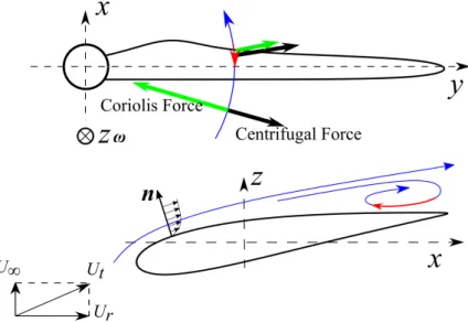
Figure 1.16: Inside the separation bubble, streamwise velocity changes its direction (red arrow), which causes the Coriolis force (green arrow) acts in the same direction as the centrifugal force (black arrow).
In section 1.5, we pointed out the similarity between the boundary layer flows on HAWT blades and on the rotating disk. Here we argue that the radial velocities in sepa-ration regions of HAWT blades can be analyzed similarly. Here we repeat the argument. In figure 1.16 a blade is rotating in the plane (x, y), i.e., the angular velocity ω of the rotating reference frame fixed to the blade is (0, 0, ωz). Considering a fluid parcel at
r = (r, θ, z) (r, θ, z are radius, angle, and depth in the cylindrical coordinate system respectively), its velocity relative to the rotating reference frame U is (ur, uθ, uz). The
centrifugal force −ω × (ω × r) on this fluid parcel would be (rω2z, 0, 0) (in local radial, circumferential, and depth directions respectively). And the Coriolis force −2ω × U on it would be (−2uθωz, 2urωz, 0).
Far away from the blade, the fluid parcel experience circular motion with uθ = rωz.
The centripetal force needed for this circular motion is (−rω2
z, 0, 0), which is exactly the
combination of centrifugal and Coriolis forces. When flow detaches, the circumferential velocity decreases and reverses its direction. As a result, Coriolis force changes its direction and acts in the same direction as centrifugal force, which results in large radial velocity ur.
boundary layer as well. The argument on the rotating disk flow applies to HAWT blades without any changes (please refer to section 1.5). Indeed, this radial velocity was ob-served in [57], where the boundary layer equations on a rotating blade was solved.
Boundary layer transition on rotating blades
Figure 1.17: Transition location on the center of a HAWT blade (where there is a glove). Visualized using thermal images. The bright color is laminar flow whereas dark color is turbulent. (a) Start-up stage. (b) Operating. From [58]
The laminar-turbulent transition on HAWTs is drawing increasing attention. It not only affects aerodynamic characteristics like lift and drag but also generates load fluctu-ations, which might decrease the rotor life. Much endeavor has been made to understand the flow transition on rotating blade.
Bosschers et al. [57] solved the boundary layer equation on a rotating blade and observed a cross-flow velocity component. They pointed out that laminar-turbulent transition on a rotating blade might occur due to cross-flow. Heister’s [59] study of he-licopter rotor shows there coexist multiple transition scenarios, including bypass transi-tion, leading edge contaminatransi-tion, cross-flow transitransi-tion, and T-S wave. Hernandez [60] performed LST analysis on rotating flat plate boundary layers to study the transition on HAWT. Although there is a cross-flow component in the base flow, his analysis is only restricted to T-S waves. Weiss [61] measured the boundary layer transition on rotating blades by temperature-sensitive paint. He also performed LST analysis and found that the critical transition N-factor is around 8.4.
Figure 1.18: An example of transition location (red line) derived from pressure fluctua-tions, which varies with time. From the DanAero MW project. For the meaning of the symbols in the figure, please refer to [62]
Due to the rotation and their large scale, it is very challenging to detect and measure the unstable waves HAWT blades in similarly to the flat plate. However, the transition locations on full-scale HAWTs are obtained using different experimental techniques.
In Reichstein et al. [58], the thermo-graphic imaging was used as a non-intrusive method for detecting flow transition on a MW wind turbine. The transition location from thermo-graphic imaging is in good agreement with results from microphones and transitional CFD simulations. Figure 1.17 is taken from [58]. It can be seen that when the wind turbine is in regular operation mode, the transition appears quite near the leading edge (x/c = 0.05).
In the DanAero MW projects[63, 64], the transition location on a MW turbine is derived from surface pressure fluctuations measured by microphones. The transition location on the full scale turbine blade is advanced as compared to wind tunnel exper-iments. This difference of transition locations is caused by different characteristics of incoming turbulence in wind tunnel and field measurements.
1.6.2
Cavitation and marine propeller boundary layer
The marine propeller is another important type of flow machinery. Similar to HAWT blades, propeller blades are based on the hydrodynamic of 2D blade. However, pro-peller sections are defined on a series of concentric cylindrical surfaces as shown in
Figure 1.19: The Propeller C from Kuiper [65]. The green surface is one of the cylin-drical surfaces on which the blade sections are defined.
figure 1.19. After expanding the cylindrical surfaces, the sections on them are simply 2D airfoils. The lift force on the expanded 2D sections has two components. It is the component parallel to the shaft axis that provides the propulsion.
The boundary layer transition
The boundary layer around marine propellers is a typical 3-Dimensional (3D) flow due to the geometries and rotations. Transitional flow can be often observed on the model testing propellers.
Similar to the HAWTs, transition locations on propeller blades can be obtained ex-perimentally. In the classic work of Kuiper [66], he shows that although the exact transition location on propeller blades depends on a number of factors, the flow regimes can be generally divided into laminar and turbulent regions according to the direction of paint streaks. In the laminar flow region, the paint streaks point outwards towards the tip, whereas they are aligned to the circumferential direction in the turbulent region. This streamline pattern difference is still the most commonly-used criteria to distinguish the flow status in marine propeller experiments [67, 68].
Using oil-film interferometry, Sch¨ulein et al. [69] obtained the friction coefficient on a whole blade of a high-speed aeronautic propeller. Some fine flow structures, not only in the attached flow but also in the separation bubble, are also clearly visualized in
their paper. However, these works are more focused on transition locations on propeller blades instead of the transition process itself.
There are also numerous of CFD studies about the transition on propeller blade. At present, almost all those studies rely on the RANS, where transition models are usually used to capture the boundary layer transition. Transition models in the RANS usually include empirical correlations and their effectiveness depend on the transition scenarios [70, 71]. Therefore, the understanding of possible transition mechanisms is vital for modeling the transition problem. One of the most popular transition models is γ − Reθ model developed by Menter et al. [72]. Bhattacharyya et al. [68] shows that
the inclusion of γ − Reθ model results a better agreement with experimental paint test
in terms of flow patterns on the propeller. Pawar and Brizzolara [73] show that γ − Reθ
is able to correctly predict the complex flow phenomena on propellers like leading edge separation. However, the inlet condition need to be tuned RANS in order to get a better agreement with experiment. In the Moran-Guerrero et al.[74], they investigated the boundary layer transition on a propeller using γ − Reθ that is able to take cross-flow
into account. They show that the addition of cross-flow terms in the γ − Reθmodel can
promote the transition onset and result a larger turbulent region.
Interaction with cavitation
The cavitation is perhaps the most important and challenging problem on ship pro-pellers. As mentioned above, propellers work based on the pressure difference between the two sides of the blades. When the pressure on the suction side decreases too much locally, the fluid could become vapor rapidly. When the bubble ( or cavity ) filled with vapor is convected to downstream where the ambient pressure is large, it collapses. Dur-ing the implosion, there is usually a high speed water jet which can reach supersonic speed. If the water jet hits the propeller, it exerts a considerable force on the body. Be-cause the cavitation can generate numerous bubble, it is a main Be-cause of propeller wear and failure.
Figure 1.20: Illustration of the suction side Cp, flow structure and the cavitation on
hydrofoil sections.
When the AoA is large, a low pressure region forms near the leading edge. If the pressure is small enough, a large, quasi-steady cavity of vapor could appear. On a whole blade, this forms so-called sheet cavitation as shown in the figure 1.21a. If the pressure is small locally and there is nuclei, bubble cavitation would appear (1.21b).
(a) (b)
Figure 1.21: (a)Sheet cavitation (b) Bubble cavitation. From [75]
In the transition flow region, the pressure fluctuates at a significant magnitude. Pre-vious studies show that the cavitation might occur either at the location of minimum Cp
or at the transition region [76]. The fluctuation in the laminar separation bubble might affect the inception of sheet cavitation [77, 78, 79] whereas the turbulent spot during
transition can affect the bubble cavitation [75].
1.7
Summary
At the beginning of this chapter, we introduced some basic fluid dynamic concepts such as airfoil aerodynamics, boundary layers and the laminar-turbulent transition. Then we explained the origin of cross-flow on the rotating disk and its transition.
After having pointed out the similarity between the rotating disk and HAWTs and marine propellers, we reviewed the related works on rotating blades’ boundary layer. Although many works has been done, they are more focused on the transition location on HAWT and propeller blades. Little is known about the transition process itself on rotating blades.
Indeed, the complex operating conditions, twisted geometries and unsteadiness make the accurate measurements of the boundary layer profile and transition by experiments to be very difficult. On the other hand, CFD offers a feasible approach, which can get the full information of the flow fields. To the best of our knowledge, there is no numer-ical simulation which fully resolve the laminar-turbulent transition on rotating HAWT or propeller blades. This work aims partially fill this gap.
Methodology
In this chapter, we will first present the stability theory. Then we offer a description of Spectral Element Method, which is the main numerical tool used in this thesis. How-ever, both subjects are so developed that it is impossible to give an extensive explana-tion. Therefore, we will focus on the basic concepts and terminology. References are given as much as possible.
2.1
Hydrodynamic instability
Stability theory studies the response of a system when it is disturbed. The toy in figure 2.1 together with a horizontal plane define a stable system. The base state of the toy is simply stationary. Any disturbance added to it would decay due to frictions and the system would finally return to the base state. It likes the G¨omb¨oc which would always return to the same position.
The laminar-turbulent transition is usually accompanied by the amplification of small disturbances. The hydrodynamic instability theory attempts studies the evolution of small disturbances in the laminar flow. If the disturbance increases in its amplitude, the laminar base flow is said to be unstable and could transition to turbulence. The development history of the linear instability theory can be found in the monograph of Drazin and Reid [18].
(a) (b)
Figure 2.1: (a) A traditional Chinese roly-poly toy (A-person-won’t-fall). It is an ex-ample of a stable system. From taobao.com (b) The G¨omb¨oc, which is a homogeneous body having just one stable and one unstable point of equilibrium. From Wikipedia.
2.1.1
The Linearized NS equations
The low-speed motion of Newtonian fluid is governed by the incompressible Navier-Stokes equations, which can be written as:
∇ · Ub = 0 ∂Ub ∂t + U b· ∇Ub = −∇p + 1 Re∆U b (2.1)
Suppose that we have a laminar base flow field (Ub, pb) which satisfies eq. 2.1. After introducing a perturbation (U0, p0) to the base flow, the total flow field (U0 + Ub, pb+ p0) also satisfies eq.2.1, which now is written as:
∇ · (Ub+ U0 ) = 0 ∂(Ub+ U0) ∂t + (U b+ U0 ) · ∇(Ub+ U0) = −∇(pb+ p0) + 1 Re∆(U b+ U0 ) (2.2)
Subtracting eq. 2.1 satisfied by the (Ub, pb) from eq. 2.2, we obtain the governing
equa-tions of the disturbance (U0, p0). Because the amplitude of the disturbance is generally very small, the nonlinear terms of the disturbance can be neglected. The Linearized NS
Figure 2.2: Plane Poiseuille flow. The height is normalized by the half wall distance. The velocities is normalized by the centerline velocity.
equation can be written as:
∇ · U0 = 0 ∂U0 ∂t + U 0· ∇Ub+ Ub· ∇U0 = −∇p0+ 1 Re∆U 0 (2.3)
By solving eq. 2.3, we can obtain the evolution of a perturbation in the laminar base flow. If the amplitude (or energy) of the perturbation increases, then we say that the base flow is unstable. However, eq. 2.3 are still a set of Partial Differential Equations and are elliptic. Solving them is as expensive as solving the original NS equation.
2.1.2
Linear Stability Theory
With additional assumptions, eq. 2.3 can be further reduced. Consider the plane Poiseuille flow in a channel formed by two parallel walls, which is shown in figure 2.2 and has a steady base flow solution:
Ub = (Uxb, Uyb, Uzb) = (1 − y2, 0, 0) pb = −2x/Re + C.
(2.4)
The Re is based on the centerline velocity and the half height of the channel.
direc-tions, it can be then written as:
U0 = ˆU (y)ei(βz+αx−ωt) + c.c. p0 = ˆp(y)ei(βz+αx−ωt)+ c.c.
(2.5)
where α and β are complex wave-numbers of the disturbance in streamwise and span-wise (or radial) directions respectively, and ω is a complex frequency. ˆU and ˆp are the shape of the disturbance along y, or, eigenfunction. If αi < 0, βi < 0, or ωi > 0, the
wave-amplitude in eq. 2.5 would grow exponentially either with time or space.
Substitute eq. 2.4 and eq. 2.5 into equations 2.3 and rearrange the result, we can obtain the O-S (Orr-Sommerfield) equation [80]:
{(D2− k2)2− iαRe[(Ub
x− ω/α)(D2− k2) − D2Uxb]}U 0
y = 0 (2.6)
where D is the differential operator in y direction. k = α2+ β2.
The O-S equation is a fourth order Ordinary Differential Equations (ODEs). It de-fines an eigenvalue problem in that the solution Uy0 (eigenfunction) only exists with certain values of ω, α, and β. In the spatial mode analysis, ωi is set to be 0. If the
imaginary part of the streamwise wave-number αi is negative, the flow is unstable and
the disturbance grows along streamwise direction.
(a) (b) (c)
Figure 2.3: Example waves with different wave-vector. The inviscid flow is in x direc-tion. (a) k = (1, 0) This wave pattern is usually seen in the T-S wave transidirec-tion. (b) k = (1, 1) This pattern can be observed in the oblique transition. (c) k = (0, 1) This pattern is usually seen in the cross-flow transition.
pri-mary instabilities, which exhibit variant wave patterns. Figure 2.3 shows three patterns with different streamwise and spanwise wave-number combinations. In the T-S wave transition, the wave-vector k = (αr, βr) of the unstable wave is usually parallel to
the main flow. Whereas in the cross-flow transition, the wave-vector of the vortices is usually close to be perpendicular to the main flow direction.
The 3D boundary layers usually have more component than just the streamwise velocity. In that case, the final governing equation of linear stability analysis is usually a system of ODEs instead of the O-S equation ([81]). However, all the concepts in O-S equation are still valid and the final system is an eigenvalue problem too.
2.1.3
Further notes on LST
The parallel assumption on base flow
The above derivation of O-S equation relies on two assumptions. Firstly, the base flow only has a streamwise component and is uniform along z and x directions. The bound-ary layer flow, e.g. Blasius solution, is usually not uniform in streamwise direction. However, the streamwise variation of the flow is generally small and can be neglected (the local parallel assumption). Therefore, the O-S equation is still applicable.
LST is a local analysis method in that it depends only on the velocity profile at one location. In certain situations, the base flow’s variation in streamwise or spanwise direction could not be neglected (e.g. flow around roughness elements). For such flows, the Global Stability theory is developed (see e.g. [82]), where the base flow and the eigenfunction are 2D or 3D.
The normal mode assumption on the disturbance
The second assumption in LST is that the disturbance can be written in wave forms. This is referred to as normal mode analysis. It implies that the small disturbances with different wave-numbers grow independently and do not interact with each other. Whereas this is true for the T-S wave and cross-flow transitions, other growing mecha-nism can play an important role in other flows (for instance Couette flow [83]).
![Figure 1.5: Top view and side view of the T-S wave transition on the flat plate. From [16]](https://thumb-eu.123doks.com/thumbv2/123doknet/14556163.726070/27.892.282.678.117.457/figure-view-view-t-wave-transition-flat-plate.webp)