Optimal Control of PDE Theory and Numerical Analysis

Texte intégral

(1)Optimal Control of PDE Theory and Numerical Analysis Eduardo Casas. To cite this version: Eduardo Casas. Optimal Control of PDE Theory and Numerical Analysis. 3rd cycle. Castro Urdiales (Espagne), 2006, pp.136. �cel-00392187�. HAL Id: cel-00392187 https://cel.archives-ouvertes.fr/cel-00392187 Submitted on 5 Jun 2009. HAL is a multi-disciplinary open access archive for the deposit and dissemination of scientific research documents, whether they are published or not. The documents may come from teaching and research institutions in France or abroad, or from public or private research centers.. L’archive ouverte pluridisciplinaire HAL, est destinée au dépôt et à la diffusion de documents scientifiques de niveau recherche, publiés ou non, émanant des établissements d’enseignement et de recherche français ou étrangers, des laboratoires publics ou privés..

(2) Optimal Control of PDE Theory and Numerical Analysis Eduardo Casas Dpto. Matem´ atica Aplicada y Ciencias de la Computaci´ on Universidad de Cantabria, Santander (Spain). CIMPA School on Optimization and Control CIEM - Castro Urdiales August - September 2006.

(3)

(4) Introduction. In a control problem we find the following basic elements. (1) A control u that we can handle according to our interests, which can be chosen among a family of feasible controls K. (2) The state of the system y to be controlled, which depends on the control. Some limitations can be imposed on the state, in mathematical terms y ∈ C, which means that not every possible state of the system is satisfactory. (3) A state equation that establishes the dependence between the control and the state. In the next sections this state equation will be a partial differential equation, y being the solution of the equation and u a function arising in the equation so that any change in the control u produces a change in the solution y. However the origin of control theory was connected with the control of systems governed by ordinary differential equations and there is a huge activity in this field; see, for instance, the classical books Pontriaguine et al. [40] or Lee and Markus [36]. (4) A function to be minimized, called the objective function or the cost function, depending on the control and the state (y, u). The objective is to determine an admissible control, called optimal control, that provides a satisfactory state for us and that minimizes the value of functional J. The basic questions to study are the existence of solution and its computation. However to obtain the solution we must use some numerical methods, arising some delicate mathematical questions in this numerical analysis. The first step to solve numerically the problem requires the discretization of the control problem, which is made usually by finite elements. A natural question is how good the approximation is, of course we would like to have some error estimates of these approximations. In order to derive the error estimates it is essential to have some regularity of the optimal control, some order of differentiability is necessary, at least some derivatives in a weak sense. The regularity of the optimal control can be deduced from the first order optimality conditions. Another key tool in the proof of the 3.

(5) 4. INTRODUCTION.. error estimates is the use of the second order optimality conditions. Therefore our analysis requires to derive the first and second order conditions for optimality. Once we have a discrete control problem we have to use some numerical algorithm of optimization to solve this problem. When the problem is not convex, the optimization algorithms typically provides local minima, the question now is if these local minima are significant for the original control problem. The following steps must be followed when we study an optimal control problem: (1) Existence of a solution. (2) First and second order optimality conditions. (3) Numerical approximation. (4) Numerical resolution of the discrete control problem. We will not discuss the numerical algorithms of optimization, we will only consider the first three points for a model problem. In this model problem the state equation will be a semilinear elliptic partial differential equation. Through the nonlinearity introduces some complications in the study, we have preferred to consider them to show the role played by the second order optimality conditions. Indeed, if the equation is linear and the cost functional is the typical quadratic functional, then the use of the second order optimality conditions is hidden. There are no many books devoted to all the questions we are going to study here. Firstly let me mention the book by Profesor J.L. Lions [38], which is an obliged reference in the study of the theory of optimal control problems of partial differential equations. In this text, that has left an indelible track, the reader will be able to find some of the methods used in the resolution of the two first questions above indicated. More recent books are X. Li and J. Yong [37], H.O. Fattorini [34] and F. Tröltzsch [46]..

(6) CHAPTER 1. Existence of a Solution 1.1. Setting of the Control Problem Let Ω be an open and bounded subset of Rn (n = 2 o 3), Γ being its boundary that we will assume to be regular; C 1,1 is enough for us in all this course. In Ω we will consider the linear operator A defined by Ay = −. n X. ∂xj (aij (x)∂xi y(x)) + a0 (x)y(x),. i,j=1. ¯ and a0 ∈ L∞ (Ω) satisfy: where aij ∈ C 0,1 (Ω)  n X    aij (x)ξi ξj ≥ m|ξ|2 ∀ξ ∈ Rn and ∀x ∈ Ω,  ∃m > 0 such that    . i,j=1. a0 (x) ≥ 0 a.e. x ∈ Ω.. Now let φ : R −→ R be a non decreasing monotone function of class C , with φ(0) = 0. For any u ∈ L2 (Ω), the Dirichlet problem ½ Ay + φ(y) = u in Ω (1.1) y = 0 on Γ 2. has a unique solution yu ∈ H01 (Ω) ∩ L∞ (Ω). The control problem associated to this system is formulated as follows Z   L(x, yu (x), u(x))dx  Minimize J(u) = Ω (P)   u ∈ K = {u ∈ L∞ (Ω) : α ≤ u(x) ≤ β a.e. x ∈ Ω}, where −∞ < α < β < +∞ and L fulfills the following assumptions: (H1) L : Ω × R2 −→ R is a Carathéodory function and for all x ∈ Ω, L(x, ·, ·) is of class C 2 in R2 . Moreover for every M > 0 and all 5.

(7) 6. 1. EXISTENCE OF A SOLUTION. x, x1 , x2 ∈ Ω and y, y1 , y2 , u, u1 , u2 ∈ [−M, +M ], the following properties hold ∂L |L(x, y, u)| ≤ LM,1 (x), | (x, y, u)| ≤ LM,p (x) ∂y |. ∂L ∂L (x1 , y, u) − (x2 , y, u)| ≤ CM |x1 − x2 | ∂u ∂u. |L00(y,u) (x, y, u)|R2×2 ≤ CM |L00(y,u) (x, y1 , u1 ) − L00(y,u) (x, y2 , u2 )|R2×2 ≤ CM (|y1 − y2 | + |u1 − u2 |), where LM,1 ∈ L1 (Ω), LM,p ∈ Lp (Ω), p > n, CM > 0, L00(y,u) is the Hessian matrix of L with respect to (y, u), and | · |R2×2 is any matricial norm. To prove our second order optimality conditions and the error estimates we will need the following additional assumption (H2) There exists Λ > 0 such that ∂ 2L (x, y, u) ≥ Λ ∀ (x, y, u) ∈ Ω × R2 . ∂u2 Remark 1.1. A typical functional in control theory is Z © ª (1.2) J(u) = |yu (x) − yd (x)|2 + N u2 (x) dx, Ω 2. where yd ∈R L (Ω) denotes the ideal state of the system and N ≥ 0. The term Ω N u2 (x)dx can be considered as the cost term and it is said that the control is expensive if N is big, however the control is cheap if N is small orRzero. From a mathematical point of view the presence of the term Ω N u2 (x)dx, with N > 0, has a regularizing effect on the optimal control. Hypothesis (H1) is fulfilled, in particular the condition LM,p ∈ Lp (Ω), if yd ∈ Lp (Ω). This condition plays an important role in the study of the regularity of the optimal control. Hypothesis (H2) holds if N > 0. Remark 1.2. Other choices for the set of feasible controls are possible, in particular the case K = L2 (Ω) is frequent.The important question is that K must be closed and convex. Moreover if K is not bounded, then some coercivity assumption on the functional J is required to assure the existence of a solution. Remark 1.3. In practice φ(0) = 0 is not a true restriction because it is enough to change φ by φ − φ(0) and u by u − φ(0) to transform the problem under the required assumptions. Non linear terms of the.

(8) 1.2. EXISTENCE OF A SOLUTION. 7. form f (x, y(x)), with f of class C 2 with respect to the second variable and monotone non decreasing with respect to the same variable, can be considered as an alternative to the term φ(y(x)). We lose some generality in order to avoid technicalities and to get a simplified and more clear presentation of our methods to study the control problem. The existence of a solution yu in H01 (Ω) ∩ L∞ (Ω) can be proved as follows: firstly we truncate φ to get a bounded function φk , for instance in the way   φ(t) if |φ(t)| ≤ k, +k if φ(t) > +k, φk (t) =  −k if φ(t) < −k. Then the operator (A + φk ) : H01 (Ω) −→ H −1 (Ω) is monotone, continuous and coercive, therefore there exists a unique element yk ∈ H01 (Ω) satisfying Ayk + φk (yk ) = u in Ω. By using the usual methods it is easy ∞ to prove that {yk }∞ k=1 is uniformly bounded in L (Ω) (see, for instance, Stampacchia [45]), consequently for k large enough φk (yk ) = φ(yk ) and then yk = yu ∈ H01 (Ω) ∩ L∞ (Ω) is the solution of problem (1.1). On the other hand the inclusion Ayu ∈ L∞ (Ω) implies the W 2,p (Ω)-regularity of yu for every p < +∞; see Grisvard [35]. Finally, remembering that K is bounded in L∞ (Ω), we deduce the next result Theorem 1.4. For any control u ∈ K there exists a unique solution yu of (1.1) in W 2,p (Ω) ∩ H01 (Ω), for all p < ∞. Moreover there exists a constant Cp > 0 such that (1.3). kyu kW 2,p (Ω) ≤ Cp ∀u ∈ K.. It is important to remark that the previous theorem implies the Lipschitz regularity of yu . Indeed it is enough to remind that W 2,p (Ω) ⊂ ¯ for any p > n. C 0,1 (Ω) 1.2. Existence of a Solution The goal of this section is to study the existence of a solution for problem (P), which is done in the following theorem. Theorem 1.5. Let us assume that L is a Carathéodory function satisfying the following assumptions A1) For every (x, y) ∈ Ω × R, L(x, y, ·) : R −→ R is a convex function. A2) For any M > 0 there exists a function ψM ∈ L1 (Ω) such that |L(x, y, u)| ≤ ψM (x) a.e. x ∈ Ω, ∀|y| ≤ M, ∀|u| ≤ M..

(9) 8. 1. EXISTENCE OF A SOLUTION. Then problem (P) has at least one solution. Proof. Let {uk } ⊂ K be a minimizing sequence of (P), this means that J(uk ) → inf(P). Let us take a subsequence, again denoted in the same way, converging weakly? in L∞ (Ω) to an element u¯ ∈ K. Let us prove that J(¯ u) = inf(P). For this we will use Mazur’s Theorem (see, for instance, Ekeland and Temam [33]): given 1 < p < +∞ arbitrary, there exists a sequence of convex combinations {vk }k∈N , vk =. nk X. λl ul , with. l=k. nk X. λl = 1 and λl ≥ 0,. l=k. such that vk → u¯ strongly in Lp (Ω). Then, using the convexity of L with respect to the third variable, the dominated convergence theorem and the assumption A1), it follows Z L(x, yu¯ (x), vk (x))dx ≤ J(¯ u) = lim k→∞. lim sup k→∞. λl. Z X nk Ω l=k. inf (P) + lim sup k→∞. L(x, yu¯ (x), ul (x))dx ≤ lim sup k→∞. Ω. l=k. lim sup k→∞. nk X. Ω. Z. nk X. λl J(ul )+. l=k. λl |L(x, yul (x), ul (x)) − L(x, yu¯ (x), ul (x))| dx =. Z X nk Ω l=k. λl |L(x, yul (x), ul (x)) − L(x, yu¯ (x), ul (x))| dx,. where we have used the convergence J(uk ) → inf(P). To prove that the last term converges to zero it is enough to remark that for any given point x, the function L(x, ·, ·) is uniformly continuous on bounded subsets of R2 , the sequences {yul (x)} and {ul (x)} are uniformly bounded and yul (x) → yu¯ (x) when l → ∞, therefore lim. k→∞. nk X. λl |L(x, yul (x), ul (x)) − L(x, yu¯ (x), ul (x))| = 0 a.e. x ∈ Ω.. l=k. Using again the dominated convergence theorem, assumption A2) and the previous convergence, we get Z X nk λl |L(x, yul (x), ul (x)) − L(x, yu¯ (x), ul (x))| dx = 0, lim sup k→∞. Ω l=k. which concludes the proof.. ¤.

(10) 1.3. SOME OTHER CONTROL PROBLEMS. 9. Remark 1.6. It is possible to formulate other similar problems to (P) by taking K as a closed and convex subset of Lp (Ω), with 1 < p < +∞. The existence of a solution can be proved as above by assuming that K is bounded in Lp (Ω) or J is coercive on K. The coercivity holds if the following conditions is fulfilled: ∃ψ ∈ L1 (Ω) and C > 0 such that L(x, y, u) ≥ C|u|p + ψ(x) ∀(x, y, u) ∈ Ω × R2 . This coercivity assumption implies the boundedness in Lp (Ω) of any minimizing sequence, the rest of the proof being as in Theorem 1.5. 1.3. Some Other Control Problems In the rest of the chapter we are going to present some control problems that can be studied by using the previous methods. First let us start with a very well known problem, which is a particular case of (P). 1.3.1. The Linear Quadratic Control Problem. Let us assume that φ is linear and L(x, y, u) = (1/2){(y − yd (x))2 + N u2 }, with yd ∈ L2 (Ω) fixed, therefore Z Z 1 N 2 J(u) = (yu (x) − yd (x)) dx + u2 (x)dx. 2 Ω 2 Ω Now (P) is a convex control problem. In fact the objective functional J : L2 (Ω) → R is well defined, continuous and strictly convex. Under these conditions, if K is a convex and closed subset of L2 (Ω), we can prove the existence and uniqueness of an optimal control under one of the two following assumptions: (1) K is a bounded subset of L2 (Ω). (2) N > 0. For the proof it is enough to take a minimizing sequence as in Theorem 1.5, and remark that the previous assumptions imply the boundedness of the sequence. Then it is possible to take a subsequence 2 {uk }∞ ¯ ∈ K. Finally the conk=1 ⊂ K converging weakly in L (Ω) to u vexity and continuity of J implies the weak lower semicontinuity of J, then J(¯ u) ≤ lim inf J(uk ) = inf (P). k→∞. The uniqueness of the solution is an immediate consequence of the strict convexity of J..

(11) 10. 1. EXISTENCE OF A SOLUTION. 1.3.2. A Boundary Control Problem. Let us consider the following Neumann problem ½ Ay + φ(y) = f in Ω ∂νA y = u on Γ, where f ∈ Lρ (Ω), ρ > n/2, u ∈ Lt (Γ), t > n − 1 and n X ∂νA y = aij (x)∂xi y(x)νj (x), i,j=1. ν(x) being the unit outward normal vector to Γ at the point x. The choice ρ > n/2 and t > n − 1 allows us to deduce a theorem of existence and uniqueness analogous to Theorem 1.4, assuming that a0 6≡ 0. Let us consider the control problem ½ Minimize J(u) (P) u ∈ K, where K is a closed, convex and non empty subset of Lt (Γ). The functional J : Lt (Γ) −→ R is defined by Z Z N 1 L(x, yu (x))dx + |u(x)|r dσ(x), J(u) = 2 Ω r Γ L : Ω × R −→ R being a Carathodory function such that there exists ψ0 ∈ L1 (Ω) and for any M > 0 a function ψM ∈ L1 (Ω) satisfying ψ0 (x) ≤ L(x, y) ≤ ψM (x) a.e. x ∈ Ω, ∀|y| ≤ M. Let us assume that 1 < r < +∞, N ≥ 0 and that one of the following assumptions is fulfilled: (1) K is bounded in Lt (Γ) and r ≤ t. (2) N > 0 and r ≥ t. Remark that in this situation the control variable is acting on the boundary Γ of the domain, for this reason it is called a boundary control and (P) is said a boundary control problem. In problem (P) defined in §1.1, u was a distributed control in Ω. 1.3.3. Control of Evolution Equations. Let us consider the following evolution state equation  ∂y   (x, t) + Ay(x, t) = f in ΩT = Ω × (0, T ),     ∂t ∂νA y(x, t) + b(x, t, y(x, t)) = u(x, t) on ΣT = Γ × (0, T ),       y(x, 0) = y0 (x) in Ω,.

(12) 1.3. SOME OTHER CONTROL PROBLEMS. 11. ¯ and u ∈ L∞ (ΣT ). If f ∈ Lr ([0, T ], Lp (Ω)), with r where y0 ∈ C(Ω) and p sufficiently large, b is monotone non decreasing and bounded on bounded sets, then the above problem has a unique solution in ¯ T )∩L2 ([0, T ], H 1 (Ω)); see Di Benedetto [3]. Thus we can formulate C(Ω a control problem similar to the previous ones, taking as an objective function Z Z J(u) = L(x, t, yu (x, t))dxdt + l(x, t, yu (x, t), u(x, t))dσ(x)dt. ΩT. ΣT. To prove the existence of a solution of the control problem is necessary to make some assumptions on the functional J. L : ΩT × R −→ R and l : ΣT × R2 −→ R are Carathédory functions, l is convex with respect to the third variable and for every M > 0 there exist two functions αM ∈ L1 (ΩT ) and βM ∈ L1 (ΣT ) such that |L(x, t, y)| ≤ αM (x, t) a.e. (x, t) ∈ ΩT , ∀|y| ≤ M and |l(x, t, y, u)| ≤ βM (x, t) a.e. (x, t) ∈ ΣT , ∀|y| ≤ M, ∀|u| ≤ M. Let us remark that the hypotheses on the domination of the functions L and l by αM and βM are not too restrictive. The convexity of l with respect to the control is the key point to prove the existence of an optimal control. In the lack of convexity, it is necessary to use some compactness argumentation to prove the existence of a solution. The compactness of the set of feasible controls has been used to get the existence of a solution in control problems in the coefficients of the partial differential operator. These type of problems appear in structural optimization problems and in the identification of the coefficients of the operator; see Casas [11] and [12]. If there is neither convexity nor compactness, we cannot assure, in general, the existence of a solution. Let us see an example. ½ −∆y = u in Ω, y = 0 on Γ.   (P ). Z [yu (x)2 + (u2 (x) − 1)2 ]dx. Minimize J(u) = Ω.  −1 ≤ u(x) ≤ +1, x ∈ Ω.. Let us take a sequence of controls {uk }∞ k=1 such that |uk (x)| = 1 for every x ∈ Ω and verifying that uk * 0 weakly∗ in L∞ (Ω). The existence of such a solution can be obtained by remarking that the unit closed ball of L∞ (Ω) is the weak∗ closure of the unit sphere {u ∈ L∞ (Ω) : kukL∞ (Ω) = 1}; see Brezis [10]. The reader can also make a.

(13) 12. 1. EXISTENCE OF A SOLUTION. direct construction of such a sequence (include Ω in a n-cube to simplify the proof). Then, taking into account that yuk → 0 uniformly in Ω, we have Z 0≤. inf. −1≤u(x)≤+1. J(u) ≤ lim J(uk ) = lim k→∞. k→∞. Ω. yuk (x)2 dx = 0.. But it is obvious that J(u) > 0 for any feasible control, which proves the non existence of an optimal control. To deal with control problems in the absence of convexity and com¯ in pactness, (P) is sometimes included in a more general problem (P), ¯ ¯ such a way that inf(P)= inf(P), (P) having a solution. This leads to the relaxation theory; see Ekeland and Temam [33], Warga [47], Young [48], Roubˇcek [42], Pedregal [39]. In the last years a lot of research activity has been focused on the control problems associated to the equations of the fluid mechanics; see, for instance, Sritharan [44] for a first reading about these problems..

(14) CHAPTER 2. Optimality Conditions In this chapter we are going to study the first and second order conditions for optimality. The first order conditions are necessary conditions for local optimality, except in the case of convex problems, where they become also sufficient conditions for global optimality. In absence of convexity the sufficiency requires the establishment of optimality conditions of second order. We will prove sufficient and necessary conditions of second order. The sufficient conditions play a very important role in the numerical analysis of the problems. The necessary conditions of second order are the reference that indicate if the sufficient conditions enunciated are reasonable in the sense that its fulfillment is not a too restrictive demand. 2.1. First Order Optimality Conditions The key tool to get the first order optimality conditions is provided by the next lemma. Lemma 2.1. Let U be a Banach space, K ⊂ U a convex subset and J : U −→ R a function. Let us assume that u¯ is a local solution of the optimization problem ½ inf J(u) (P) u∈K and that J has directional derivatives at u¯. Then (2.1). J 0 (¯ u) · (u − u¯) ≥ 0 ∀u ∈ K.. Reciprocally, if J is a convex function and u¯ is an element of K satisfying (2.1), then u¯ is a global minimum of (P). Proof. The inequality (2.1) is easy to get J(¯ u + λ(u − u¯)) − J(¯ u) ≥ 0. λ&0 λ. J 0 (¯ u) · (u − u¯) = lim. The last inequality follows from the local optimality of u ¯ and the fact that u¯ + λ(u − u¯) ∈ K for every u ∈ K and every λ ∈ [0, 1] due to the convexity of K. 13.

(15) 14. 2. OPTIMALITY CONDITIONS. Reciprocally if u¯ ∈ K fulfills (2.1) and J is convex, then for every u∈K J(¯ u + λ(u − u¯)) − J(¯ u) 0 ≤ J 0 (¯ u) · (u − u¯) = lim ≤ J(u) − J(¯ u), λ&0 λ therefore u¯ is a global solution of (P). ¤ In order to apply this lemma to the study of problem (P) we need to analyze the differentiability of the functionals involved in the control problem. Proposition 2.2. The mapping G : L∞ (Ω) −→ W 2,p (Ω) defined by G(u) = yu is of class C 2 . Furthermore if u, v ∈ L∞ (Ω) and z = DG(u)·v, then z is the unique solution in W 2,p (Ω) of Dirichlet problem ½ Az + φ0 (yu (x))z = v in Ω, (2.2) z = 0 on Γ. Finally, for every v1 , v2 ∈ L∞ (Ω), zv1 v2 = G00 (u)v1 v2 is the solution of ( Azv1 v2 + φ0 (yu (x))zv1 v2 + φ00 (yu (x))zv1 zv2 = 0 in Ω, (2.3) zv1 v2 = 0 on Γ, where zvi = G0 (u)vi , i = 1, 2. Proof. To prove the differentiability of G we will apply the implicit function theorem. Let us consider the Banach space V (Ω) = {y ∈ H01 (Ω) ∩ W 2,p (Ω) : Ay ∈ L∞ (Ω)}, endowed with the norm kykV (Ω) = kykW 2,p (Ω) + kAyk∞ . Now let us take the function F : V (Ω) × L∞ (Ω) −→ L∞ (Ω) defined by F (y, u) = Ay + φ(y) − u. It is obvious that F is of class C 2 , yu ∈ V (Ω) for every u ∈ L∞ (Ω), F (yu , u) = 0 and ∂F (y, u) · z = Az + φ0 (y)z ∂y is an isomorphism from V (Ω) into L∞ (Ω). By applying the implicit function theorem we deduce that G is of class C 2 and DG(u)·z is given by (2.2). Finally (2.3) follows by differentiating twice with respect to u in the equation AG(u) + φ(G(u)) = u..

(16) 2.1. FIRST ORDER OPTIMALITY CONDITIONS. 15. ¤ As a consequence of this result we get the following proposition. Proposition 2.3. The function J : L∞ (Ω) → R is of class C 2 . Moreover, for every u, v, v1 , v2 ∈ L∞ (Ω) ¶ Z µ ∂L 0 (2.4) J (u)v = (x, yu , u) + ϕu v dx ∂u Ω and. Z ·. 00. J (u)v1 v2 = Ω. (2.5). ∂ 2L ∂ 2L (x, y , u)z z + (x, yu , u)(zv1 v2 + zv2 v1 )+ u v v 1 2 ∂y 2 ∂y∂u. ¸ ∂ 2L 00 (x, yu , u)v1 v2 − ϕu φ (yu )zv1 zv2 dx ∂u2. where ϕu ∈ W 2,p (Ω) is the unique solution of problem   A∗ ϕ + φ0 (yu )ϕ = ∂L (x, yu , u) in Ω ∂y (2.6)  ϕ = 0 on Γ, A∗ being the adjoint operator of A and zvi = G0 (u)vi , i = 1, 2. Proof. From hypothesis (H1), Proposition 2.2 and the chain rule it comes ¸ Z · ∂L ∂L 0 J (u) · v = (x, yu (x), u(x))z(x) + (x, yu (x), u(x))v(x) dx, ∂u Ω ∂y where z = G0 (u)v. Using (2.6) in this expression we get ¾ Z ½ ∂L 0 ∗ 0 J (u) · v = [A ϕu + φ (yu )ϕu ]z + (x, yu (x), u(x))v(x) dx ∂u Ω ¾ Z ½ ∂L 0 = (x, yu (x), u(x))v(x) dx [Az + φ (yu )z]ϕu + ∂u Ω ¾ Z ½ ∂L (x, yu (x), u(x)) v(x) dx, = ϕu (x) + ∂u Ω which proves (2.4). Finally (2.5) follows again by application of the chain rule and Proposition 2.2. ¤ Combining Lemma 2.1 with the previous proposition we get the first order optimality conditions..

(17) 16. 2. OPTIMALITY CONDITIONS. Theorem 2.4. Let u¯ be a local minimum of (P). Then there exist y¯, ϕ¯ ∈ H01 (Ω) ∩ W 2,p (Ω) such that the following relationships hold ½ A¯ y + φ(¯ y ) = u¯ in Ω, (2.7) y¯ = 0 on Γ,  ∂L  ∗ A ϕ¯ + φ0 (¯ y )ϕ¯ = (x, y¯, u¯) in Ω, (2.8) ∂y  ϕ¯ = 0 on Γ, Z ½ (2.9) Ω. ¾ ∂L ϕ(x) ¯ + (x, y¯(x), u¯(x)) (u(x) − u¯(x))dx ≥ 0 ∀u ∈ K. ∂u. From this theorem we can deduce some regularity results of the local minima. Theorem 2.5. Let us assume that u¯ is a local minimum of (P) and ¯ the that hypotheses (H1) and (H2) are fulfilled. Then for any x ∈ Ω, equation ∂L (2.10) ϕ(x) ¯ + (x, y¯(x), t) = 0 ∂u has a unique solution t¯ = s¯(x), where y¯ is the state associated to u¯ and ¯ −→ R is ϕ¯ is the adjoint state defined by (2.8). The mapping s¯ : Ω Lipschitz. Moreover u¯ and s¯ are related by the formula (2.11). u¯(x) = Proj[α,β] (¯ s(x)) = max(α, min(β, s¯(x))),. and u¯ is Lipschitz too. Proof. The existence and uniqueness of solution of equation (2.10) is an immediate consequence of the hypothesis (H2), therefore s¯ is well defined. Let us see that s¯ is bounded. Indeed, making a Taylor development of the first order in the relation ∂L ϕ(x) ¯ + (x, y¯(x), s¯(x)) = 0 ∂u we get that ∂L ∂2L (x, y¯(x), θ(x)¯ s(x))¯ s(x) = −ϕ(x) ¯ − (x, y¯(x), 0), 2 ∂u ∂u which along with (H2) lead to ¯ ¯ ¯ ∂L ¯ ¯ Λ|¯ s(x)| ≤ |ϕ(x)| ¯ + ¯ (x, y¯(x), 0)¯¯ ≤ C ∀x ∈ Ω. ∂u Now let us prove that s¯ is Lipschitz. For it we use (H2), the properties of L enounced in (H1), the fact that y¯ and ϕ¯ are Lipschitz.

(18) 2.1. FIRST ORDER OPTIMALITY CONDITIONS. 17. ¯ and the equation functions (due to the inclusion W 2,p (Ω) ⊂ C 0,1 (Ω)) ¯ above satisfied by s¯(x). Let x1 , x2 ∈ Ω Λ|¯ s(x2 ) − s¯(x1 )| ≤ |. |ϕ(x ¯ 1 ) − ϕ(x ¯ 2) +. ∂L ∂L (x2 , y¯(x2 ), s¯(x2 )) − (x2 , y¯(x2 ), s¯(x1 ))| = ∂u ∂u. ∂L ∂L (x1 , y¯(x1 ), s¯(x1 )) − (x2 , y¯(x2 ), s¯(x1 ))| ≤ ∂u ∂u. |ϕ(x ¯ 1 ) − ϕ(x ¯ 2 )| + CM (|¯ y (x1 ) − y¯(x2 )| + |x2 − x1 |) ≤ C|x2 − x1 |. Finally, from (2.9) and the fact that (∂L/∂u) is an increasing function of the third variable we have α < u¯(x) < β ⇒ ϕ(x) ¯ +. ∂L (x, y¯(x), u¯(x)) = 0 ⇒ u¯(x) = s¯(x), ∂u. u¯(x) = β. ⇒ ϕ(x) ¯ +. ∂L (x, y¯(x), u¯(x)) ≤ 0 ⇒ u¯(x) ≤ s¯(x), ∂u. u¯(x) = α. ⇒ ϕ(x) ¯ +. ∂L (x, y¯(x), u¯(x)) ≥ 0 ⇒ u¯(x) ≥ s¯(x), ∂u. which implies (2.11).. ¤. Remark 2.6. If the assumption (H2) does not hold, then the optimal controls can be discontinuous. The most obvious case is the one where L is independent of u, in this case (2.9) is reduced to Z ϕ(x)(u(x) ¯ − u¯(x)) dx ≥ 0 ∀u ∈ K, Ω. which leads to ½ u¯(x) =. α if ϕ(x) ¯ >0 β if ϕ(x) ¯ <0. a.e. x ∈ Ω.. If ϕ¯ vanishes in a set of points of zero measure, then u¯ jumps from α to β. Such a control u¯ is called a bang-bang control. The controls of this nature are of great interest in the applications due to the easiness to automate the control process. All the results presented previously are valid without the assumption (H2), except Theorem 2.5. Remark 2.7. A very frequent case is given by the function L(x, y, u) = [(y − yd (x))2 + N u2 ]/2, where N > 0 and yd ∈ L2 (Ω) is a fixed element..

(19) 18. 2. OPTIMALITY CONDITIONS. In this case, (2.9) leads to. µ u¯(x) = P royK.       . ¶ 1 − ϕ¯ (x) =  N     . 1 ϕ(x) ¯ < α, N 1 β if − ϕ(x) ¯ > β, N 1 1 − ϕ(x) ¯ if α ≤ − ϕ(x) ¯ ≤ β. N N α. if −. In this case s¯ = −ϕ/N ¯ . If furthermore we assume that K = L2 (Ω), then (2.9) implies that u¯ = −(1/N )ϕ. ¯ Thus u¯ has the same regularity than ϕ. ¯ Therefore u¯ will be the more regular as much as greater be the regularity of yd , Γ, ¯ φ and the coefficients of operator A. In particular we can get C ∞ (Ω)∞ regularity if all the data of the problem are of class C . Remark 2.8. If we consider the boundary control problem formulated in §1.3.2, then the corresponding optimality system is ½. ½ Z. A¯ y + φ(¯ y ) = f in Ω, ∂νA y¯ = u¯ on Γ, A? ϕ¯ + φ0 (¯ y )ϕ¯ = y¯ − yd in Ω, ∂νA? ϕ¯ = 0 on Γ, ¡. ¢ ϕ(x) ¯ + N |¯ u(x)|r−2 u¯(x) (v(x) − u¯(x))dσ(x) ≥ 0 ∀v ∈ K.. Γ. Thus if N > 0 and K = Lr (Γ), with r > n − 1, we get from the last inequality u¯(x) =. −1 N 1/(r−1). (2−r)/(r−1) |ϕ(x)| ¯ ϕ(x), ¯. which allows a regularity study of u¯ in terms of the function ϕ. ¯ If K is the set of controls of L∞ (Γ) bounded by α and β, then u¯(x) = Proy[α,β] (. −1 N 1/(r−1). (2−r)/(r−1) |ϕ(x)| ¯ ϕ(x)). ¯.

(20) 2.1. FIRST ORDER OPTIMALITY CONDITIONS. 19. Remark 2.9. Let us see the expression of the the optimality system corresponding to the problem formulated in §1.3.3:  ∂ y¯   + A¯ y = f in ΩT ,     ∂t ∂νA y¯ + b(x, t, y¯) = u¯ on ΣT ,       y¯(x, 0) = y0 (x) in Ω,  ∂L ∂ ϕ¯   + A? ϕ¯ = (x, t, y¯) in ΩT , −   ∂t ∂y     ∂b ∂l ∂νA∗ ϕ¯ + (x, t, y¯)ϕ¯ = (x, t, y¯, u¯) on ΣT ,   ∂y ∂y       ¯½ T ) = 0 in Ω, ¾ Z ϕ(x, ∂l (x, t, y¯, u¯) (u − u¯)dσ(x)dt ≥ 0 ∀u ∈ K. ϕ¯ + ∂u ΣT Of course the convenient differentiability hypotheses on the functions b, L and l should be done to obtain the previous system, but this is a question that will not analyze here. Simply we intend to show how the adjoint state equation in problems of optimal control of parabolic equations is formulated. Remark 2.10. In the case of control problems with state constraints it is more difficult to derive the optimality conditions, mainly in the case of pointwise state constraints, for instance |y(x)| ≤ 1 for every x ∈ Ω. In fact this is an infinity number of constraints, one constraint for every point of Ω. The reader is referred to Bonnans and Casas [4], [5], [8]. It is possible to give an optimality system without making any derivative with respect to the control of the functions involved in the problem. These conditions are known as Pontryagin Maximum Principle. This result, first stated for control problems of ordinary differential equations (see [40]), has been later extended to problems governed by partial differential equations; see Bonnans and Casas [7], [8], Casas [13], [15], Casas, Raymond and Zidani [28], [29], Casas and Yong [31], Fattorini [34], Li and Yong [37]. This principle provides some optimality conditions more powerful than those obtained by the general optimization methods. In particular, it is possible to deduce the optimality conditions in the absence of convexity of the set of controls K and differentiability properties with respect to the control of the.

(21) 20. 2. OPTIMALITY CONDITIONS. functionals involved in the control problem. As far as I know in [29] the reader can find the most general result on the Pontryagin principle for control problems governed by partial differential equations. Difficulties also appear to obtain the optimality conditions in the case of state equations with more complicated linearities than those presented in these notes. This is the case for the quasilinear equations; see Casas y Fernández [19], [20]. Sometimes the non linearity causes the system to have multiple solutions for some controls while for other there is no solution; see Bonnans and Casas [6] and Casas, Kavian and Puel [21]. A situation of this nature, especially interesting by the applications, is the one that arises in the control of the NavierStokes equations; see Abergel and Casas [1], Casas [14], [16] and Casas, Mateos and Raymond [25]. 2.2. Second Order Optimality Conditions Let u¯ be a local minimum of (P), y¯ and ϕ¯ being the associated state and adjoint state respectively. In order to simplify the notation we will consider the function ¯ = ∂L (x, y¯(x), u¯(x)) + ϕ(x). ¯ d(x) ∂u From (2.9) it follows  a.e. x ∈ Ω if α < u¯(x) < β,  0 ¯ ≥ 0 a.e. x ∈ Ω if u¯(x) = α, (2.12) d(x) =  ≤ 0 a.e. x ∈ Ω if u¯(x) = β. The following cone of critical directions is essential in the formulation of the second order optimality conditions. ¯ 6= 0}, Cu¯ = {v ∈ L2 (Ω) satisfying (2.13) and v(x) = 0 if d(x) ½ (2.13). v(x) =. ≥0 ≤0. a.e. x ∈ Ω if u¯(x) = α, a.e. x ∈ Ω if u¯(x) = β.. Now we can to formulate the necessary and sufficient conditions for optimality. Theorem 2.11. Under the hypotheses (H1) and (H2), if u¯ is a local minimum of (P), then (2.14). J 00 (¯ u)v 2 ≥ 0 ∀v ∈ Cu¯ .. Reciprocally, if u¯ ∈ K fulfills the first order optimality conditions (2.7)– (2.9) and the condition (2.15). J 00 (¯ u)v 2 > 0 ∀v ∈ Cu¯ \ {0},.

(22) 2.2. SECOND ORDER OPTIMALITY CONDITIONS. 21. then there exist δ > 0 and ε > 0 such that δ ¯ε (¯ (2.16) J(u) ≥ J(¯ u) + ku − u¯k2L2 (Ω) ∀u ∈ K ∩ B u), 2 ¯ε (¯ where B u) is the unit closed ball in L∞ (Ω) with center at u¯ and radius ε. Proof. i)- Let us assume that u¯ is a local minimum of (P) and prove (2.14). Firstly let us take v ∈ Cu¯ ∩ L∞ (Ω). For every 0 < ρ < β − α we define ½ 0 if α < u¯(x) < α + ρ or β − ρ < u¯(x) < β, vρ (x) = v(x) otherwise. Then we still have that vρ ∈ Cu¯ ∩ L∞ (Ω). Moreover vρ → v when ρ → 0 in Lp (Ω) for every p < +∞ and u¯ + λvρ ∈ K for every λ ∈ (0, ρ/kvkL∞ (Ω) ]. By using the optimality of u¯ it comes J(¯ u + λvρ ) − J(¯ u) λ = J 0 (¯ u)vρ + J 00 (¯ u + θλ λvρ )vρ2 , λ 2 with 0 < θλ < 1. From this inequality and the following identity Z Z ∂L 0 ¯ J (¯ u)vρ = ( (x, y¯(x), u¯(x)) + ϕ(x))v ¯ d(x)v ρ (x) dx = ρ (x) dx = 0, ∂u Ω Ω we deduce by passing to the limit when λ → 0 0≤. 0 ≤ J 00 (¯ u + θλ λvρ )vρ2 → J 00 (¯ u)vρ2 . Now from the expression of the second derivative J 00 given by (2.5), we can pass to the limit in the previous expression when ρ → 0 and get that J 00 (¯ u)v 2 ≥ 0. To conclude this part we have to prove the same inequality for any v ∈ Cu¯ , not necessarily bounded. Let us take v in Cu¯ and consider vk (x) = P roy[−k,+k] (v(x)) = min{max{−k, v(x)}, +k}. Then vk → v en L2 (Ω) and vk ∈ Cu¯ ∩ L∞ (Ω), which implies that J 00 (¯ u)vk2 ≥ 0. Passing again to the the limit when k → +∞, we deduce (2.14). ii)- Now let us assume that (2.15) holds and prove (2.16). We argue by contradiction and assume that for any k ∈ N we can find an element uk ∈ K such that 1 1 y J(uk ) < J(¯ u) + kuk − u¯k2L2 (Ω) . (2.17) k¯ u − uk kL∞ (Ω) < k k Let us define 1 δk = kuk − u¯kL2 (Ω) y vk = (uk − u¯). δk.

(23) 22. 2. OPTIMALITY CONDITIONS. By taking a subsequence if necessary, we can suppose that vk * v weakly in L2 (Ω). By using the equation (2.2) it is easy to check that lim zk = lim G0 (¯ u)vk = G0 (¯ u)v = z. k→∞. k→∞. strongly in H01 (Ω) ∩ L∞ (Ω).. On the other hand, from the properties of L established in the hypothesis (H1) we get for all 0 < θk < 1 |[J 00 (¯ u + θk δk vk ) − J 00 (¯ u)]vk2 | ≤ (2.18). Ckθk δk vk kL∞ (Ω) kvk k2L2 (Ω) ≤ Ckuk − u¯kL∞ (Ω) → 0.. From (2.17) it comes 1 kuk − u¯k2L2 (Ω) > J(uk ) − J(¯ u) = J(¯ u + δk vk ) − J(¯ u) = δk J 0 (¯ u)vk + k δk2 00 δ2 J (¯ u + θk δk vk )vk2 ≥ k J 00 (¯ u + θk δk vk )vk2 . 2 2 The last inequality follows from (2.9) along with the fact that uk ∈ K and therefore Z 0 0 ¯ δk J (¯ u)vk = J (¯ u)(uk − u¯) = d(x)(u ¯(x)) dx ≥ 0. k (x) − u (2.19). Ω. From the strong convergence zk → z in L∞ (Ω), the weak convergence vk * v in L2 (Ω), the expression of J 00 given by (2.5), the hypothesis (H2), (2.18) and the inequality (2.19) we deduce J 00 (¯ u)v 2 ≤ lim inf J 00 (¯ u)vk2 ≤ lim sup J 00 (¯ u)vk2 ≤ k→∞. k→∞. lim sup |[J 00 (¯ u + θk δk vk ) − J 00 (¯ u)]vk2 |+ k→∞. (2.20). lim sup J 00 (¯ u + θk δk vk )vk2 ≤ lim sup k→∞. k→∞. 00. 2 = 0. k. 2. Now let us prove that J (¯ u)v ≥ 0 to conclude that J 00 (¯ u)v 2 = 0. For it we are going to use the sufficient second order condition (2.15). First we have to prove that v ∈ Cu¯ . Let us remark that every vk satisfies the sign condition (2.13). Since the set of functions of L2 (Ω) verifying (2.13) is convex and closed, then it is weakly closed, which implies that v belongs to this set and consequently it also satisfies (2.13). Let us see ¯ ¯ that d(x)v(x) = 0. From (2.12) and (2.13) we get that d(x)v(x) ≥ 0. Using the mean value theorem and (2.17) we get J(uk ) − J(¯ u) = J 0 (¯ u + θk (uk − u¯))(uk − u¯) <. δk2 , k.

(24) 2.2. SECOND ORDER OPTIMALITY CONDITIONS. which leads to Z. 23. Z ¯ |d(x)v(x)| dx =. Ω. ¯ d(x)v(x) dx = J 0 (¯ u)v = Ω. 1 0 J (¯ u + θk (uk − u¯))(uk − u¯) = 0. k→0 k→0 δk Thus we have that v ∈ Cu¯ . Therefore (2.15) and (2.20) is only possible if v = 0. Combining this with (2.20) it comes lim J 0 (¯ u + θk (uk − u¯))vk = lim. lim J 00 (¯ u)vk2 = 0.. k→∞. Once again using (H2) and the expression (2.5), we deduce from the above identity and the weak and strong convergences of {vk } and {zk } respectively that Z 2 Z 2 ∂ L ∂ L 2 0 < Λ ≤ lim inf (x, y¯, u¯)vk dx ≤ lim sup (x, y¯, u¯)vk2 dx = 2 2 k→∞ ∂u ∂u k→∞ Ω Ω Z · 2 ∂ L ∂ 2L 2 lim J 00 (¯ u)vk2 − lim (x, y ¯ , u ¯ )z + (x, y¯, u¯)vk zk k k→∞ k→∞ Ω ∂y 2 ∂y∂u ¤ −ϕφ ¯ 00 (¯ y )zk2 dx = 0, which provides the desired contradiction. ¤ We will finish this chapter by proving a very important result to deduce the error estimates of the approximations of problem (P). Theorem 2.12. Under the hypotheses (H1) and (H2), if u¯ ∈ K satisfies (2.7)-(2.9), then the following statements are equivalent (2.21). J 00 (¯ u)v 2 > 0 ∀v ∈ Cu¯ \ {0}. and (2.22) ∃δ > 0 y ∃τ > 0 / J 00 (¯ u)v 2 ≥ δkvk2L2 (Ω) ∀v ∈ Cu¯τ , where ¯ Cu¯τ = {v ∈ L2 (Ω) satisfying (2.13) and v(x) = 0 if |d(x)| > τ }. Proof. Since Cu¯ ⊂ Cu¯τ for all τ > 0, it is obvious that (2.22) implies (2.21). Let us prove the reciprocal implication. We proceed by contradiction and assume that for any τ > 0 there exists vτ ∈ Cu¯τ such that J 00 (¯ u)vτ2 < τ kvτ k2L2 (Ω) . Dividing vτ by its norm we can assume that (2.23). kvτ kL2 (Ω) = 1, J 00 (¯ u)vτ2 < τ and vτ * v en L2 (Ω)..

(25) 24. 2. OPTIMALITY CONDITIONS. Let us prove that v ∈ Cu¯ . Arguing as in the proof of the previous theorem we get that v satisfies the sign condition (2.13). On the other hand Z Z ¯ ¯ |d(x)v(x)| dx = d(x)v(x) dx = Ω Ω Z Z ¯ lim d(x)vτ (x) dx = lim d(x)vτ (x) dx ≤ τ →0 Ω τ →0 |d(x)|≤τ ¯ Z p lim τ |vτ (x)| dx ≤ lim τ m(Ω)kvτ kL2 (Ω) = 0, τ →0. τ →0. Ω. ¯ which proves that v(x) = 0 if d(x) 6= 0. Thus we have that v ∈ Cu¯ . Then (2.21) implies that either v = 0 or J 00 (¯ u)v 2 > 0. But (2.23) leads to u)vτ2 ≤ 0. J 00 (¯ u)v 2 ≤ lim inf J 00 (¯ u)vτ2 ≤ lim sup J 00 (¯ τ →0. τ →0. Thus we conclude that v = 0. Once again arguing as in the proof of the previous theorem we deduce that Z 2 ∂ L (x, y¯, u¯)vτ2 dx = lim J 00 (¯ u)vτ2 − 0 < Λ ≤ lim τ →0 τ →0 Ω ∂u2 ¸ Z · 2 ∂ L ∂ 2L 2 00 2 lim (x, y¯, u¯)zτ + (x, y¯, u¯)vτ zτ − ϕφ ¯ (¯ y )zτ dx = 0, τ →0 Ω ∂y 2 ∂y∂u Which leads to the desired contradiction. ¤ Remark 2.13. The fact that the control u appears linearly in the state equation and the hypothesis (H2) have been crucial to deduce the second order optimality conditions proved in this chapter. As a consequence of both assumptions, the functional J 00 (¯ u) is a Legendre 2 quadratic form in L (Ω), which simplifies the proof, allowing us to follow the method of proof used in finite dimensional optimization; see Bonnans and Zidani [9]. In the absence of one of these assumptions, the condition (2.15) is not enough to assure the optimality; see Casas and Tröltzsch [30] and Casas and Mateos [22]..

(26) CHAPTER 3. Numerical Approximation In order to simplify the presentation we will assume that Ω is convex. 3.1. Finite Element Approximation of (P) Now we consider a based finite element approximation of (P). Associated with a parameter h we consider a family of triangulations ¯ To every element T ∈ Th we assign two parameters ρ(T ) {Th }h>0 of Ω. and σ(T ), where ρ(T ) denotes the diameter of T and σ(T ) is the diameter of the biggest ball contained in T . The size of the grid is given by h = maxT ∈Th ρ(T ). The following usual regularity assumptions on the triangulation are assumed. (i) - There exist two positive constants ρ and σ such that ρ(T ) ≤ σ, σ(T ). h ≤ρ ρ(T ). for every T ∈ Th and all h > 0. (ii) - Let us set Ωh = ∪T ∈Th T , Ωh and Γh its interior and boundary respectively. We assume that the vertices of Th placed on the boundary Γh are points of Γ. From [41, inequality (5.2.19)] we know measure(Ω \ Ωh ) ≤ Ch2 .. (3.1). Associated to these triangulations we define the spaces Uh = {u ∈ L∞ (Ωh ) | u|T is constant on each T ∈ Th }, ¯ \ Ωh }, ¯ | yh |T ∈ P1 , for every T ∈ Th , and yh = 0 in Ω Yh = {yh ∈ C(Ω) where P1 is the space formed by the polynomials of degree less than or equal to one. For every u ∈ L2 (Ω), we denote by yh (u) the unique element of Yh satisfying Z Z (3.2) a(yh (u), qh ) + φ(yh (u))qh dx = uqh dx ∀qh ∈ Yh , Ω. Ω. 25.

(27) 26. 3. NUMERICAL APPROXIMATION. where a : Yh × Yh −→ R is the bilinear form defined by Z X n a(yh , qh ) = ( aij (x)∂xi yh (x)∂xj qh (x) + a0 (x)yh (x)qh (x)) dx. Ω i,j=1. In other words, yh (u) is the discrete state associated with u. Let us ¯ \ Ωh , therefore the above integrals can remark that yh = zh = 0 on Ω be replaced by the integrals in Ωh . Therefore the values of u in Ω \ Ωh do not contribute to the computation of yh (u), consequently we can define yh (uh ) for any uh ∈ Uh . In particular for any extension of uh to Ω, the discrete state yh (u) is the same. The finite dimensional approximation of the optimal control problem (P) is defined in the following way R  min Jh (uh ) = Ωh L(x, yh (uh )(x), uh (x)) dx,   (Ph ) such that (yh (uh ), uh ) ∈ Yh × Uh ,   α ≤ uh (x) ≤ β a.e. x ∈ Ωh . Let us start the study of problem (Ph ) by analyzing the differentiability of the functions involved in the control problem. We just enounce the differentiability results analogous to the ones of §2.1. Proposition 3.1. For every u ∈ L∞ (Ω), problem (3.2) has a unique solution yh (u) ∈ Yh , the mapping Gh : L∞ (Ω) −→ Yh , defined by Gh (u) = yh (u), is of class C 2 and for all v, u ∈ L∞ (Ω), zh (v) = G0h (u)v is the solution of Z Z 0 (3.3) a(zh (v), qh ) + φ (yh (u))zh (v)qh dx = vqh dx ∀qh ∈ Yh Ω. Ω ∞. Finally, for every v1 , v2 ∈ L (Ω), zh (v1 , v2 ) = G00 (u)v1 v2 ∈ Yh is the solution of the variational equation: Z Z 0 (3.4) a(zh , qh ) + φ (yh (u))zh qh dx + φ00 (yh (u))zh1 zh2 qh dx = 0 Ω. Ω. ∀qh ∈ Yh , where zhi =. G0h (u)vi ,. i = 1, 2.. Proposition 3.2. Functional Jh : L∞ (Ω) → R is of class C 2 . Moreover for all u, v, v1 , v2 ∈ L∞ (Ω) ¶ Z µ ∂L 0 (x, yh (u), u) + ϕh (u) v dx (3.5) Jh (u)v = ∂u Ωh and. ·. Z Jh00 (u)v1 v2. = Ωh. ∂ 2L (x, yh (u), u)zh (v1 )zh (v2 )+ ∂y 2.

(28) 3.1. FINITE ELEMENT APPROXIMATION OF (P). 27. ∂ 2L (x, yh (u), u)[zh (v1 )v2 + zh (v2 )v1 ]+ ∂y∂u (3.6). ¸ ∂2L 00 (x, yh (u), u)v1 v2 − ϕh (u)φ (yh (u))zh1 zh2 dx ∂u2. where yh (u) = Gh (u) and ϕh (u) ∈ Yh is the unique solution of the problem Z a(qh , ϕh (u)) + φ0 (yh (u))ϕh (u)qh dx = Ω Z (3.7) ∂L (x, yh (u), u)qh dx ∀qh ∈ Yh , Ω ∂y with zhi = G0h (u)vi , i = 1, 2. We conclude this section by studying the existence of a solution of problem (Ph ) and establishing the first order optimality conditions. The second order conditions are analogous to those proved for problem (P) and they can be obtained by the classical methods of finite dimensional optimization. In the sequel we will denote Kh = {uh ∈ Uh : α ≤ uh |T ≤ β ∀T ∈ Th }.. Theorem 3.3. For every h > 0 problem (Ph ) has at least one solution. If u¯h is a local minimum of (Ph ), then there exist y¯h , ϕ¯h ∈ Yh such that Z Z (3.8) a(¯ yh , qh ) + φ(¯ yh )qh (x) dx = u¯h (x)qh (x) dx ∀qh ∈ Yh , Ω. Ω. Z. Z 0. (3.9) a(qh , ϕ¯h ) +. φ (¯ yh )ϕ¯h qh dx = Ω. Ω. ∂L (x, y¯h , u¯h )qh dx ∀qh ∈ Yh , ∂y. ¾ Z ½ ∂L (3.10) ϕ¯h + (x, y¯h , u¯h ) (uh − u¯h )dx ≥ 0 ∀uh ∈ Kh . ∂u Ωh Proof. The existence of a solution is an immediate consequence of the compactness of Kh in Uh and the continuity of Jh in Kh . The optimality system (3.8)-(3.10) follows from Lemma 2.1 and Proposition 3.2. ¤ From this theorem we can deduce a representation of the local minima of (Ph ) analogous to that obtained in Theorem 2.5..

(29) 28. 3. NUMERICAL APPROXIMATION. Theorem 3.4. Under the hypotheses (H1) and (H2), if u¯h is a local minimum of (Ph ), and y¯h and ϕ¯h are the state and adjoint state associated to u¯h , then for every T ∈ Th the equation Z ∂L (x, y¯h (x), t)] dx = 0, (3.11) [ϕ¯h (x) + ∂u T has a unique solution t¯ = s¯T . The mapping s¯h ∈ Uh , defined by s¯h|T = s¯T , is related with u¯h by the formula (3.12). u¯h (x) = Proj[α,β] (¯ sh (x)) = max(α, min(β, s¯h (x))).. Proof. The existence of a unique solution of (3.11) is a consequence of hypothesis (H2). Let us denote by u¯T the restriction of u¯h to T . From the definition of Uh and (3.10) we deduce that ¾ Z ½ ∂L (x, y¯h , u¯T ) dx(t − u¯T ) ≥ 0 ∀t ∈ [α, β] and ∀T ∈ Th . ϕ¯h + ∂u T From here we get. ¾ ∂L α < u¯T < β ⇒ (x, y¯h , u¯T ) dx = 0 ⇒ u¯T = s¯T , ϕ¯h + ∂u T ¾ Z ½ ∂L u¯T = β ⇒ (x, y¯h , u¯T ) dx ≤ 0 ⇒ u¯T ≤ s¯T , ϕ¯h + ∂u T ¾ Z ½ ∂L (x, y¯h , u¯T ) dx ≥ 0 ⇒ u¯T ≥ s¯T , u¯T = α ⇒ ϕ¯h + ∂u T Z ½. which implies (3.12).. ¤. 3.2. Convergence of the Approximations In this section we will prove that the solutions of the discrete problems (Ph ) converge strongly in L∞ (Ωh ) to solutions of problem (P). We will also prove that the strict local minima of problem (P) can be approximated by local minima of problems (Ph ). In order to prove these convergence results we will use two lemmas whose proofs can be found in [2] and [23]. Lemma 3.5. Let (v, vh ) ∈ L∞ (Ω) × Uh satisfy kvkL∞ (Ω) ≤ M and kvh kL∞ (Ωh ) ≤ M . Let us assume that yv and yh (vh ) are the solutions of (1.1) and (3.2) corresponding to v and vh respectively. Moreover let ϕv.

(30) 3.2. CONVERGENCE OF THE APPROXIMATIONS. 29. and ϕh (vh ) be the solutions of (2.6) and (3.7) corresponding to v and vh respectively. Then the following estimates hold (3.13) kyv − yh (vh )kH 1 (Ω) + kϕv − ϕh (vh )kH 1 (Ω) ≤ C(h + kv − vh kL2 (Ωh ) ), (3.14) kyv − yh (vh )kL2 (Ω) + kϕv − ϕh (vh )kL2 (Ω) ≤ C(h2 + kv − vh kL2 (Ωh ) ), (3.15) kyv − yh (vh )kL∞ (Ω) + kϕv − ϕh (vh )kL∞ (Ω) ≤ C(h + kv − vh kL2 (Ωh ) ), where C ≡ C(Ω, n, M ) is a positive constant independent of h. Estimate (3.15) was not proved in [2], but it follows from [2] and the uniform error estimates for the discretization of linear elliptic equations; see for instance Schatz [43, Estimate (0.5)] and the references therein. Lemma 3.6. Let {uh }h>0 be a sequence, with uh ∈ Kh and uh * u ¯ weakly in L1 (Ω), then yh (uh ) → yu and ϕh (uh ) → ϕu in H01 (Ω) ∩ C(Ω) strongly. Moreover J(u) ≤ lim inf h→0 Jh (uh ). Let us remark that uh is only defined in Ωh , then we need to precise what uh * u weakly in L1 (Ω) means. It means that Z Z ψuh dx → ψu dx ∀ψ ∈ L∞ (Ω). Ωh. Ω. Since the measure of Ω \ Ωh tends to zero when h → 0, then the above property is equivalent to Z Z ψ˜ uh dx → ψu dx ∀ψ ∈ L∞ (Ω) Ω. Ω. for any uniformly bounded extension u˜h of uh to Ω. Analogously we can define the weak? convergence in L∞ (Ω). Theorem 3.7. Let us assume that (H1) and (H2) hold. For every h > 0 let u¯h be a solution of (Ph ). Then there exist subsequences of {¯ uh }h>0 converging in the weak∗ topology of L∞ (Ω), that will be denoted in the same form. If u¯h * u¯ in the mentioned topology, then u¯ is a solution of (P) and the following identities hold (3.16). lim Jh (¯ uh ) = J(¯ u) = inf(P ) and lim k¯ u − u¯h kL∞ (Ωh ) = 0.. h→0. h→0. Proof. The existence of subsequences converging in the weak∗ topology of L∞ (Ω) is a consequence of the boundedness of {¯ uh }h>0 , α ≤ u¯h (x) ≤ β for every h > 0 and x ∈ Ωh . Let u¯ be a limit point of one of these converging subsequences and prove that u¯ is a solution of (P). Let u˜ be a solution of (P). From Theorem 2.5 we deduce that u˜ is.

(31) 30. 3. NUMERICAL APPROXIMATION. ¯ Let us consider the operator Πh : L1 (Ω) −→ Uh defined Lipschitz in Ω. by Z 1 Πh u|T = u(x) dx ∀T ∈ Th . m(T ) T Let uh = Πh u˜ ∈ Uh , it is easy to prove that k˜ u − uh kL∞ (Ω) ≤ Λu˜ h, where Λu˜ is the Lipschitz constant of u˜. By applying Lemmas 3.5 and 3.6 we get J(¯ u) ≤ lim inf Jh (¯ uh ) ≤ lim sup Jh (¯ uh ) ≤ h→0. h→0. ≤ lim sup Jh (uh ) = J(˜ u) = inf (P) ≤ J(¯ u), h→0. which proves that u¯ is a solution of (P) and lim Jh (¯ uh ) = J(¯ u) = inf(P ).. h→0. Let us prove now the uniform convergence u¯h → u¯. From (2.11) and (3.12) follows k¯ u − u¯h kL∞ (Ωh ) ≤ k¯ s − s¯h kL∞ (Ωh ) , therefore it is enough to prove the uniform convergence of {¯ sh }h>0 to s¯. On the other hand, from (3.11) we have that Z ∂L [ϕ¯h (x) + (x, y¯h (x), s¯h|T )] dx = 0. ∂u T From this equality and the continuity of the integrand with respect to x it follows the existence of a point ξT ∈ T such that ∂L (ξT , y¯h (ξT ), s¯h (ξT )) = 0. ∂u Given x ∈ Ωh , let T ∈ Th be such that x ∈ T . Since s¯h is constant in each element T. (3.17). ϕ¯h (ξT ) +. |¯ s(x) − s¯h (x)| ≤ |¯ s(x) − s¯(ξT )| + |¯ s(ξT ) − s¯h (ξT )| ≤ Λs¯|x − ξT | + |¯ s(ξT ) − s¯h (ξT )| ≤ Λs¯h + |¯ s(ξT ) − s¯h (ξT )|, where Λs¯ is the Lipschitz constant of s¯. Thus it remains to prove the convergence s¯h (ξT ) → s¯(ξT ) for every T . For it we will use again the strict positivity of the second derivative of L with respect to u (Hypothesis (H2)) along with (3.17) and the fact that s¯(x) is the solution of the equation (2.10) to get ¯ ¯ ¯ ¯ ∂L ∂L ¯ (ξT , y¯h (ξT ), s¯h (ξT ))¯¯ ≤ Λ|¯ s(ξT ) − s¯h (ξT )| ≤ ¯ (ξT , y¯h (ξT ), s¯(ξT )) − ∂u ∂u.

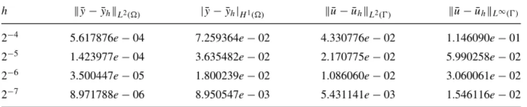
(32) 3.3. ERROR ESTIMATES. 31. ¯ ¯ ¯ ∂L ¯ ¯ (ξT , y¯h (ξT ), s¯(ξT )) − ∂L (ξT , y¯(ξT ), s¯(ξT ))¯ + ¯ ∂u ¯ ∂u ¯ ¯ ¯ ¯ ∂L ∂L ¯ (ξT , y¯(ξT ), s¯(ξT )) − ¯= (ξ , y ¯ (ξ ), s ¯ (ξ )) T h T h T ¯ ¯ ∂u ∂u ¯ ¯ ¯ ∂L ¯ ¯ (ξT , y¯h (ξT ), s¯(ξT )) − ∂L (ξT , y¯(ξT ), s¯(ξT ))¯ + |ϕ(ξ ¯ T ) − ϕ¯h (ξT )| → 0 ¯ ∂u ¯ ∂u thanks to the uniform convergence y¯h → y¯ and ϕ¯h → ϕ¯ (Lemma 3.6). ¤ In a certain way, next result is the reciprocal one to the previous theorem. The question we formulate now is wether a local minimum u of (P) can be approximated by a local minimum uh of (Ph ). The answer is positive if the local minimum u is strict. In the sequel, Bρ (u) ¯ρ (u) will denote the open ball of L∞ (Ω) with center at u and radius ρ. B will denote the corresponding closed ball. Theorem 3.8. Let us assume that (H1) and (H2) hold. Let u¯ be a strict local minimum of (P). Then there exist ε > 0 and h0 > 0 such that (Ph ) has a local minimum u¯h ∈ Bε (¯ u) for every h < h0 . Moreover the convergences (3.16) hold. Proof. Let ε > 0 be such that u¯ is the unique solution of problem ½ min J(u) (Pε ) ¯ε (¯ u∈K∩B u). Let us consider the problems ½ min Jh (uh ) (Phε ) ¯ε (¯ uh ∈ Kh ∩ B u). Let Πh : L1 (Ω) −→ Uh be the operator introduced in the proof of the ¯ε (¯ previous theorem. It is obvious that Πh u¯ ∈ Kh ∩ B u) for every h ¯ small enough. Therefore Kh ∩ Bε (¯ u) is non empty and consequently (Phε ) has at least one solution u¯h . Now we can argue as in the proof of Theorem 3.7 to conclude that k¯ uh − u¯kL∞ (Ωh ) → 0, therefore u¯h is local solution of (Ph ) in the open ball Bε (¯ u) as desired. ¤ 3.3. Error Estimates In this section we will assume that (H1) and (H2) hold and u¯ will denote a local minimum of (P) satisfying the sufficient second order condition for optimality (2.15) or equivalently (2.22). {¯ uh }h>0 will denote a sequence of local minima of problems (Ph ) such that k¯ u− u¯h kL∞ (Ωh ) → 0; remind Theorems 3.7 and 3.8. The goal of this section.

(33) 32. 3. NUMERICAL APPROXIMATION. is to estimate the error u¯ − u¯h in the norms of L2 (Ωh ) and L∞ (Ωh ) respectively. For it we are going to prove three previous lemmas. For convenience, in this section we will extend u¯h to Ω by taking u¯h (x) = u¯(x) for every x ∈ Ω. Lemma 3.9. Let δ > 0 be as in Theorem 2.12. Then there exists h0 > 0 such that (3.18). δ k¯ u − u¯h k2L2 (Ωh ) ≤ (J 0 (¯ uh ) − J 0 (¯ u))(¯ uh − u¯) ∀h < h0 . 2. Proof. Let us set ∂L d¯h (x) = (x, y¯h (x), u¯h (x)) + ϕ¯h (x) ∂u and take δ > 0 and τ > 0 as in Theorem 2.12. We know that d¯h converge uniformly to d¯ in Ω, therefore there exists hτ > 0 such that τ (3.19) kd¯ − d¯h kL∞ (Ω) < ∀h ≤ hτ . 4 For every T ∈ Th we define Z IT = d¯h (x) dx. T. From (3.10) follows. ½ u¯h |T =. α if IT > 0 β if IT < 0.. Let us take 0 < h1 ≤ hτ such that ¯ 2 ) − d(x ¯ 1 )| < τ if |x2 − x1 | < h1 . |d(x 4 This inequality along with (3.19) imply that ¯ > τ ⇒ d¯h (x) > τ ∀x ∈ T, ∀T ∈ Tˆh , ∀h < h1 , if ξ ∈ T and d(ξ) 2 hence IT > 0, therefore u¯h |T = α, in particular u¯h (ξ) = α. From (2.12) ¯ > τ and we also have u¯(ξ) = α. Then (¯ uh − u¯)(ξ) = 0 whenever d(ξ) ¯ h < h1 . We can prove the analogous result when d(ξ) < −τ . On the other hand, since α ≤ u¯h (x) ≤ β, it is obvious (¯ uh − u¯)(x) ≥ 0 if u¯(x) = α and (¯ uh − u¯)(x) ≤ 0 if u¯(x) = β. Thus we have proved that (¯ uh − u¯) ∈ Cu¯τ , remember that u¯ = u¯h in Ω \ Ωh . Then (2.22) leads to uh − u¯k2L2 (Ωh ) ∀h < h1 . (3.20) J 00 (¯ u)(¯ uh − u¯)2 ≥ δk¯ uh − u¯k2L2 (Ω) = δk¯.

(34) 3.3. ERROR ESTIMATES. 33. On the other hand, by applying the mean value theorem, we get for some 0 < θh < 1 that (J 0 (¯ uh ) − J 0 (¯ u))(¯ uh − u¯) = J 00 (¯ u + θh (¯ uh − u¯))(¯ uh − u¯)2 ≥ (J 00 (¯ u + θh (¯ uh − u¯)) − J 00 (¯ u))(¯ uh − u¯)2 + J 00 (¯ u)(¯ uh − u¯)2 ≥ (δ − kJ 00 (¯ u + θh (¯ uh − u¯)) − J 00 (¯ u)k) k¯ uh − u¯k2L2 (Ω) . Finally it is enough to choose 0 < h0 ≤ h1 such that kJ 00 (¯ u + θh (¯ uh − u¯)) − J 00 (¯ u)k ≤. δ ∀h < h0 2. to deduce (3.18). The last inequality can be obtained easily from the relationship (2.5) thanks to the uniform convergence (ϕ¯h , y¯h , u¯h ) → (ϕ, ¯ y¯, u¯) and hypothesis (H1). ¤ The next step consists in estimating the convergence of Jh0 to J 0 . Lemma 3.10. There exists a constant C > 0 independent of h such that for every u1 , u2 ∈ K and every v ∈ L2 (Ω) the following inequalities are fulfilled © ª (3.21) |(Jh0 (u2 ) − J 0 (u1 ))v| ≤ C h + ku2 − u1 kL2 (Ω) kvkL2 (Ω) .. Proof. By using the expression of the derivatives given by (2.4) and (3.5) along with the inequality (3.1) we get ¯ ¯ Z ¯ ¯ ∂L ¯ (x, yu1 , u1 ) + ϕu1 ¯ |v| dx ≤ |(Jh0 (u2 ) − J 0 (u1 ))v| ≤ ¯ ¯ Ω\Ωh ∂u ¶ µ ¶¯ Z ¯µ ¯ ∂L ¯ ∂L ¯ ¯ |v| dx ≤ (x, y (u ), u ) + ϕ (u ) − (x, y , u ) + ϕ h 2 2 h 2 u 1 u 1 1 ¯ ∂u ¯ ∂u Ωh © ª C h + kϕh (u2 ) − ϕu1 kL2 (Ω) + kyh (u2 ) − yu1 kL2 (Ω) kvkL2 (Ω) . Now (3.21) follows from the previous inequality and (3.14).. ¤. A key point in the derivation of the error estimate is to get a good approximate of u¯ by a discrete control uh ∈ Kh satisfying J 0 (¯ u)¯ u = 0 J (¯ u)uh . Let us define this control uh and prove that it fulfills the required conditions. For every T ∈ Th let us set Z ¯ dx. d(x) IT = T.

(35) 34. 3. NUMERICAL APPROXIMATION. We define uh ∈ Uh with uh|T = uhT for every T ∈ Th given by the expression Z  1  ¯ u(x) dx si IT 6= 0 d(x)¯    IT T (3.22) uhT = Z   1   u¯(x) dx si IT = 0. m(T ) T We extend this function to Ω by taking uh (x) = u¯(x) for every x ∈ Ω \ Ωh . This function uh satisfies our requirements. Lemma 3.11. There exists h0 > 0 such that for every 0 < h < h0 the following properties hold (1) uh ∈ Kh . (2) J 0 (¯ u)¯ u = J 0 (¯ u)uh . (3) There exists C > 0 independent of h such that (3.23). k¯ u − uh kL∞ (Ωh ) ≤ Ch.. Proof. Let Λu¯ > 0 be the Lipschitz constant of u¯ and let us take h0 = (β − α)/(2Λu¯ ), then for every T ∈ Th and every h < h0 β−α ∀ξ1 , ξ2 ∈ T |¯ u(ξ2 ) − u¯(ξ1 )| ≤ Λu¯ |ξ2 − ξ1 | ≤ Λu¯ h < 2 which implies that u¯ cannot take the values α and β in a same element T for any h < h0 . Therefore the sign of d¯ in T must be constant thanks ¯ = 0 for all x ∈ T . Moreover to (2.12). Hence IT = 0 if and only if d(x) ¯ if IT 6= 0, then d(x)/I T ≥ 0 for every x ∈ T . As a first consequence of this we get that α ≤ uhT ≤ β, which means that uh ∈ Kh . On the other hand ¶ Z X µZ 0 ¯ ¯ J (¯ u)uh = d(x)¯ uh (x) dx + d(x) dx uhT Ω\Ωh. Z. ¯ u(x) dx + d(x)¯. = Ω\Ωh. T ∈Th. XZ T ∈Th. T. ¯ u(x) dx = J 0 (¯ d(x)¯ u)¯ u. T. ¯ Finally let us prove (3.23). Since the sign of d(x)/I T is always non ¯ negative and d is a continuous function, we get for any of the two possible definitions of uhT the existence of a point ξ j ∈ T such that uhT = u¯(ξj ). Hence for all x ∈ T |¯ u(x) − uh (x)| = |¯ u(x) − uhT | = |¯ u(x) − u¯(ξ j )| ≤ Λu¯ |x − ξ j | ≤ Λu¯ h, which proves (3.23). Finally we get the error estimates.. ¤.

(36) 3.3. ERROR ESTIMATES. 35. Theorem 3.12. There exists a constant C > 0 independent of h such that (3.24). k¯ u − u¯h kL2 (Ω) ≤ Ch.. Proof. Taking u = u¯h in (2.9) we get ¶ Z µ ∂L 0 ϕ¯ + (x, y¯, u¯) (¯ uh − u¯) dx ≥ 0. (3.25) J (¯ u)(¯ uh − u¯) = ∂u Ω From (3.10) with uh defined by (3.22) it follows ¶ Z µ ∂L 0 ϕ¯h + Jh (¯ uh )(uh − u¯h ) = (x, y¯h , u¯h ) (uh − u¯h ) dx ≥ 0, ∂u Ω then (3.26). Jh0 (¯ uh )(¯ u − u¯h ) + Jh0 (¯ uh )(uh − u¯) ≥ 0.. Adding (3.25) and (3.26) and using Lemma 3.11-2, we deduce (J 0 (¯ u) − Jh0 (¯ uh )) (¯ u − u¯h ) ≤ Jh0 (¯ uh )(uh − u¯) = (Jh0 (¯ uh ) − J 0 (¯ u)) (uh − u¯). For h small enough, this inequality along with (3.18) imply δ k¯ u − u¯h k2L2 (Ω) ≤ (J 0 (¯ u) − J 0 (¯ uh )) (¯ u − u¯h ) ≤ 2 (Jh0 (¯ uh ) − J 0 (¯ uh )) (¯ u − u¯h ) + (J 0 (¯ uh ) − J 0 (¯ u)) (uh − u¯). Using (3.21) with u2 = u1 = u¯h and v = u¯ − u¯h in the first addend of the previous line and th expression of J 0 given by (2.4) along with (3.14) for v = u¯ and vh = u¯h , in the second addend, it comes δ k¯ u − u¯h k2L2 (Ω) ≤ C1 hk¯ u − u¯h kL2 (Ω) + 2 ¡ ¢ C2 h2 + k¯ u − u¯h kL2 (Ω) k¯ u − uh kL2 (Ω) . From (3.23) and by using Young’s inequality in the above inequality we deduce δ δ k¯ u − u¯h k2L2 (Ωh ) = k¯ u − u¯h k2L2 (Ω) ≤ C3 h2 , 4 4 which implies (3.24). ¤ Finally let us prove the error estimates in L∞ (Ω). Theorem 3.13. There exists a constant C > 0 independent of h such that (3.27). k¯ u − u¯h kL∞ (Ωh ) ≤ Ch..

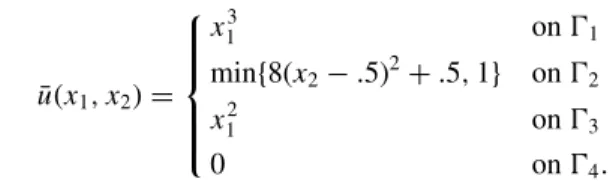
(37) 36. 3. NUMERICAL APPROXIMATION. Proof. Let ξT be defined by (3.17). In the proof of Theorem 3.3 we obtained k¯ u − u¯h kL∞ (Ωh ) ≤ k¯ s − s¯h kL∞ (Ωh ) ≤ Λs¯h+ ¯ ¯ ¯ ∂L ¯ ∂L ¯ max ¯ (ξT , y¯h (ξT ), s¯(ξT )) − (ξT , y¯(ξT ), s¯(ξT ))¯¯ + |ϕ(ξ ¯ T ) − ϕ¯h (ξT )|. T ∈Th ∂u ∂u Using the hypothesis (H1), (3.15) and (3.24) we get k¯ u − u¯h kL∞ (Ωh ) ≤ Λs¯h + C(k¯ y − y¯h kL∞ (Ω) + kϕ¯ − ϕ¯h kL∞ (Ω) ) ≤ Λs¯h + C(h + k¯ u − u¯h kL2 (Ωh ) ) ≤ Ch. ¤ Remark 3.14. Error estimates for problems with pointwise state constraints is an open problem. The reader is referred to Deckelnick and Hinze [32] for the linear quadratic case, when one side pointwise state constraints and no control constraints. The case of integral state constraints has been studied by Casas [17]. In Casas [18], the approximation of the control problem was done by using piecewise linear continuous functions. For these approximations the error estimate can be improved. The case of Neumann boundary controls has been studied by Casas, Mateos and Tröltzsch [26] and Casas and Mateos [24]. Casas and Raymond considered the case of Dirichlet controls [27]..

(38) Bibliography 1. F. Abergel and E. Casas, Some optimal control problems of multistate equations appearing in fluid mechanichs, RAIRO Modél. Math. Anal. Numér. 27 (1993), no. 2, 223–247. 2. N. Arada, E. Casas, and F. Tröltzsch, Error estimates for the numerical approximation of a semilinear elliptic control problem, Comp. Optim. Appls. 23 (2002), no. 2, 201–229. 3. E. Di Benedetto, On the local behaviour of solutions of degenerate parabolic equations with measurable coefficients, Ann. Scuola Norm. Sup. Pisa Cl. Sci. (4) 13 (1986), no. 3, 487–535. 4. J.F. Bonnans and E. Casas, Contrˆ ole de systèmes elliptiques semilinéaires comportant des contraintes sur l’état, Nonlinear Partial Differential Equations and Their Applications. Collège de France Seminar (H. Brezis and J.L. Lions, eds.), vol. 8, Longman Scientific & Technical, New York, 1988, pp. 69–86. 5. , Optimal control of semilinear multistate systems with state constraints, SIAM J. Control Optim. 27 (1989), no. 2, 446–455. 6. , Optimal control of state-constrained unstable systems of elliptic type, Control of Partial Differential Equations (Berlin-Heidelberg-New York) (A. Berm´ udez, ed.), Springer-Verlag, 1989, Lecture Notes in Control and Information Sciences 114, pp. 84–91. 7. , Un principe de Pontryagine pour le contrˆ ole des systèmes elliptiques, J. Differential Equations 90 (1991), no. 2, 288–303. 8. , An extension of Pontryagin’s principle for state-constrained optimal control of semilinear elliptic equations and variational inequalities, SIAM J. Control Optim. 33 (1995), no. 1, 274–298. 9. J.F. Bonnans and H. Zidani, Optimal control problems with partially polyhedric constraints, SIAM J. Control Optim. 37 (1999), no. 6, 1726–1741. 10. H. Brezis, An´ alisis funcional, Alianza Editorial, Madrid, 1984. 11. E. Casas, Optimality conditions and numerical approximations for some optimal design problems, Control Cybernet. 19 (1990), no. 3–4, 73–91. 12. , Optimal control in coefficients with state constraints, Appl. Math. Optim. 26 (1992), 21–37. , Pontryagin’s principle for optimal control problems governed by semi13. linear elliptic equations, International Conference on Control and Estimation of Distributed Parameter Systems: Nonlinear Phenomena (Basel) (F. Kappel and K. Kunisch, eds.), vol. 118, Int. Series Num. Analysis. Birkhäuser, 1994, pp. 97–114. , Control problems of turbulent flows, Flow Control (M.D. Gunzburger, 14. ed.), IMA Volumes in Applied Mathematics and its Applications, Springer– Verlag, 1995, pp. 127–147. 37.

(39) 38. 15.. 16.. 17.. 18. 19.. 20. 21.. 22.. 23. 24. 25.. 26.. 27.. 28.. 29. 30.. 31.. BIBLIOGRAPHY. , Pontryagin’s principle for state-constrained boundary control problems of semilinear parabolic equations, SIAM J. Control Optim. 35 (1997), no. 4, 1297–1327. , An optimal control problem governed by the evolution Navier-Stokes equations, Optimal Control of Viscous Flows (Philadelphia) (S.S. Sritharan, ed.), Frontiers in Applied Mathematics, SIAM, 1998. , Error estimates for the numerical approximation of semilinear elliptic control problems with finitely many state constraints, ESAIM:COCV 8 (2002), 345–374. , Using piecewise linear functions in the numerical approximation of semilinear elliptic control problems, Adv. Comp. Math. (To appear. 2005). E. Casas and L.A. Fern´ andez, Distributed control of systems governed by a general class of quasilinear elliptic equations, J. Differential Equations 104 (1993), no. 1, 20–47. , Dealing with integral state constraints in control problems of quasilinear elliptic equations, SIAM J. Control Optim. 33 (1995), no. 2, 568–589. E. Casas, O. Kavian, and J.-P. Puel, Optimal control of an ill-posed elliptic semilinear equation with an exponential non linearity, ESAIM: COCV 3 (1998), 361–380. E. Casas and M. Mateos, Second order optimality conditions for semilinear elliptic control problems with finitely many state constraints, SIAM J. Control Optim. 40 (2002), no. 5, 1431–1454. , Uniform convergence of the FEM. Applications to state constrained control problems, Comp. Appl. Math. 21 (2002), no. 1, 67–100. , Error estimates for the numerical approximation of Neumann control problems, Comp. Optim. Appls. (To appear). E. Casas, M. Mateos, and J.-P. Raymond, Error estimates for the numerical approximation of a distributed control problem for the steady-state navier-stokes equations, SIAM J. on Control & Optim. (To appear). E. Casas, M. Mateos, and F. Tröltzsch, Error estimates for the numerical approximation of boundary semilinear elliptic control problems, Comp. Optim. Appls. 31 (2005), 193–219. E. Casas and J.-P. Raymond, Error estimates for the numerical approximation of Dirichlet boundary control for semilinear elliptic equations, SIAM J. on Control & Optim. (To appear). E. Casas, J.P. Raymond, and H. Zidani, Optimal control problems governed by semilinear elliptic equations with integral control constraints and pointwise state constraints, International Conference on Control and Estimations of Distributed Parameter Systems (Basel) (W. Desch, F. Kappel, and K. Kunisch Eds., eds.), vol. 126, Int. Series Num. Analysis. Birkhäuser, 1998, pp. 89–102. , Pontryagin’s principle for local solutions of control problems with mixed control-state constraints, SIAM J. Control Optim. 39 (2000), no. 4, 1182–1203. E. Casas and F. Tröltzsch, Second order necessary and sufficient optimality conditions for optimization problems and applications to control theory, SIAM J. Optim. 13 (2002), no. 2, 406–431. E. Casas and J. Yong, Maximum principle for state–constrained optimal control problems governed by quasilinear elliptic equations, Differential Integral Equations 8 (1995), no. 1, 1–18..