HAL Id: tel-02094292
https://tel.archives-ouvertes.fr/tel-02094292
Submitted on 9 Apr 2019HAL is a multi-disciplinary open access archive for the deposit and dissemination of sci-entific research documents, whether they are pub-lished or not. The documents may come from teaching and research institutions in France or abroad, or from public or private research centers.
L’archive ouverte pluridisciplinaire HAL, est destinée au dépôt et à la diffusion de documents scientifiques de niveau recherche, publiés ou non, émanant des établissements d’enseignement et de recherche français ou étrangers, des laboratoires publics ou privés.
Bassel Marhaba
To cite this version:
Bassel Marhaba. Satellite image restoration by nonlinear statistical filtering techniques. Automatic Control Engineering. Université du Littoral Côte d’Opale, 2018. English. �NNT : 2018DUNK0502�. �tel-02094292�
École doctorale n° 072 : Sciences Pour l'Ingénieur Unité de recherche : LISIC
THESE
Présentée par :
Bassel MARHABA
Pour obtenir le grade de
Docteur de l’Université du Littoral Côte d'Opale
Spécialité : Automatique, Génie informatique, Traitement du Signal et des Image
Titre de la thèse
Restauration d'images Satellitaires par des
techniques de filtrage statistique non linéaire
Soutenu le 21 Novembre 2018, devant le jury composé de :
Président du jury
Mme. Christine Fernandez-Maloigne, Professeur à l’Université de Poitiers
Rapporteurs
M. Yassine Ruichek, Professeur à l’Université de Technologie de Belfort-Montbéliar M. Stéphane Derrode, Professeur à l’École Centrale de Lyon
Examinateurs
M. Abdelmalik Taleb-Ahmed, Professeur à l’IUT de Valenciennes M. Ayman Al Falou, Professeur à Yncréa Ouest/ISEN
Directeur de thèse
École doctorale n° 072: Sciences Pour l'Ingénieur SPI Research Unit: LISIC
THESE
presented by:
Bassel MARHABA
To obtain the grade of
Doctor from the Université du Littoral Côte d'Opale
Specialty: Automatic, Computer Engineering, Signal and Image Processing.Thesis Title
Satellite image restoration by nonlinear statistical
filtering techniques
Defended on November 21st, 2018, in front of the jury composed of: President of the jury
Mrs. Christine Fernandez-Maloigne, professor at the University of Poitiers
Rapporteurs
Mr. Yassine Ruichek, Professor at Belfort-Montbéliar University of Technology Mr. Stéphane Derrode, professor at the Ecole Centrale de Lyon
Examiners
Mr. Abdelmalik Taleb-Ahmed, professor at the IUT of Valenciennes Mr. Ayman Al Falou, Professor at Yncrea West / ISEN
Thesis supervisor
v
Résumé
Le traitement des images satellitaires est considéré comme l'un des domaines les plus intéressants dans les domaines de traitement d'images numériques. Les images satellitaires peuvent être dégradées pour plusieurs raisons, notamment les mouvements des satellites, les conditions météorologiques, la dispersion et d’autres facteurs. Plusieurs méthodes d'amélioration et de restauration des images satellitaires ont été étudiées et développées dans la littérature. Les travaux présentés dans cette thèse se concentrent sur la restauration des images satellitaires par des techniques de filtrage statistique non linéaire. Dans un premier temps, nous avons proposé une nouvelle méthode pour restaurer les images satellitaires en combinant les techniques de restauration aveugle et non aveugle. La raison de cette combinaison est d'exploiter les avantages de chaque technique utilisée. Dans un deuxième temps, de nouveaux algorithmes statistiques de restauration d'images basés sur les filtres non linéaires et l'estimation non paramétrique de densité multivariée ont été proposés. L'estimation non paramétrique de la densité à postériori est utilisée dans l'étape de ré-échantillonnage du filtre Bayésien bootstrap pour résoudre le problème de la perte de diversité dans le système de particules. Enfin, nous avons introduit une nouvelle méthode de combinaison hybride pour la restauration des images basée sur la transformée en ondelettes discrète (TOD) et les algorithmes proposés à l’étape deux, et nous avons prouvé que les performances de la méthode combinée sont meilleures que les performances de l’approche TOD pour la réduction du bruit dans les images satellitaires dégradées.
Mots-clés : Image satellitaire, Restauration, techniques de restauration aveugle et non aveugle,
filtre Bayésien bootstrap, estimation non paramétrique de densité multivariée, TOD.
Abstract
Satellite image processing is considered one of the more interesting areas in the fields of digital image processing. Satellite images are subject to be degraded due to several reasons, satellite movements, weather, scattering, and other factors. Several methods for satellite image enhancement and restoration have been studied and developed in the literature. The work presented in this thesis, is focused on satellite image restoration by nonlinear statistical filtering techniques. At the first step, we proposed a novel method to restore satellite images using a combination between blind and non-blind restoration techniques. The reason for this combination is to exploit the advantages of each technique used. In the second step, novel statistical image restoration algorithms based on nonlinear filters and the nonparametric multivariate density estimation have been proposed. The nonparametric multivariate density estimation of posterior density is used in the resampling step of the Bayesian bootstrap filter to resolve the problem of loss of diversity among the particles. Finally, we have introduced a new hybrid combination method for image restoration based on the discrete wavelet transform (DWT) and the proposed algorithms in step two, and, we have proved that the performance of the combined method is better than the performance of the DWT approach in the reduction of noise in degraded satellite images.
Key words: Satellite image, Restoration, blind and non-blind restoration techniques, Bayesian
vii
Dans la vie, rien n'est gratuit. Pour obtenir quelque chose, vous devez payer
pour cela. Ce travail dans vos mains - comme tout - n'était pas gratuit, le
prix était le sacrifice, l'effort et les larmes.
In this life nothing is free. In order to get something, you have to pay for it.
This work in your hands - like everything - was not for free, the price was
sacrifice, effort, and tears.
ix
Remerciements
Je voudrais exprimer ma profonde gratitude à mon directeur, M. Mourad ZRIBI. C'était une belle collaboration. Il était toujours là où il devrait être. J'ai beaucoup bénéficié de lui, non seulement dans le domaine scientifique, mais aussi dans de nombreux aspects de la vie. Avec ses connaissances et son attention, il était toujours le superviseur expert et le frère assistant. Sans son aide, je ne pourrais jamais terminer mes recherches.
Je remercie vivement mes rapporteurs de thèse, M. Yassine RUICHEK et M. Stéphane DERRODE pour le temps qu’ils ont consacré à la lecture ainsi que pour la qualité de leur expertise et de leurs critiques constructives qui ont grandement permis d’améliorer la version finale de ce travail.
Je suis très reconnaissant à Mme Christine FERNANDEZ-MALOIGNE, M. Abdelmalik TALEB-AHMED et M. Ayman Al FALOU pour prendre part à mon jury de thèse et de leurs conseils et je les remercie sincèrement.
Je voudrais également remercier tous mes amis du laboratoire pour la bonne ambiance qui a prévalu entre nous et qui a été un catalyseur supplémentaire. Merci à vous tous et je vous souhaite le meilleur dans votre vie scientifique et personnelle.
J'aimerais également remercier à tous les membres du laboratoire d'Informatique Signal et Image de la Côte d'Opale de l'Université du Littoral Côte d'Opale.
J'aimerais également remercier l'Europian Space Agency (ESA) pour avoir fourni des images satellitaires gratuitement.
Bien sûr, mes profonds remerciements à ma bonne famille. Mon père Ghazi, ma mère
Nawal, mes enfants, Zaynab, Mariam, Linah et Ghazi, ma femme Dina, ma belle- mère Bouchra, mes frères et mes beaux-frères. Vos prières, votre amour et vos soins ont
toujours été pour moi une source de force pour poursuivre ma thèse et ma vie. Dina, merci de tout cœur pour votre soutien, votre patience et votre véritable amour. Vous avez tous contribué à ce travail. Merci beaucoup.
xi
Acknowledgement
I would like to express my deep gratitude to my director, Mr. Mourad ZRIBI. It was a beautiful and adorable collaboration. He was always where he should be. I benefited greatly from him, not only in the scientific field but also in many aspects of life. With his knowledge and attention, he was always the expert supervisor and the assistant brother. Without his help, I could never finish my research.
I would like to thank my thesis reviewers, Mr. Yassine RUICHEK and Mr. Stéphane
DERRODE for the time they have devoted to reading as well as for the quality of their expertise
and their constructive criticism, which greatly improved the final version of this work.
I am very grateful to Mrs Christine FERNANDEZ-MALOIGNE, Mr Abdelmalik
TALEB-AHMED and Mr Ayman Al FALOU for taking part in my thesis jury and their
advices and I thank them sincerely.
I would also like to thank all my friends from the laboratory for the good atmosphere that has prevailed between us and which has been an additional catalyst. Thank you all and wish you the best in your scientific and personal life.
I would also like to thank all the members of the Signal and Image Computer Laboratory at the Côte d'Opale at the Côte d'Opale Coastal University.
I would also like to thank the European Space Agency (ESA) for providing free satellite images.
Of course, my deepest thanks to my good family. My father Ghazi, my mother Nawal, my children, Zaynab, Mariam, Linah and Ghazi, my wife Dina, my mother-in-law Bouchra, my
brothers and my brothers-in-law. Your prayers, your love, and your care have always been a
source of strength for me to pursue my thesis and my life. Dina, thank you wholeheartedly for your support, your patience and your true love. All of you have contributed to this work. Thank you so much.
xiii
During this thesis, 4 papers have been published in international conferences. In addition, 1 paper has been published in international journal.
Paper in International journal:
1. Bassel Marhaba, Mourad Zribi, Wassim Khoder, Image Restoration Using a Combination of Blind and Non-Blind Deconvolution Techniques, International Journal of Engineering Research & Science (IJOER), Vol. 2, No. 5, pp. 225–239, May 2016.
Papers in International conferences:
2. Bassel Marhaba, Mourad Zribi, Regularized bootstrap filter for image restoration, 11th International Conferences Computer Graphics, Visualization, Computer Vision and Image Processing and Big Data Analytics, Data Mining and Computational Intelligence, Lisbon, pp. 117-123, July 2017.
3. Bassel Marhaba, Mourad Zribi, The bootstrap Kernel-Diffeomorphism Filter for Satellite Image Restoration, IEEE 22nd International Symposium on Consumer Technologies, Russia, pp. 80 - 84, May 2018.
4. Bassel Marhaba, Mourad Zribi, Reduction of speckle noise in SAR images using hybrid combination of Bootstrap filtering and DWT, International Conference on Computer and Applications (ICCA), Beirut, pp. 377-382, July 2018.
5. Bassel Marhaba, Mourad Zribi, A Novel Combination Method for Image Restoration Based on Bootstrap Filter and DWT, Accepted in 5th International Francophone Congress of Advanced Mechanics (CIFMA), Beirut, November 2018.
xv Résumé ……….……….………..……..….v Remerciements ...……….…..…....…ix Acknowledgments ...……….…….…xi Publications...……….……….…….…xiii Table of contents ……….……...xv
List of Figures .………...……....xvii
List of Tables ……..……….………....xxi
List of Line Charts ………..……….……….xxiii
General Introduction ………...1
Chapter 1 Modeling of degraded satellite images .………...………5
Introduction ... 9
1.1 Satellite images ... 10
1.2 Reasons for image degradation ... 15
1.3 Image and degradation models ... 31
Conclusion ... 39
References ... 40
Chapter 2 Modeling of degraded satellite images ………….……… 45
Introduction ... 49
2.1 Basic model of image restoration ... 50
2.2 Non-blind restoration technique ... 52
2.3 Blind Deconvolution Methods ... 59
2.4 Proposed method to restore the Sentinel images ... 67
Conclusion ... 101
References ... 103
Chapter 3 Importance sampling Monte Carlo filters for satellite image
s
restoration………....…..107
Introduction ... 111
3.1 Analytical methods for filtering ... 112
3.2 Monte Carlo methods for nonlinear filtering ... 125
3.3 Experimental results ... 137
xvi
Introduction ... 155
4.1 Nonparametric multivariate density estimation ... 156
4.2 A proposed method to reduce the speckle noise ... 162
4.3 Experimental results ... 170
Conclusion ... 180
References ... 182
General Conclusions and Prespectives ... 187
xvii
List of Figures
Figure 1.1: The Sentinel family. ... 11
Figure 1.2: The Sentinel-1 Satellite. ... 13
Figure 1.3: The Sentinel-2 satellite. ... 15
Figure 1.4: Satellite photography. ... 18
Figure 1.5: Images and histograms corresponding to motion blurring. ... 19
Figure 1.6: Images and histograms corresponding to out-of-focus blurring. ... 21
Figure 1.7: Images and histograms corresponding to atmospheric turbulence blurring. ... 23
Figure 1.8: Images and histograms corresponding to salt and pepper noising. ... 25
Figure 1.9: Probability density function of Gaussian noise. ... 26
Figure 1.10: Images and Histograms corresponding to Gaussian noise. ... 27
Figure 1.11: Probability density function of speckle noise. ... 28
Figure 1.12: Images and histograms corresponding to speckle noise. ... 29
Figure 1.13: Images and histograms corresponding to Poisson noise. ... 31
Figure 1.14: The state vector x(m, n)……….33
Figure 2.1: Image degradation model. ... 50
Figure 2.2: Image restoration model. ... 51
Figure 2.3: Classification of restoration techniques. ... 52
Figure 2.4: General block diagram for image restoration. ... 52
Figure 2.5: Deblurring using Lucy-Richardson method. ... 54
Figure 2.6: Deblurring by Inverse Filter. ... 55
Figure 2.7: Deblurring by Wiener filter. ... 57
Figure 2.8: Deblurring by Regularized Filter. ... 58
Figure 2.9: Deblurring by Constrained Least-Squares filter. ... 59
Figure 2.10: Deblurring by different mean filters. ... 61
Figure 2.11: Deblurring by Median filter. ... 62
Figure 2.12: Deblurring by DWT filter. ... 64
Figure 2.13: Deblurring by bilateral filter. ... 65
Figure 2.14: Deblurring by adaptive local filter. ... 66
Figure 2.15: Proposed method for image restoration diagram. ... 68
Figure 2.16: The resultant deblurred images by the non-blind deconvolution methods and the corresponding histogram for each deblurred image, for the motion blur case. ... 71
xviii
Figure 2.17: The resultant deblurred images by the blind deconvolution methods, and the corresponding histogram for each deblurred image, for the motion blur case. ... 73 Figure 2.18: The resultant deblurred images by the non-blind deconvolution methods, and the
corresponding histogram for each deblurred image, for the out of focus blur case. ... 76 Figure 2.19: The resultant deblurred images by the blind deconvolution methods, and the
corresponding histogram for each deblurred image, for the out of focus blur case. ... 78 Figure 2.20: The resultant deblurred images by the non-blind deconvolution methods and the
corresponding histogram for each deblurred image, for the atmospheric turbulence blur case. ... 80 Figure 2.21: The resultant deblurred images by the blind deconvolution methods, and the
corresponding histogram for each deblurred image, for the atmospheric turbulence blur case. ... 82 Figure 2.22: The resultant denoised images by the non-blind deconvolution methods, for the
salt & pepper noise. ... 84 Figure 2.23: The resultant denoised image by the blind deconvolution methods for the salt &
pepper noise. ... 85 Figure 2.24: The resultant denoised images by the non-blind deconvolution methods, for the
Gaussian noise. ... 87 Figure 2.25: The resultant denoised image by the blind deconvolution methods, for the Gaussian
noise. ... 87 Figure 2.26: The resultant denoised images by the non-blind deconvolution methods, for the
Speckle noise. ... 89 Figure 2.27: The resultant denoised images by the blind deconvolution methods, for the Speckle
noise. ... 89 Figure 2.28: The resultant denoised images by the non-blind deconvolution methods, for the
Poisson noise. ... 91 Figure 2.29: The resultant denoised image by the blind deconvolution methods, for the Poisson
noise. ... 91 Figure 2.30: The resultant restored images by the non-blind deconvolution methods, for the case
of atmospheric turbulence blur and Speckle noise. ... 93 Figure 2.31: The resultant restored image by the blind deconvolution methods, for the case of
xix
Figure 2.34: The resultant restored image, for the atmospheric turbulence blur. ... 97
Figure 2.35: The resultant restored image, for the salt & pepper noise. ... 98
Figure 2.36: The resultant restored image for the Gaussian noise. ... 99
Figure 2.37: The resultant restored image for the speckle noise. ... 99
Figure 2.38: The resultant restored image for the Poisson noise. ... 100
Figure 2.39: The resultant restored image for the Speckle noise with atmospheric turbulence blur. ... 101
Figure 3.1: Restoration of the French synergy image degraded by impulse noise. ... 139
Figure 3.2: Restoration of the Seville Spain image degraded by the impulse noise. ... 140
Figure 3.3: Restoration of the French synergy image degraded by the Gaussian noise. ... 141
Figure 3.4: Restoration of the Seville Spain image degraded by the Gaussian noise. ... 142
Figure 3.5: Restoration of the Seville Spain image degraded by the Gaussian noise. ... 143
Figure 3.6: Restoration of the Seville Spain image degraded by the Gaussian noise. ... 144
Figure 4.1: Kernel density estimate with diagonal bandwidth for synthetic normal mixture data. ... 159
Figure 4.2: Estimation of pdf . ... 161
Figure 4.3: The Proposed algorithm. ... 163
Figure 4.4: ERS SAR image. ... 164
Figure 4.5: Noised SAR image... 165
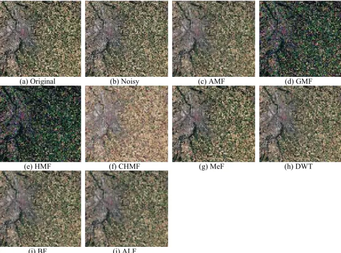
Figure 4.6: Denoising of ‘Sydney, Australia’ image corrupted by speckle noise of variance of 0.08. ... 174
Figure 4.7: Denoising of ‘city of Paris’ image corrupted by speckle noise of variance of 0.08. . ... 179
) (
, x
xxi
Table 2.1: The resultant metrics of the deblurred by non-blind deconvolution methods for the motion blur case. ... 74 Table 2.2: The resultant metrics of the deblurred by blind deconvolution methods for the motion
blur case. ... 74 Table 2.3: The resultant metrics of the deblurred by non-blind deconvolution methods, for the
out of focus blur case. ... 78 Table 2.4: The resultant metrics of the deblurred by blind deconvolution methods, for the out
of focus blur case. ... 78 Table 2.5: The resultant metrics of the deblurred by non-blind deconvolution methods, for the
atmospheric turbulence blur case. ... 82 Table 2.6: The resultant metrics of the deblurred by blind deconvolution methods, for the
atmospheric turbulence blur case. ... 83 Table 2.7: The resultant metrics of the denoised by non-blind deconvolution methods for the
salt & pepper noise. ... 85 Table 2.8: The resultant metrics of the denoised by the blind deconvolution methods for the salt
& pepper noise. ... 85 Table 2.9: The resultant metrics of the denoised by non-blind deconvolution methods, for the
Gaussian noise. ... 88 Table 2.10: The resultant metrics of the denoised by the blind deconvolution methods, for the
Gaussian noise. ... 88 Table 2.11: The resultant metrics of the denoised by non-blind deconvolution methods, for the
Speckle noise. ... 90 Table 2.12: The resultant metrics of the denoised by the blind deconvolution methods, for the
Speckle noise. ... 90 Table 2.13: The resultant metrics of the denoised by non-blind deconvolution methods, for the
Poisson noise. ... 92 Table 2.14: The resultant metrics of the denoised by the blind deconvolution methods, for the
Poisson noise. ... 92 Table 2.15: The resultant metrics of the restoration with non-blind deconvolution methods, for
xxii
Table 2.17: The resultant PSNR of the different methods for the case of motion blur. ... 95 Table 2.18: The resultant PSNR of the different methods for the out of focus blur. ... 96 Table 2.19: The resultant PSNR of the different methods, for the atmospheric turbulence blur. ... 97 Table 2.20: The resultant PSNR of the different methods, for the salt & pepper noise. ... 98 Table 2.21: The resultant PSNR of the different methods for the Gaussian noise. ... 99 Table 2.22: The resultant PSNR of the different methods for the speckle noise. ... 99 Table 2.23: The resultant PSNR of the different methods for the Poisson noise. ... 100 Table 2.24: The resultant PSNR of the different methods for the Speckle noise with atmospheric
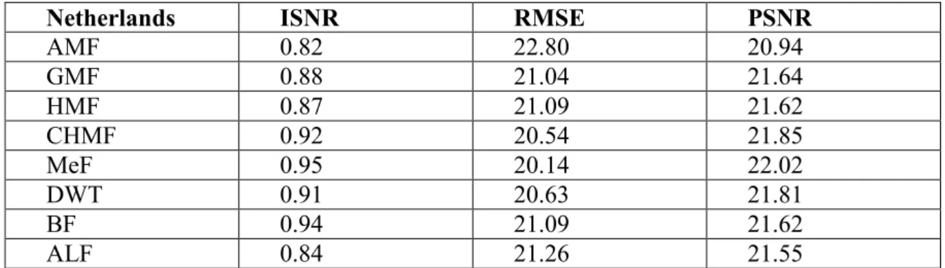
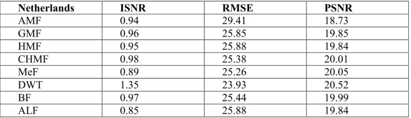
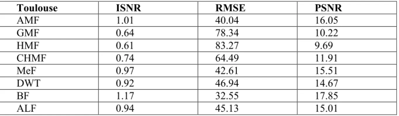
turbulence blur. ... 101 Table 3.1: The values of the images coefficients. ... 138 Table 3.2: The metric results obtained from the denoised French synergy image. ... 145 Table 3.3: The metric results obtained from the denoised Seville Spain image. ... 145 Table 4.1: Model coefficients for the used SAR images. ... 171 Table 4.2: Comparison of the ISNR resultant values of the proposed, NBBF, BBF and the other
basic filters for denoising the SAR image of Sydney corrupted by Speckle noise. ... 175 Table 4.3: Comparison of the RMSE resultant values of the proposed, NBBF, BBF and the other
basic filters for denoising the SAR image of Sydney corrupted by Speckle noise ... 175 Table 4.4: Comparison of the PSNR resultant values of the proposed, NBBF, BBF and the other
basic filters for denoising the SAR image of Sydney corrupted by Speckle noise. ... 175 Table 4.5: Comparison of ISNR resultant values of the proposed, NBBF, BBF and other basic
filters for denoising the SAR image of Paris corrupted by Speckle noise. ... 179 Table 4.6: Comparison of RMSE resultant values of the proposed, NBBF, BBF and other basic
filters for denoising the SAR image of Paris corrupted by Speckle noise. ... 179 Table 4.7: Comparison of PSNR resultant values of the proposed, NBBF, BBF and other basic
xxiii
List of Line Charts
Line Chart 4.1: The PSNR results for denoising the SAR image of Sydney by the several filters. ... 176 Line Chart 4.2: The PSNR results for denoising the image of the city of Paris SAR image by
1
Satellite imagery, space-borne photography, or remote sensing, are different names for the images of Earth or other planets collected by imaging satellites operated by governments and businesses around the world in order to obtain information about the regions been photographed. Then these companies sell images by licensing them to governments and other private organizations such as Apple Maps and Google Maps.
There are many different satellites scanning the Earth, each with its own unique purpose. Satellites use different kinds of sensors to collect electromagnetic radiation reflected from the Earth. Passive sensors collect radiation which the Sun emits and the Earth reflects, and do not require energy. Active sensors emit radiation themselves, and analyze it after it is reflected back from the Earth. Active sensors require a significant amount of energy to emit radiation, but they are useful because they can be used during any season and time of day (passive sensors cannot be used on a part of Earth that is in shadow) and because they can emit types of radiation that the Sun does not provide.
Satellite images are useful because different surfaces and objects can be identified by the way they react to radiation. For instance, smooth surfaces, such as roads, reflect almost all of the energy, which comes at them at a single direction. This is called specular reflection. Meanwhile, rough surfaces, such as trees, reflect energy in all directions. This is called diffuse reflection. Sensing different types of reflection is useful in measuring the density and amount of forests, and forest change. Also, objects react differently to different wavelengths of radiation. For instance, there is a frequency of infrared light, which can be used to determine plant health. Healthy leaves reflect this frequency well while unhealthy ones do not.
Satellite images are subject to distortion due to the presence of two disturbing factors that negatively affect the purity and clarity of the satellite images degraded by noise during image acquisition and transmission process. These two factors are blur and noise. There are many types of blur that affect satellite images, such as motion blur, out of focus blur and atmospheric turbulence blur. On the other hand, there are also several types of noise that affect the satellite images such as impulse noise, additive noise and multiplicative noise. The presence of blur and/or noise in the satellite images is a very disturbing issue since it has reduced the purity of the image and distorts the useful information in the image. These distorted images must be restored and the useful information must be recovered.
Reducing and eliminating noise and/or blur from the satellite images is a big challenge for the researchers in the domain digital image processing. The process of reducing the noise and/or blur from the satellite images and recovering the useful information in it is called; denoising in the presence of noise only, deblurring in the presence of blur only or restoration in the presence of both noise and blur which also can be called denoising, and deblurring. Anyhow, deblurring and denoising could be named restoration.
For several decades and until now, reducing noise and/or blur from the satellite images is a big hurdle for the researchers in digital image processing. Many methods were proposed and developed in the literature for restoring satellite images.
2
During our work in this thesis several contributions have been made. At the first step, we examined several blind and non-blind restoration techniques already exist in the literature. Blind image restoration techniques have no/or few knowledge about the point spread function that has degraded the original image. On the other hand, non-blind restoration techniques have a prior information about the point spread function, which has degraded the original image. During this step, we studied, tested and compared the behavior of these techniques through implementing it on restoration degraded satellite images. Here, the contribution is the fusion combination between the blind and non-blind restoration techniques based on the wavelet transform method. In the second step, we studied the Monte Carlo filters and the nonparametric multivariate density estimation for satellite image restoration. Here our first contribution is to adopt the recursive Bayesian Bootstrap filtering for image restoration. Bootstrap filter is a filtering method based on Bayesian state estimation and Monte Carlo method, which has the great advantage of being able to handle any functional non-linearity and system and/or measurement noise of any distribution. Due to the problem of degeneracy found in the (sequential importance sampling) particle filter, where after a few sampling steps all the particles except one will have a negligible weight, the bootstrap filter with a resampling step was introduced to solve the degeneracy problem. Although the resampling step in the Bayesian bootstrap filter has solved the degeneracy problem, but it has caused loss of diversity among the particles. This problem arises due to the fact that the particles are drawn from a discrete distribution. To solve this problem, we need to draw the particles from a continuous distribution. To achieve this solution, we propose to use nonparametric multivariate density estimation in the bootstrap resampling step. The second contribution is to use the nonparametric multivariate density estimation in the resampling step of the Bayesian bootstrap filter. Finally, to ameliorate the satellite image restoration using the new nonparametric filters, we have proposed a novel approach which combine the proposed filters and discrete wavelet transform (DWT). The DWT, is a robust approach and it is easy to be implemented in the image restoration field.
The thesis is instructed as follows
In chapter 1, we introduce satellite imagery and then we define the Sentinel family concept. After that, we describe the Sentinel 1 and 2 missions with some details about the satellites. Next, we describe the reason for the image degradation, and finally, we show the image model and the degradation model.
In chapter 2, we present a basic image restoration technique. We consider the restoration process as a two-dimensional convolution of true image and the point spread function. Subsequently, a strategy to reconstruct the true image given the blurred image and the point spread function is presented. Moreover, we give an overview of blind and non-blind restoration techniques, two topics that are regarded in more details in this chapter. To ameliorate the results obtained by the two techniques, we propose a new method of restoration which consists of fusion combination of the two techniques.
In chapter 3, we describe the Monte Carlo filters. First we review the analytical method for filtering, for example Kalman filter. In the second step, a comparative study of the different filters has been realized for the satellite image restoration. Finally, in this chapter, we are interested in Monte Carlo methods for nonlinear filtering and in particular the Bayesian bootstrap filter. Here, we have adopted the filter to the problem of satellite image restoration.
3
In chapter 4, we have treated the problem of the speckle noise of synthetic aperture radar images using Bayesian bootstrap filtering. First, we review the nonparametric multivariate density estimation. Secondly, we have noticed that resampling step in the Bayesian bootstrap filter which reduces the degeneracy problem introduced loss of diversity among the particles. This arises due to the fact that in the resampling step, samples are drawn from a discrete distribution. To resolve this problem, we have proposed to draw samples from an approximation method using nonparametric multivariate density estimation which allowed us to have new filters called nonparametric Bayesian bootstrap filtering. Finally, we proposed another hybrid combination method based on the nonparametric Bayesian bootstrap filter and the discrete wavelet transform (DWT) to reduce the speckle noise of synthetic aperture radar images.
Chapter 1
Modeling of degraded
satellite images
7
Table of Contents
Introduction ... 9 1.1 Satellite images ... 10 1.1.1 Sentinel family ... 10 1.1.2 Sentinel-1 ... 12 1.1.3 Sentinel-2 ... 14 1.2 Reasons for image degradation ... 15 1.2.1 Reasons for blurring ... 16 1.2.1.1 Motion blur ... 17 1.2.1.2 Out-of-focus blur ... 19 1.2.1.3 Atmospheric turbulence blur ... 21 1.2.2 Reasons for noise ... 23 1.2.2.1 Impulse noise ... 24 1.2.2.2 Additive noise ... 25 1.2.2.3 Multiplicative noise ... 27 1.2.2.4 Poisson noise ... 29 1.3 Image and degradation models ... 31 1.3.1 Image model... 32 1.3.2 Degradation models ... 33 1.3.2.1 Linear space-invariant blur models ... 34 1.3.2.2 Space-variant blur models ... 34 1.3.3 Estimation of image model coefficients ... 35 1.3.3.1 Least squares method ... 35 1.3.3.2 Yule-Walker equations ... 36 1.3.4 Measures of image restoration quality ... 37 1.3.4.1 Improvement Signal-to-noise ratio (ISNR) improvement ... 37 1.3.4.2 Mean Square Error (MSE) ... 38 1.3.4.3 Root Mean Square Error (RMSE) ... 38 1.3.4.4 Peak signal-to-noise ratio (PSNR) ... 38 Conclusion ... 39 References ... 409
Introduction
Satellite image processing is one of the leading fields in computer research. Scientists and researchers benefit from satellite images variety of fields such as meteorology, oceanography, fisheries, agriculture, biodiversity conservation, forestry, landscapes, astronomy, geology and more [Lia05][Was14][Zhe13][Yi11]. Images acquired from satellites degraded due to many effects, such as climate, weather and some other factors [Rav13]. In satellite image processing, images received from satellites contain large amounts of data for further processing or analysis. Satellite images are usually captured under a variety of situations. Each captured satellite image is, in a sense, a degraded version of the scene [Hua04]. Sources of degradation can be blur, noise aliasing and atmospheric turbulence, which have usually defective effects in its nature. However, the acquired image always represents a degraded version of the original scene due to defects in imaging and acquisition process. Removing these defects is important for most subsequent image processing tasks. There are different types of damage to take into consideration, such as noise, geometric degradation (pincushion deformation), imperfections in lighting and color (under/over exposure, saturation), and blurring. Due to defective image formation, blurring is a form of ideal image bandwidth reduction. The relative motion between the camera and the original scene, or an out of focus optical system may cause this blur. When producing aerial photographs for remote sensing, several factors will affect the images, like atmospheric turbulence, aberrations in the optical system, and relative motion between the camera and the ground, one/all of those factors will introduce blur in the images. An additional defect besides blur is noise, which affects any captured image. Noise can occur by the media which is producing the image (random absorption or dispersion effects), by recording media (sensor noise), by errors in measurement caused by the limited accuracy of the acquiring system and digital storage quantization of the data. Sudden changes in atmospheric temperature, external disturbances, and lack of acquisition of earth sensors, are another causes to add different types of noise to the acquired images [Kum14]. There are several types of earth satellites such as, NOAA, Metop and SAR, which are sending images to the satellite receivers. These images contain a fixed resolution depending on the application. The density, size, and length of the pixels are useful for analyzing information [Par99].
We start the first chapter with a state-of-the-art of satellite images, and in particular sentinel 1 and sentinel 2 images, in Section 1.1. In Section 1.2, we present a brief review of
10
reasons for image degradation. In Section 1.3, we describe the image and degradation models with non-symmetric half-plane (NSHP) regions of support.
1.1 Satellite images
Satellite imagery is indeed one of the eminent, robust and essential tools used by meteorologists. Actually, we can consider it as an eye in the sky. These images help forecasters to know the fluctuations in the climate and the changes expected to be achieved in the atmosphere as they provide a clear, precise and correct description of the events and how it is unfolding. Without satellites, predicting the weather and conducting research will be a hard challenge. Data collected at stations across the country are limited in terms of atmospheric performance. Although it is still possible to get a reasonable analysis of the data obtained, there will be a great opportunity to lose valuable pieces of information because hundreds of kilometers separate the earth stations. Satellite images help to show things that cannot be measured or seen. In addition, the satellite image is considered the truth. The data provided by the satellite images can be interpreted "firsthand". Satellite images may well reflect what is happening around the world, especially in the vast ocean of data. The data cannot be collected in some parts of the world, but without these data, the prediction will be as difficult as without satellites. There are two types of satellites in orbit around the Earth, polar and terrestrial. The geostationary satellite operating environment satellite (GOES) is still located at a fixed position on the Earth's surface at about 22,500 kilometers above the equator. Because satellites spin with the earth, they always see the same part of the earth. In contrast, polar-orbiting satellites have their orbits at lower altitudes (800-900 km). Their path is 2400 km wide centered on the path of the track. Polar-orbiting satellites are observing a new path in each orbit. Polar satellites are not useful for meteorologists because they do not observe the same area. Geostationary satellites allow meteorologists to observe the process of developing meteorology by observing the same area. As part of its plan to contribute to the Space Segment of Global Environmental and Security Monitoring (GMES), European Space Agency (ESA) is undertaking a high-resolution Optical Earth Observation mission. In the rest of this section, we will present a summary of sentinel images.
1.1.1 Sentinel family
ESA has developed a new family of missions called Sentinels specifically for the operational needs of the Copernicus program. Each Sentinel mission is based on a
11
constellation of two satellites to fulfil revisit and coverage requirements, providing robust datasets for Copernicus Services. These missions carry a range of technologies, such as radar and multi-spectral imaging instruments for land, ocean and atmospheric monitoring:
Figure 1.1: The Sentinel family.
Sentinel-1 is a polar-orbiting, all-weather, day-and-night radar imaging mission for land and ocean services. Sentinel-1A was launched on 3 April 2014 and Sentinel-1B on 25 April 2016. Both were taken into orbit on a Soyuz rocket from Europe's Spaceport in French Guiana.
Sentinel-2 is a polar-orbiting, multispectral high-resolution imaging mission for land monitoring to provide, for example, imagery of vegetation, soil and water cover, inland waterways and coastal areas. Sentinel-2 can also deliver information for emergency services. Sentinel-2A was launched on 23 June 2015 and Sentinel-2B followed on 7 March 2017.
12
Sentinel-3 is a multi-instrument mission to measure sea-surface topography, sea- and land-surface temperature, ocean color and land color with high-end accuracy and reliability. The mission will Support Ocean forecasting systems, as well as environmental and climate monitoring. Sentinel-3A was launched on 16 February 2016.
Sentinel-4 is a payload devoted to atmospheric monitoring that will be embarked upon a Meteosat Third Generation-Sounder (MTG-S) satellite in geostationary orbit.
Sentinel-5 Precursor – also known as Sentinel-5P – is the forerunner of Sentinel-5 to provide timely data on a multitude of trace gases and aerosols affecting air quality and climate. It has been developed to reduce data gaps between the Envisat satellite – in particular the Sciamachy instrument – and the launch of Sentinel-5. Sentinel-5P was taken into orbit on a Rocket launcher from the Plesetsk Cosmodrome in northern Russia on 13 October 2017.
Sentinel-5 is a payload that will monitor the atmosphere from polar orbit aboard a MetOp Second Generation satellite.
Sentinel-6 carries a radar altimeter to measure global sea-surface height, primarily for operational oceanography and for climate studies.
In our work, we were particularly interested in the first two as data for the restoration problem. We will first start with the description of sentinel-1 and then sentinel-2.
1.1.2 Sentinel-1
The first in the series, Sentinel-1, carries an advanced radar instrument to provide an all-weather, day-and-night supply of imagery of Earth’s surface. As a constellation of two satellites orbiting 180° apart, the mission images the entire Earth every six days. As well as transmitting data to a number of ground stations around the world for rapid dissemination, Sentinel-1 also carries a laser to transmit data to the geostationary European Data Relay System for continual data delivery.
Sentinel-1A was launched on 3 April 2014 and Sentinel-1B on 25 April 2016. Both were taken into orbit on a Soyuz rocket from Europe's Spaceport in French Guiana. The C-band Synthetic Aperture Radar (SAR) is built on ESA’s and Canada’s heritage SAR systems on ERS-1, ERS-2, Envisat and Radarsat.
13
Figure 1.2: The Sentinel-1 Satellite.
Sentinel-1 is observatory polar-orbiting European radar providing continuity of SAR data for operational applications. These applications include: monitoring sea ice zones and the arctic environment surveillance of marine environment monitoring land surface motion risks mapping of land surfaces; forest, water and soil, agriculture mapping in support of humanitarian aid in crisis situations. The design of Sentinel-1 with its focus on reliability, operational stability, global coverage and quick data delivery is expected to enable the development of new applications and meet the evolving needs of Copernicus. Sentinel-1 is the result of close collaboration between the ESA, the European Commission, industry, service providers and data users. Designed and built by a consortium of around 60 companies led by Thales Alenia Space and Airbus Defence and Space, it is an outstanding example of Europe’s technological excellence. Sentinel-1 is an imaging radar mission providing continuous all weather, day-and-night imagery at C-band. The Sentinel-1 constellation provides high reliability, improved revisit time, geographical coverage and rapid data dissemination to support operational applications in the priority areas of marine monitoring, land monitoring and emergency services. Sentinel-1 potentially images all global landmasses, coastal zones and shipping routes in European waters in high resolution and covers the global oceans at regular intervals. Having a primary operational mode over land and another over Open Ocean allows for a pre-programmed conflict-free operation. The main operational mode features a wide swath (250 km) with high geometric (typically 20 m Level-1 product resolution) and
14
radiometric resolutions, suitable for most applications. The Sentinel-1 Synthetic Aperture Radar (SAR) instrument may acquire data in four exclusive modes:
Stripmap (SM) - A standard SAR stripmap-imaging mode where the ground swath is illuminated with a continuous sequence of pulses, while the antenna beam is pointing to a fixed azimuth and elevation angle.
Interferometric Wide swath (IW) - Data is acquired in three swaths using the Terrain Observation with Progressive Scanning SAR (TOPSAR) imaging technique. In IW mode, bursts are synchronized from pass to pass to ensure the alignment of interferometric pairs. IW is Sentinel-1's primary operational mode over land.
Extra Wide swath (EW) - Data is acquired in five swaths using the TOPSAR imaging technique. EW mode provides very large swath coverage at the expense of spatial resolution.
Wave (WV) - Data is acquired in small stripmap scenes called "vignettes", situated at regular intervals of 100 km along track. The vignettes are acquired by alternating, acquiring one vignette at a near range incidence angle while the next vignette is acquired at a far range incidence angle. WV is Sentinel-1's operational mode over Open Ocean.
More details about sentinel-1 are given in appendix 1.A.
1.1.3 Sentinel-2
Sentinel-2 is a satellite system consisting of two polar-orbiting satellites, will help improve continuity and SPOT and Landsat multispectral range of tasks and ensure the high quality data and applications for a land monitoring operation, Services emergency and security intervention. The Sentinel line of satellites is planned to delivering land remote sensing data that are central to the European Commission’s Copernicus program; in late 2015, the Sentinel line became operational. The Sentinel-2 mission emerged as a result of close cooperation between the ESA, the European Commission, data users, service providers, and industry. The mission has been designed and built by a consortium of around 60 companies led by Airbus Defense and Space, and supported by the CNES French space agency to optimize image quality and by the DLR German Aerospace Centre to improve data recovery using optical communications.
The Sentinel-2 mission consists of two satellites developed to support vegetation, land cover, and environmental monitoring. The Sentinel-2A satellite was launched by ESA on June
15
23 2015, and operated in a sun-synchronous orbit with a 10-day repeat cycle. The current Sentinel-2A acquisition priorities are focused primarily on Europe. A second identical satellite (Sentinel-2B) was launched on March 7, 2017 and is expected to be operational for data acquisitions in 3-4 month. Together they will cover all Earth’s land surfaces, large islands, and inland and coastal waters every five days.
Figure 1.3: The Sentinel-2 satellite.
More details about sentinel 2 are given in appendix 1.B.
1.2 Reasons for image degradation
There are several modalities used to capture images, and for each modality, there are many ways to construct images. Therefore, there are many reasons and sources for image degradation. Images acquired through any modern sensors consist of variety of noises (such as thermal noise, amplifier noise, photon noise, quantization noise and cross talk), resulting from stochastic variations and deterministic distortions or shading. In addition to inherent reasons, blurring occurs in many image formation systems due to limited performance of both optical and electronic systems. The shutter speed, for example, is the main factor deciding the amount of motion blur. As blurring can significantly degrade the visual quality of images.
In digital image processing, in general, discrete model for a linear degradation caused by blurring and additive noise can be given by the following superposition summation,
16 g(x,y) h(x k,y l)f(x,y) n(x,y) M k N l
(1.1) where f(x, y) represents an original image with size ofM N pixels, g(x, y) is the degraded image which is acquired by the imaging system, n(x, y) represents an additive noise introduced by the system, and h(x-k, y-l) is the two-dimensional point spread function (PSF) of the imaging system, which, in general, can be spatially varying. More detail of PSF is given in Appendix 2.A.In the following of this section, we will study the reasons for image degradation on French synergy image [URL16]. A sentinel-2 image Figure 1.5 (a) shows La Rochelle - the capital of the Charente-Maritime department in western France - and surroundings. At the center, we can see clearly the 2.9 km long bridge connecting the city with the Île de Ré. The white lines represent the sandy beaches of the coastal area. Between the water line and the beach, silt layers and darker sand are shown, which are presented in this image captured during low tide. The La Rochelle- Île de Ré airport is visible at the north of the city. Also at top-right, it is the visible part of the Natural Reserve of the Bay of Aiguillon. It hosts hundreds of thousands of migratory water birds every year. It is an area of synergy between sea and land, freshwater and saltwater, and between humankind and nature. Since 23 June 2015, the Sentinel-2 has been in orbit as a polar-orbiting, high-resolution land monitoring satellite, supplying imagery of soil and water cover, vegetation, coastal areas and inland waterways. The size of this image is 2953 4016 3.
1.2.1 Reasons for blurring
Blurring in an image occurs because of a localized averaging of pixels, and results in the smoothing of image content. It can be caused by a number of phenomena including, relative motion between the camera and the imaged scene, defocusing or atmospheric turbulence. Blurring is usually modeled as a convolution of the image with the point spread function (PSF). We will form the blurring process model in the following way:
g(x, y) = (h*f)(x, y) + n(x, y) (1.2) Let us consider each component in a more detailed way. As for functions f(x, y) and g(x, y), everything is quite clear with them. However, as for the blurring function h(x, y) we need to say a couple of words. In the process of blurring each pixel of a source image turns into a spot
17
in case of defocusing and into a line segment (or some path) in case of a usual blurring due to movement. Alternatively, we can say otherwise, that each pixel of a blurred image is "assembled" from pixels of some nearby area of a source image. All those overlap each other, which fact results in a blurred image. The principle, according to which one pixel becomes spread, is called the blurring function.
1.2.1.1 Motion blur
Image blur can result from the subject moving while the shutter is open. Such movement results in the subject only being blurred. Most satellite imaging systems do not remain fixed over a target because they are in orbit around Earth or the Moon. Regarding the ordinary digital photos, the movement of our subject will cause blur in the image which we don't want to happen. For satellite photography, it is unavoidable that the satellite in its orbit or the Target are in motion (Figure 1.4). Once we have determined the resolution that our satellite camera needs to study a Target, we also have to keep track of image and Target motion, which can also blur the image. To avoid blurring, we do not want the scene being photographed to move by more than one pixel during the exposure time. Motion blurring can significantly degrade the visual quality of images. Motion blurring is usually modeled as a spatially invariant convolution process. The general form of motion blur function h is given as follows [Reg97]: otherwise 0 ) tan( and 2 if 1 ) , ( 2 2 y x L y x L y x h (1.3)
18
Figure 1.4: Satellite photography.
We present in Figure 1.5 a satellite image corrupted by linear motion blur with L=20 pixels and =45°.
19
Figure 1.5: Images and histograms corresponding to motion blurring.
1.2.1.2 Out-of-focus blur
To reduce noise in short exposures, the aperture size can be increased to allow more light into the camera. Increasing the aperture size reduces the depth of field portion of image that is in-focus, however, it increases the portion of the image that will be out-of-focus. For a circular aperture, a point source in a scene will be projected onto the sensor as a circular disc.
(a) Original color image (b) Blurred color image
(c) Original gray-level image (d) Blurred gray-level image
20
This disc is known as the circle of confusion. The diameter of the circle depends on the focal length, aperture number and the distance between the lens and the object being imaged [Bov05]. If an object is out-of-focus, the lens will behave like a low pass filter, removing high frequency image content. If the PSF is large relative to the wavelengths being imaged, it can be modeled using the following spatially-invariant blur,
otherwise 0 if 1 ) , ( 2 2 2 x y r r y x h (1.4)
where r is the radius of the out-of-focus blur.
21
(a) Original color image (b) Blurred color image
(c) Original gray-level image (d) Blurred gray-level image
(e) Histogram of image (c) (f) Histogram of image (d)
Figure 1.6: Images and histograms corresponding to out-of-focus blurring.
1.2.1.3 Atmospheric turbulence blur
Satellite images through the atmosphere are blurred, distorted, and have reduced contrast relative to their source. There are atmospheric phenomena that give rise to attenuation of the irradiance of the propagating image, thus reducing the contrast of the final image. Absorption
22
and large angle scattering by aerosols attenuate images propagating through the atmosphere [Li07]. They are blurred by small angle scattering caused by aerosols, and by optical turbulence. Image blur through the atmosphere [Li08] involves both turbulence and small angle forward scatter of light by aerosols, which is also called the adjacency effect, since it causes photons to be imaged in pixels adjacent to those in which they ought to have been imaged.
Common in remote sensing and aerial imaging, the blur due to long-term exposure though the atmosphere can be modeled by a Gaussian PSF,
) 2 exp( ) , ( 2 2 2 y x K y x h (1.5)
where K is a normalizing constant ensuring that, the blur is of unit volume, and
2is thevariance that determines the severity of the blur.
23
(a) Original color image (b) Blurred color image
(c) Original gray-level image (d) Blurred gray-level image
(e) Histogram of image (c) (f) Histogram of image (d)
Figure 1.7: Images and histograms corresponding to atmospheric turbulence blurring. 1.2.2 Reasons for noise
Digital images are prone to a variety of types of noise. Noise is the result of errors in the image acquisition process that result in pixel values that do not reflect the true intensities of the real scene [Gag96][Fed17]. There are several ways that noise can be introduced into an image, depending on how the image is created. For example, if the image is scanned from a photograph made on film, the film grain is a source of noise. Noise can also be the result of
24
damage to the film, or be introduced by the scanner itself. If the image is acquired directly in a digital format, the mechanism for gathering the data (such as a CCD detector) can introduce noise. Electronic transmission of image data can introduce noise. Noise is deemed to be each or any measurement that is not part of the phenomena of importance. In imagery, we can categorize the noise into two categories as image data independent noise and image data dependent noise. Noise could be added systematically introduced into images. As types of noise, there are three types which are mostly represented to be added to the image; impulse, additive and multiplicative noise [Sub11].
1.2.2.1 Impulse noise
Impulse noise [Har10][Ric17] corruption is very common in digital images. Impulse noise is always independent and uncorrelated to the image pixels and is randomly distributed over the image. Hence unlike Gaussian noise, for an impulse noise corrupted image all the image pixels are not noisy, a number of image pixels will be noisy and the rest of pixels will be noise free. There are different types of impulse noise namely salt and pepper type of noise and random valued impulse noise. In salt and pepper type of noise the noisy pixels take either salt value (gray level-225) or pepper value (grey level-0) and it appears as black and white spots on the images. If p is the total noise density then, salt noise and pepper noise will have a noise density of p/2. This can be mathematically represented by:
p j i f p j i g 1 y probabilit with ) , ( y probabilit with 255 or 0 ) , ( (1.6)
where g(i, j) represents the noisy image pixel, p is the total noise density of impulse noise and f(i, j) is the uncorrupted image pixel.
At times the salt noise and pepper noise may have different noise densities p1 and p2 and the total noise density will be p=p1+ p2. In case of random valued impulse noise, noise can take any gray level value from 0 to 225. In this case, also, noise is randomly distributed over the entire image and probability of occurrence of any gray level value as noise will be same. We can mathematically represent random valued impulse noise as:
p j i f p j i n j i g 1 y probabilit with ) , ( y probabilit with ) , ( ) , ( (1.7)
25
We present in Figure 1.8 a satellite image noised by salt and pepper noise with p= 0.1.
(a) Original color image (b) Noised color image
(c) Original gray-level image (d) Noised gray-level image
(e) Histogram of image (c) (f) Histogram of image (d)
Figure 1.8: Images and histograms corresponding to salt and pepper noising.
1.2.2.2 Additive noise
In the additive noise, we can decompose the corrupted image g as:
26
where, f is the original image and n is the noise component. We assumed n to be white, i.e. every realization is independent from the others, in other words, corresponds to say that it is spatially uncorrelated which mean that the noise for each pixel is independent. Some examples of additive noise are Gaussian noise, uniform noise, Laplacian noise and Cauchy noise [Sci17]. Identification of Gaussian noises are very easy identified using skewness and kurtosis, the distribution of pixel is equally spread over the entire pixel, it’s shown very less symmetry compared with others, the kurtosis is also very minimum, because of it is uniformly distributed entire the region. Gaussian noise is evenly distributed over signal. This means that each pixel in the noisy image is the sum of the true pixel value and a random Gaussian distributed noise value. The noise is independent of intensity of pixel value at each point. A special case is white Gaussian noise, in which the values at any pair of times are identically distributed and statistically independent. White noise draws its name from white light. Principal sources of Gaussian noise in digital images arise during acquisition, for example sensor noise caused by poor illumination or high temperature or transmission. Gaussian noise is statistical noise having a probability density function equal to that of the normal distribution, which is also known as the Gaussian distribution. In other words, the values that the noise can take on are Gaussian-distributed.
Figure 1.9: Probability density function of Gaussian noise.
The probability density function p of a Gaussian random variable z is given by:
( )2/2 2 2 1 ) ( e z z p (1.9)
27
We present in Figure 1.10 a satellite image noised by a Gaussian noise with zero mean and variance of 0.1.
(a) Original color image (b) Noised color image
(c) Original gray-level image (d) Noised gray-level image
(e) Histogram of image (c) (f) Histogram of image (d)
Figure 1.10: Images and Histograms corresponding to Gaussian noise.
1.2.2.3 Multiplicative noise
The multiplicative noise that is also, known as Speckle noise. Speckle noise is commonly observed in radar sensing system, although it may appear in any type of remotely sensed
28
image utilizing coherent radiation. Like the light from a laser, the waves emitted by active sensors travel in phase and interact minimally on their way to the target area. Speckle noise in image is serious issue, causing difficulties for image representation [Pal13]. Coherent processing of backscattered signals from multiple distributed targets causes it. Speckle noise is a multiplicative noise, which occurs in the coherent imaging, while other noises are additive noise. Speckle is caused by interference between coherent waves that, back scattered by natural surfaces, arrive out of phase at the sensor [Gag97]. Speckle can be described as random multiplicative noise. The source of this noise is a form of multiplicative noise in which the intensity values of the pixels in the image are multiplied by random values. Speckle noise is multiplicative noise unlike the Gaussian and salt pepper noise. The probability distribution function for speckle noise is given by gamma distribution
e z a a z z p 1 / )! 1 ( ) ( (1.10)
where z, α and a represent respectively the gray level, the shape parameter and the scale parameter.
The probability density function of speckle noise is graphically represented in Figure 1.11.
Figure 1.11: Probability density function of speckle noise.
We present in Figure 1.12 a satellite image noised by a zero mean speckle noise with variance is equal to 0.3.
29
(a) Original color image (b) Noised color image
(c) Original gray-level image (d) Noised gray-level image
(e) Histogram of image (c) (f) Histogram of image (d)
Figure 1.12: Images and histograms corresponding to speckle noise.
1.2.2.4 Poisson noise
Poisson noise, also known as Photon noise, is a basic form of uncertainty associated with the measurement of light, inherent to the quantized nature of light and the independence of photon detections. In computer vision, a widespread approximation is to model image noise as signal independent, often using a zero-mean additive Gaussian. Though this simple model suffices for some applications, it is physically unrealistic. In real imaging systems, photon
30
noise and other sensor-based sources of noise contribute in varying proportions at different signal levels, leading to noise that is dependent on scene brightness. Understanding photon noise and modeling it explicitly is especially important for low-level computer vision tasks treating noisy images [Foi08], and for the analysis of imaging systems that consider different exposure levels or sensor gains [Has10].
Let I denote an image that does not include noise and the number of the photons ( ) i for pixel value ( )I i at pixel i, which is expressed as [Ima16]
( )i rI i( )
(1.11) where r is a coefficient indicating the photons for a tone level of 1. Then, the noise in the pixel is Poisson distributed with probability function
( ) ( ) ( ) ! k i i e P k k (1.12)
where, k is thegray level.
A characteristic of the Poisson distribution is that the variance is equal to the mean, so that for each pixel the noise depends on the number of photons.
We present in Figure 1.13 a satellite image noised by a Poisson noise. The satellite image is coded on 8 bits. For example, if a pixel has the value of 10, then the corresponding output pixel will be generated from a Poisson distribution with mean 10.
31
(a) Original color image (b) Noised color image
(c) Original gray-level image (d) Noised gray-level image
(e) Histogram of image (c) (f) Histogram of image (d)
Figure 1.13: Images and histograms corresponding to Poisson noise.
1.3 Image and degradation models
Two-dimensional (2-D) autoregressive (AR) models have many applications in image processing and analysis. For instance, they have been applied to image restoration [Kau91], to texture analysis [Sar94], to fine arts painting analysis [Hei87], and to 2-D spectrum estimation [Sha86].
32
1.3.1 Image model
In establishing the fundamentals for mathematical image modeling, we will assume that any interesting image can be defined on mapping of pixel coordinates into density values over a discrete 2D square region consisting of aNNregularly spaced lattice, i.e., with N2 different picture elements or pixels. A conventional raster type scan from left to right and from top to bottom will be followed. Space-invariant image models assume that the image is a realization of a homogeneous random field. A causality is introduced in the representation of images by the scanning process. We assume previous information that the real image structure can be described by a 2D independent auto regressive (AR) model with zero-mean homogeneous Gaussian noise w(m, n) with covariance 2(m,n)
w
[Arb04]. The model equation is ( , ) ( , ) ( , ) ) , ( ,s m k n l w m n c n m s l k l k
(1.11)where ck,lare the image model coefficients (assumed stationary), s(m, n) is the present pixel
estimated in the original image from past pixels in the range , and the range is the pixels belonging to the non-symmetric half plane (NSHP), which were defined as past.
When the range is limited to an M by M pixel size, then
( , ) : (1 , 0 ) ( 0, 1 ) m k n l k M l M M k l M (1.12)
where M is empirically defined according to the image correlation.
By lexicographically ordering of the image data [And77] we can use the more compact matrix-vector notation:
s=Cs+w (1.13) A general state-space difference equation representation is of the form: