SUPPORTING INFORMATION
Including community composition in biodiversity-productivity models
Nadine Sandau; Rudolf P. Rohr, Russell E. Naisbit, Yvonne Fabian; Odile T. Bruggisser; Patrik Kehrli; Alexandre Aebi & Louis-Félix Bersier
Appendix S1. Description of field methods
In spring 2007 (May-June) we set up a multitrophic experiment with experimental wildflower strips in fields around the village of Grandcour, Switzerland (46° 52' N, 6° 56' E, elevation c. 479 m a.s.l.). Annual precipitation is 941 mm and the local mean annual temperature is 10.1°C (Bundesamt für Meteorologie und Klimatologie MeteoSchweiz). The region represents the typical Swiss lowland agricultural landscape interspersed with small traditional fruit orchards, gardens, forest patches and grassland. Soils can be classified as cambisol/arenosol and calcaric cambisols (Ducommun Dit-Boudry 2010).
Experimental design
The experiment was arranged in 12 wildflower strips (72 x 9 m or 108 x 6 m, 648 m2), each equally divided into 3 trophic treatments: 1) control (C, without fence), 2) vertebrate predator exclusion (PE, 25 mm mesh fence), and 3) vertebrate predator and major herbivore exclusion (PHE, 8 mm mesh fence). Full details of the experimental design can be found in Bruggisser et al. (2012) and Fabian et al. (2012). Treatment order was randomly assigned within each field. Each treatment was further divided into 4 subplots of 54 m2 (6 x 9 m) and assigned to one of 4 plant species richness levels. This yielded a total of 144 subplots.
Seed mixtures were assembled from 20 plant species forming part of the conventional wildflower mixture used in Swiss nature restoration schemes (Haaland & Bersier 2011; Haaland et al. 2011). We excluded two legumes, a small herb species, and an exotic species, leaving only members of the tall herb functional group (Roscher et al. 2004) (Table S1). The four plant richness levels of 2, 6, 12 and 20 species were assembled with regard to equal frequency by constrained random draw from the pool of 20 forbs. Each diversity level was repeated three times per field, once in each trophic treatment, so that sown composition
was kept constant within fields, but varied among fields. The 20 species mixture was replicated throughout all fields, while the other diversity levels were each represented by 12 different experimentally sown mixtures. In total this results in 37 different sown mixtures. We used a substitutive design (Jolliffe 2000) in which each plant species was added in the same proportion to result in maximum evenness, and the seed density was corrected to 1000 germinable seeds m-2 according to individual germination rates (Roscher et al. 2004) predicted by the commercial seed provider (UFA Samen Lyssach, Switzerland).
Fields were harrowed twice before sowing and sprayed with the non-selective herbicide Roundup® (Glyphosate) to eliminate weeds and to reduce establishment from the seed bank. Seeds were scattered by hand, thus soya groats were added as bulking agent to facilitate an even distribution within the subplots. To minimise disturbance to other projects in our study system concerned with the fauna (Bruggisser et al. 2012; Fabian et al. 2012), and because several studies have suggested that weeding might increase invasion and growth of undesired species (Wardle 2001; Roscher et al. 2009), we kept weeding to a minimum. In 2007, Chenopodium album and Amaranthus retroflexus were removed to avoid competition for light with germinating seeds. Throughout the experiment, the harmful agricultural weeds Rumex obtusifolium and Cirsium vulgare were removed to prevent spread to adjacent fields. Subplots were not mown, except for field 7 where, due to high pressure of Echinocloa crus-galli, mowing was considered necessary in the first year. The absence of weeding and mowing are the principal differences from grassland studies such as BIODEPTH, the Jena Experiment or Cedar Creek, where plots were cut or burned according to the management regime of the surrounding region (Hector et al. 1999; Roscher et al. 2004; Tilman et al. 2006).
We thus manipulated plant diversity by sowing but permitted establishment from the seed bank and invasion; hence the communities consist of the selected sown species complemented by locally existing species filling empty space.
Plant community assessment
Plant communities were evaluated in a randomly placed 2 x 2 m quadrat in each subplot (at least 1 m from the border). All vascular plants were identified to species level, except for some young Poaceae. Individual species cover (%) was visually estimated each year in early
autumn. As plants overlap, community coverage may exceed 100%. Total species richness S in the subplots varied from 6 to 42 species, with a mean of 22.8 (Table S2).
LAI measurements and biomass estimation
Aboveground biomass is often used as a substitute for (aboveground) productivity. Clipping plant material, although the most accurate method, was difficult to apply in our experiment due to large amounts of biomass. Moreover, we wanted to avoid disturbance to the projects dealing with higher trophic levels. Measuring the Leaf Area Index (LAI) with a Li-COR LAI-2000 plant canopy analyser (Lincoln, Nebraska, USA) is an adequate alternative method for estimating biomass, with the advantage of being non-destructive. The canopy analyser measures light attenuation by the vegetation and a standard coefficient is then used to derive the LAI. In each subplot, above-canopy reference measurements and 24 below-canopy measurements at ground level were recorded in early autumn 2008. The fish-eye sensor was covered with a 270° black cap to account for the small subplot size, to exclude the effect of the person taking the measurements, and to prevent direct sunlight shining into the lens. Measurements were not adjusted for leaf angles. We calibrated the LAI with five randomly selected quadrats of 30 x 30 cm in eight subplots. All plants were clipped at ground level, then dried to constant weight at 60° C. We established a linear regression between aboveground biomass and LAI in the eight subplots (Pearson product-moment correlation r = 0.89), which was used to convert average LAI measures to total aboveground biomass (dry weight g·m-2). Aboveground biomass TB ranged from 550.6 g·m-2 to 1799.2 g·m-2 with a mean of 1098.3 g·m-2 (Table S2). Note that our estimate of biomass is closely related to the "annual net primary production" (ANPP) measure that is typically analysed. As we only determined total community biomass, and because we did not establish monocultures for species arriving from the seed bank, analyses of biodiversity effects using additive partitioning to separate complementarity and selection effects (Loreau & Hector 2001; Fox 2006) were not feasible.
Supplementary References
-Bruggisser O.T., Sandau N., Blandenier G., Fabian Y., Kehrli P., Aebi A., Naisbit R.E., Bersier L.F. (2012). Direct and indirect bottom-up and top-down forces shape the abundance of the orb-web spider Argiope bruennichi. Basic Appl. Ecol., 13, 706-714.
-Ducommun Dit-Boudry S.A.-L. (2010). Influence de la diversité floristique sur les paramètres biologiques et chimiques du sol dans les jachères florales, Neuchâtel.
-Fabian Y., Sandau N., Bruggisser O.T., Kehrli P., Aebi A., Rohr R.P., Naisbit R.E., Bersier L.F. (2012). Diversity protects plant communities against generalist molluscan herbivores. Ecol. Evol., 2, 2460-2473.
-Fox J.W. (2006). Using the Price Equation to Partition the Effects of Biodiversity Loss on Ecosystem Function. Ecology, 87, 2687-2696.
-Haaland C. & Bersier L.-F. (2011). What can sown wildflower strips contribute to butterfly conservation?: an example from a Swiss lowland agricultural landscape. J. Insect Conserv., 15, 301-309.
-Haaland C., Naisbit R.E. & Bersier L.-F. (2011). Sown wildflower strips for insect conservation: a review. Insect Conserv. Diver., 4, 60-80.
-Hector A., Schmid B., Beierkuhnlein C., Caldeira M.C., Diemer M., Dimitrakopoulos P.G., Finn J.A., Freitas H., Giller P.S., Good J., Harris R., Högberg P., Huss-Danell K., Joshi J., Jumpponen A., Körner C., Leadley P.W., Loreau M., Minns A., Mulder C.P.H., O’Donovan G., Otway S.J., Pereira J.S., Prinz A., Read D.J., Scherer-Lorenzen M., Schulze E.D., Siamantziouras A.S.D., Spehn E.M., Terry A.C., Troumbis A.Y., Woodward F.I., Yachi S. & Lawton J.H. (1999). Plant Diversity and Productivity Experiments in European Grasslands. Science, 286, 1123-1127.
-Jolliffe P.A. (2000). The replacement series. J. Ecol., 88, 371-385.
-Loreau M. & Hector A. (2001). Partitioning selection and complementarity in biodiversity experiments. Nature, 412, 72-76.
-Roscher C., Schumacher J., Baade J., Wilcke W., Gleixner G., Weisser W.W., Schmid, B. & Schulze E.D. (2004). The role of biodiversity for element cycling and trophic interactions: an experimental approach in a grassland community. Basic Appl. Ecol., 5, 107-121.
-Roscher C., Temperton V.M., Buchmann N. & Schulze E.-D. (2009). Community assembly and biomass production in regularly and never weeded experimental grasslands. Acta Oecol., 35, 206-217.
-Tilman D., Reich P.B. & Knops J.M.H. (2006). Biodiversity and ecosystem stability in a decade-long grassland experiment. Nature, 441, 629-632.
-Wardle D.A. (2001). Experimental demonstration that plant diversity reduces invasibility; evidence of a biological mechanism or a consequence of sampling effect? Oikos, 95, 161-170.
Table S1 List of sown plant species Species name Achillea millefolium L. Agrostemma githago L. Anthemis tinctoria L. Centaurea cyanus L. Centaurea jacea L. Cichorium intybus L. Daucus carota L. Dipsacus fullonum L. Echium vulgare L. Hypericum perforatum L. Leucanthemum vulgare LAM. Malva moschata L.
Malva sylvestris L. Origanum vulgare L. Papaver rhoeas L. Pastinaca sativa L. Silene latifolia POIR. Tanacetum vulgare L. Verbascum lychnitis L. Verbascum thapsus L.
Table S2 Descriptive statistics for total plant biomass and species richness for the three exclusion
treatments (Treat C, PE, PHE: control, predator exclusion, predator and herbivore exclusion, respectively).
Mean SD Min Max
Biomass (g·m-2) All Treat C Treat PE Treat PHE 1098.3 1075.1 1078.9 1141.8 274.7 237.2 268.6 314.5 550.6 624.9 582.4 550.6 1799.2 1671.7 1639.8 1799.2 Species richness S All Treat C Treat PE Treat PHE 22.8 22.5 23.2 22.6 6.5 6.3 6.5 7.0 6 10 10 6 42 36 42 41
Table S3 Results from the reference (i.e., without accounting for composition) mixed effects model
for aboveground biomass TB with respect to species richness S and exclusion treatment Treat (control C; predator exclusion PE; predator and herbivore exclusion PHE).
Variable Parameter SE t p-value
S:Treat C -0.193 0.058 -3.332 0.002 ** S:Treat PE -0.036 0.056 -0.638 0.325 S:Treat PHE -0.092 0.053 -1.731 0.090 · Treat C 31.32 1.456 21.51 <0.001 *** Treat PE 27.81 1.462 19.02 <0.001 *** Treat PHE 29.73 1.375 21.62 <0.001 *** ·P≤0.1, *P≤0.05, **P≤0.01, *** P≤0.001
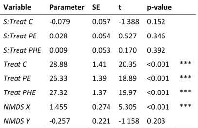
Table S4 Results from the mixed effects model for aboveground biomass TB with respect to species
richness S, exclusion treatment Treat (control C; predator exclusion PE; predator and herbivore exclusion PHE), and community composition represented by the first and second NMDS axes only (X and Y, respectively).
Variable Parameter SE t p-value
S:Treat C -0.079 0.057 -1.388 0.152 S:Treat PE 0.028 0.054 0.527 0.346 S:Treat PHE 0.009 0.053 0.170 0.392 Treat C 28.88 1.41 20.35 <0.001 *** Treat PE 26.33 1.39 18.89 <0.001 *** Treat PHE 27.32 1.37 19.97 <0.001 *** NMDS X 1.455 0.274 5.305 <0.001 *** NMDS Y -0.257 0.221 -1.158 0.203 ·P≤0.1, *P≤0.05, **P≤0.01, *** P≤0.001
Table S5 Results from the mixed effects model for aboveground biomass TB with respect to species
richness S, exclusion treatment Treat (control C; predator exclusion PE; predator and herbivore exclusion PHE), and plant species composition included as a random effect, expresses as a categorical variable based on sown species mixture with 37 levels.
Variable Parameter SE t p-value
S:Treat C -0.193 0.058 -3.333 0.001 *** S:Treat PE -0.036 0.056 -0.638 0.525 S:Treat PHE -0.092 0.053 -1.731 0.087 · Treat C 31.32 1.46 21.51 <0.001 *** Treat PE 27.81 1.46 19.02 <0.001 *** Treat PHE 29.73 1.38 21.62 <0.001 *** ·P≤0.1, *P≤0.05, **P≤0.01, *** P≤0.001
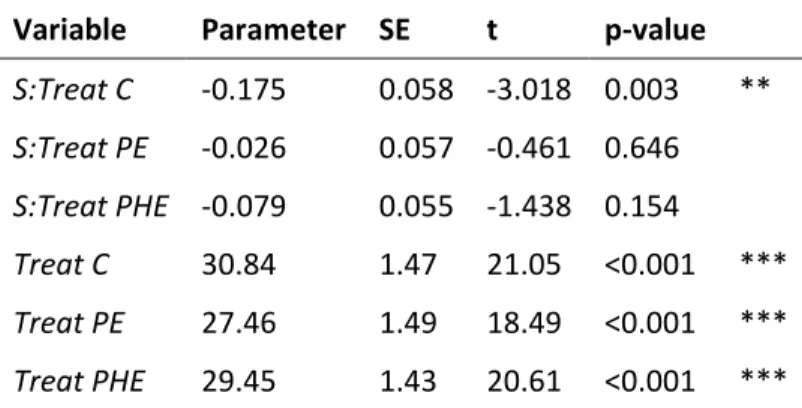
Table S6 Results from the mixed effects model for aboveground biomass TB with respect to species
richness S, exclusion treatment Treat (control C; predator exclusion PE; predator and herbivore exclusion PHE), and plant species composition included as a random effect, expressed as a categorical variable based on PAM clustering with 3 levels.
Variable Parameter SE t p-value
S:Treat C -0.175 0.058 -3.018 0.003 ** S:Treat PE -0.026 0.057 -0.461 0.646 S:Treat PHE -0.079 0.055 -1.438 0.154 Treat C 30.84 1.47 21.05 <0.001 *** Treat PE 27.46 1.49 18.49 <0.001 *** Treat PHE 29.45 1.43 20.61 <0.001 *** ·P≤0.1, *P≤0.05, **P≤0.01, *** P≤0.001
Table S7 Results from the mixed effects model for aboveground biomass TB with respect to species
richness S, exclusion treatment Treat (control C; predator exclusion PE; predator and herbivore exclusion PHE), and plant species composition included as correlation structure in the residuals (measured as a Jaccard similarity matrix). The p-value for the parameter λ was obtained by a log-likelihood ratio test for the model with vs. without plant composition as correlation structure.
Variable Parameter SE t p-value
S:Treat C -0.151 0.067 -2.277 0.030 * S:Treat PE -0.010 0.062 -0.169 0.393 S:Treat PHE -0.038 0.064 -0.589 0.334 Treat C 29.96 1.65 18.15 <0.001 *** Treat PE 26.67 1.62 16.43 <0.001 *** Treat PHE 27.65 1.62 17.10 <0.001 *** λ 0.795 <0.001 *** ·P≤0.1, *P≤0.05, **P≤0.01, *** P≤0.001
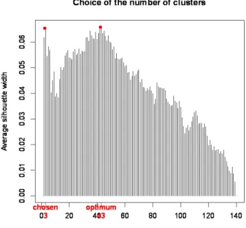
Figure S1 PAM clustering average silhouette width. The optimum clustering results in 43 clusters with
an average silhouette width of 0.0659. We chose the clustering with only 3 clusters. This point corresponds to the first maximum of the average silhouette width curve with a value of 0.0656.
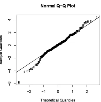
Figure S3 Q-Q plot of the residuals of the model with composition as NMDS axes
Figure S4 Q-Q plot of the residuals of the model with composition as random variables based on
Figure S5 Q-Q plot of the residuals of the model with composition as random variables based on
PAM clustering
Figure S6 Q-Q plot of the residuals of the model with composition as correlation in the residual