Practitioner’s Corner
Christian Kleiber* and Achim Zeileis
Reproducible Econometric Simulations
Abstract: Reproducibility of economic research hasattracted considerable attention in recent years. So far, the discussion has focused mainly on reproducibility of empirical analyses. This paper addresses a further aspect of reproducibility, the reproducibility of computational experiments. More specifically, we contribute to the emerg-ing literature on reproducibility in economics along three lines: (i) we document how simulations of various types are an integral part of publications in modern economet-rics, (ii) we provide some general guidelines about how to set up reproducible simulation experiments, and, finally, (iii) we provide a case study from time series econometrics that illustrates the main issues arising in connection with reproducibility, emphasizing the use of modular tools. Keyword: computational experiment; reproducibility; simulation; software.
*Corresponding author: Christian Kleiber, Universität Basel –
Faculty of Business and Economics, Peter Merian-Weg 6, 4002 Basel, Switzerland, E-mail: christian.kleiber@unibas.ch
Achim Zeileis: Faculty of Economics and Statistics, Universität
Innsbruck, Universitätsstr. 15, 6020 Innsbruck, Austria
1 Introduction
The issue of reproducibility of research in economics has attracted considerable attention in recent years. Publica-tions such as McCullough and Vinod (2003) demonstrate that in the absence of archives reproducibility is more an exception than the rule. Consequently, many leading economics journals recently introduced mandatory data archives, sometimes even mandatory code archives, coupled with corresponding editorial policies in order to provide sufficient information to facilitate replication. More recently, it has been found that even with archives there is no guarantee for reproducibility (e.g., McCullough, McGeary, and Harrison, 2008). One reason appears to be the lack of broadly accepted guidelines for what authors have to provide to ensure replicability.
Apart from a few exceptions, among them an early unpublished working paper by Koenker (1996), the discus-sion has focused mainly on reproducibility of empirical
work, i.e., of estimates and tests, or more broadly of tables and figures, in studies analyzing real-world data, often tacitly assuming that computations do not involve random elements. However, nowadays many papers in economet-rics – methodological as well as applied – and computa-tional economics make use of simulations. For these, rep-lication is usually even harder than for empirical analyses because there is typically neither code nor data but only a textual description of the simulation setup in the paper.
Making readable code available for such simulations is therefore crucial because it happens rather easily that not all tiny details of either the data-generating process (DGP) or the analysis methods are spelled out. Computer code is typically much more concise and less clumsy for specifying such details, e.g., the exact distribution of artificial data, the precise specification of a model or test employed, tuning parameters, etc.
This immediately raises the question of why we should want to be able to reproduce the results of econometric simulations. There would seem to be different reasons for different groups of people: In the publication process, the availability of replication materials can help to resolve questions regarding technical details and convince review-ers that the results are correct. (Of course, we can and do not expect that simulations are fully checked and repli-cated on a regular basis in the publication process.) On the production side, there are also direct incentives and tangi-ble benefits for the authors themselves: replication files for simulations should improve chances for acceptance of man-uscripts in the publication process and, ultimately, recep-tion of the work. Specifically, providing replicarecep-tion details will enhance communication of the underlying ideas and concepts to interested readers and hence improve under-standing of the associated results. Hence the availability of code should also facilitate follow-up work by other authors, such as applying different methods on the same DGPs, or evaluating the same methods on different DGPs.
In addition to the code, publication of the simulation results themselves (in the form of data) is often desirable. Regrettably, this is still not very common in economics and econometrics. Two notable exceptions from econo-metrics with impact on applied work involve nonstan-dard distributions in time series econometrics: Hansen (1997) and MacKinnon, Haug, and Michelis (1999) obtain
approximate asymptotic p values for certain structural change and cointegration tests, respectively, employing simulation techniques combined with response surface regressions. The simulation results are (or were: the archive of the Journal of Business and Economic Statistics no longer exists) available from the archives of the respec-tive journals.
Below we first, in Sections 2 and 3, examine recent volumes of two leading econometrics journals and docu-ment the types of computational experidocu-ments conducted in the field, their relative frequencies, the amount of detail available regarding the computational aspects, and the way of reporting the results. We find that current practice is quite uneven and that relevant details are often unavail-able. Very few papers are demonstrably replicable, in the sense that, in addition to any data, code for all simula-tion experiments is available. Since no set of generally accepted rules for computational experiments appears to be available in the econometrics literature, Section 4 next suggests some guidelines that might help to improve upon the current situation. These complement guide-lines for empirical work that were recently proposed by McCullough et al. (2008).
Perhaps the costs of better reporting are still seen as rather high, at least by some authors. However, given that authors typically have replication materials of their own simulations for themselves, the additional costs of preparing these for publication should be relatively small compared to the potential benefits, such as those out-lined above. Thus, in order to show that these costs are often lower than currently perceived, at least for some more standard tasks, we finally illustrate in Section 5 how modular tools for carrying out simulation studies could be made available. We employ such tools for replicating parts of Ploberger and Kr ä mer (1992), specifically a simulation of power comparisons for certain structural change tests.
2 Simulations in Econometrics
The importance of simulations in econometrics has increased considerably during the last 10 – 15 years. Hoaglin and Andrews (1975), in an early paper explor-ing then current practice in reportexplor-ing computation-based results in the statistical literature, found that the ratio of papers with simulation results to total papers was about one to five when examining then recent volumes of two statistics journals. More than 30 years later, the situa-tion has reversed: the ratio of papers without simulasitua-tion results to total papers is now less than one to five, as we shall see below. Also, 20 – 30 years ago simulations were
mainly used for performance comparisons of estimators and tests and also for evaluating nonstandard distribu-tions, whereas several recent techniques of statistical inference themselves contain stochastic elements.
2.1 Types of Simulations
In modern econometrics, simulations typically arise in one of the following forms:
– Monte Carlo studies.
These are usually employed for assessing the finite-sample power of tests or the performance of compet-ing estimators.
– Evaluation of nonstandard distributions.
As noted above, examples are found in time series econometrics, where many limiting distributions associated with unit root, cointegration or structural change methodology involve functionals of Brownian motion, for which tractable analytical forms are often unavailable.
– Resampling.
This typically means bootstrapping or subsampling, often in order to obtain improved standard errors, confidence intervals or tests. A less common tech-nique, at least in econometrics, is cross validation. – Simulation-based estimation.
This mainly refers to Bayesian and frequentist compu-tations employing Markov Chain Monte Carlo (MCMC) machinery, further methods include simulation-based extensions of the method of moments or of maximum likelihood.
There are further but currently less common variants such as heuristic optimization, often confined to specialized journals in operational research or statistics. Also, there is the rapidly expanding field of computational economics (as opposed to econometrics), notably agent-based mod-elling. Here we restrict ourselves to techniques typically found in econometrics.
2.2 Some Technical Aspects
Simulation methods require numbers that are or appear to be realizations of random variables, in the sense that they pass certain tests for randomness. “ Pseudorandom ” numbers are obtained using a random number genera-tor (RNG), typically a deterministic algorithm that recur-sively updates a sequence of numbers starting from a set of initial values called the “ (random) seed. ” (There also exist “ quasirandom ” numbers generated from a physical
device, but for reproducibility full understanding of the generation process is crucial, hence we shall confine our-selves to pseudorandom numbers.)
Random number generation typically proceeds in two steps: (i) generation of pseudorandom numbers resembling an independent and identically distributed (i.i.d.) stream from a uniform distribution on the interval (0,1), and (ii) transformation of this sequence to the required objects. If the latter are random numbers from a specific univariate distribution, the transformation being used is often the associated quantile function; the entire procedure is then referred to as the “ inversion method. ” However, some spe-cialized methods also exist for other distributions, notably the standard normal. It should further be noted that econo-metric computing environments often provide functions that directly deliver random numbers for many standard statistical distributions, hence the above steps may not be visible to the user. For step (i), a currently popular uniform RNG – used below for our own simulations – is the Mersenne twister (Matsumoto and Nishimura, 1998). Gentle (2003) provides useful general information on random number generation including algorithms, while Chambers (2008, Chapter 6.10) is geared towards R, the computing environment used in this paper.
One source for differences in simulation studies is differences in RNGs. Ideally, these differences should be small. However, this issue is likely to be relevant if truly large simulation studies are required as some older but still widely available RNGs might not be up to the task. Simulation studies should therefore always report the RNGs employed. A casual exploration of the econome-trics literature suggests that very few papers do so. We will come back to this issue below. In the supplements to this paper, we provide an example comparing simulation results obtained from two different RNGs.
Even if identical RNGs are used in the same com-puting environment, small differences will result from different initializations of the pseudo RNG, the random seeds. Hence papers reporting on simulations should also provide random seeds, at least in the code accompanying the paper. We shall see that this is highly uncommon in the journals we examined.
On a more technical level, some (typically tiny) dif-ferences can occur even when the same seed and RNG are used on different hardware architectures. The usual caveats concerning floating point arithmetic apply (see Goldberg, 1991).
As a straightforward robustness check, users could run the same experiment using (some combination of) different seeds, RNGs, operating systems and/or even dif-ferent machines.
3 Current Practice
For concreteness, we conducted a small survey in the fall of 2009 using the then most recent complete volumes of two econometrics journals. Specifically, we examined volume 23 (2008) of the Journal of Applied Econometrics (hereafter JAE) and volume 153 (2009) of the Journal of
Econometrics (hereafter JoE). The JAE is a journal with a
fairly comprehensive data archive. Since 1995, it requires authors to provide their data prior to publication (unless they are proprietary). The JoE is a journal with a more methodological bent. In contrast to the JAE, it currently does not have archives of any form. In our survey, we were interested in the variety of applications involving simula-tions and also in the amount of detail provided. The JAE volume 23 comprises seven issues containing 44 papers, including three software reviews and one editorial (per-taining to a special issue on the econometrics of auctions). Among the 40 remaining papers presenting empirical analyses, only seven do not contain any simulations, on average one paper per issue. Thus, a large majority of papers in the JAE makes use of simulations, with varying levels of complexity. In the JoE volume in question, com-prising two issues containing 15 papers in total, there is only a single paper not making use of simulations.
Table 1 details the frequencies of the various types of simulation studies listed in the preceding section, and also the amount of information provided. We see that the majority of papers in both journals makes use of simulation techniques, in one form or other. In Table 1 , simulation-based estimation often means some variant of MCMC, but there are also examples of the methods of simulated moments (MSM) or simulated scores (MSS). Resampling usually means some form of bootstrapping; one paper employs cross validation. With respect to the types listed above there are furthermore some clear differ-ences between the journals: in the JoE, the typical com-puter experiment is a Monte Carlo study, while in the JAE there is much greater variety. This presumably reflects the fact that new methodology, the dominant type of con-tribution in the JoE, by convention requires, apart from theoretical justification, some limited support employ-ing artificial data. It should also be noted that in the JAE the extent of computational experimentation is moreo-ver quite hetero geneous: Some simulation experiments amount to “ routine ” applications of, e.g., bootstrap stand-ard errors (this is the case for seven out of 15 JAE papers with resampling, but for none of the three papers from the JoE), others require a substantial amount of programming for novel algorithms or new implementations of (vari-ants of) existing ones. We found that papers employing
resampling techniques typically provide very little detail, although there are many variations of the bootstrap. These papers are thus among the least reproducible papers that are included in our study.
Evidence of lack of attention to computational detail is provided by the fact that only for 65.0% and 26.7% of the manuscripts, respectively, the computing environ-ment/programming language for all codes could be deter-mined. In the manuscripts that indicated the software environment(s), a variety of different tools was employed in both journals (numbers of occurrences in parentheses): GAUSS (12), Stata (7), MATLAB (6), Fortran (3), R (3), EViews (2), while Frontier, GLLAMM-STATA, Mathe-matica, PcGive, SAS, STABLE, SUBBOTOOLS, TRAMO/ SEATS, WinBUGS were each mentioned once. This already includes software that was not necessarily used for the simulations themselves but for some other computational task and also involves educated guessing by the authors based on implicit information.
Availability of the software was rarely mentioned. In the case of the JAE, code sometimes was nonetheless available from the archive, although this was not obvious from the paper; in some of these cases it even was con-tained in zipped files named “ data, ” so it was necessary to inspect the entire contents of the archives. It is also worth noting that papers using proprietary data often do not supply code, presumably because full replication is impossible under these circumstances. Among the papers that provide code, only six (combined for both journals) provide code with random seeds, for one further paper the corresponding README file explicitly states “ random draws are not seeded ” (!). (Note that we were liberal in
recording a paper as specifying the seeds; any partial specification was counted.) Only one code explicitly con-tains the RNG.
To summarize, the amount of available information required for replication is very heterogeneous: there are papers with very little information in the paper itself and no supplements of any kind, papers with fairly detailed descriptions of algorithms (but not necessarily of their implementation) but no code, papers with brief outlines but code available elsewhere [upon request, from a web page, in the archive of the journal (not always mentioned in the paper)]. Sometimes there is a reference to an earlier working paper with further details. Some authors also acknowledge reusing other people ’ s code in a footnote or the acknowledgements.
Finally, a striking difference between the JAE and the JoE is that although neither journal requires the authors to supply code, the journal with an archive (the JAE) none-theless succeeds in obtaining codes for some of its papers, because authors voluntarily deliver such files along with their data. In the case of the JoE, there is only a single paper (Moon and Schorfheide, 2009) for which codes are available from the web page of one of its authors.
Some preliminary conclusions from our survey would thus seem to be that (1) without archives there is little chance that relevant materials will become avai-lable, (2) voluntary or partial archives already represent a substantial improvement, and, in view of the amount of heterogeneity observed here, (3) some standardized rules for the precise form of the supplementary materials are needed. We shall expand on these issues in Sections 4 and 6 below.
Table 1 Summary of Simulation Survey for Journal of Applied Econometrics (JAE), Volume 23, and Journal of Econometrics (JoE), Volume 153. Note that the “ Data availability ” Categories are Mutually Exclusive While all Other Categories are Not. Proportions are Given in Percent.
JAE JoE
Frequencies of manuscripts In total 40 15
With simulation 33 14
Frequencies of data availability In archive 31 0
Proprietary 6 0
Not available 0 12
None used 3 3
Frequencies of simulation types Monte Carlo 17 11
Resampling 15 3
Simulation-based estimation 13 3
Nonstandard distributions 2 0
Proportion of all manuscripts With simulation 82.5 93.3
Indicating software used 65.0 26.7
Providing code 45.0 6.7
With code available upon request 17.5 0.0
Proportion of simulation manuscripts With replication files 30.3 7.1
4 Guidelines
Reproducibility of simulations, or more generally of com-putational experiments, has been a recurring theme in various branches of computational science. Examples of papers providing guidelines for statistics, engineering and applied mathematics (notably optimization) include Hoaglin and Andrews (1975); Crowder, Dembo, and Mulvey (1979); Jackson et al. (1991), Lee et al. (1993) and Barr et al. (1995). It should be noted that some of these works, namely those from the operational research litera-ture, are mainly concerned with performance compari-sons of algorithms, but many aspects are relevant here as well.
Similar guidelines in the context of econometric simulations are less common. A notable exception is the unpublished working paper of Koenker (1996) with its accompanying web page that provides a protocol for reproducible simulations in R, the computing environ-ment also used below. Drawing on the aforeenviron-mentioned works, we provide a checklist slightly adapted to the needs of econometrics.
In view of the diversity of tasks encountered in Section 3 it is not easy to provide detailed recommenda-tions that address all needs. However, we feel that the list below might give a good idea of what is required, espe-cially for more standardized tasks such as Monte Carlo studies.
We suggest that any paper presenting results from computational experiments should contain the following elements (or provide them as a supplement):
1. Description of the (statistical/econometric) model. 2. Technical information (software environment
including version numbers). 3. Code.
4. Replication files. 5. (Intermediate) results.
Some comments on the various elements are in order (further general comments follow below):
1. The paper should explain the methodology employed in reasonable detail. For specialized techniques requiring particularly lengthy descriptions, electronic supplements might be appropriate. Many journals now accept such supplements and publish them along with the papers.
2. As a vehicle for providing technical information such as software and version numbers we suggest to include, in the body of the paper, a section named ‘ computational details ’ such as the one appearing below. Currently, this information is often only
implicitly and approximately available; for example, because the computing environment is mentioned so that readers with access to the relevant software can find out more about RNGs etc.
3. Code typically means a collection of functions or macros, either provided by the authors themselves or by third parties. In our own replication study appearing in the following section it consists of Tables 2 – 4 and the strucchange package. If third-party code is used, it should be properly referenced. 4. The replication files themselves should contain the
exact function calls providing all tables and figures of the paper. Hence, they must always contain the random seed(s). If the software package offers several RNGs, the code should also be explicit regarding the chosen RNG. Compare the RNGkind() and set seed() calls in our example. In our case, Table 5 would serve as the replication file.
5. It is often useful to also provide the simulation results themselves in a file. As a rule, such data should be treated like any other data set, they supplement the paper and should thus be archived just like the data sets now required prior to publication of empirical work by many of the leading economics journals. In our case, a Monte Carlo study, the results are tables of simulation results, at a reasonable precision. In other types of simulation studies, other forms of (intermediate) results might be more relevant. For bootstrap exercises, this could mean saving sets of observation numbers. For MCMC jobs, saving a thinned version of the chain (say every 50th iteration, minus the burn-in phase) could be appropriate. The paper should explicitly state if supplements are avail-able, and if so where from. The preferred place for all supplements (code, results, further documentation, etc.) is the archive of the journal. For journals with only man-datory data archives we suggest that authors nonetheless also deposit code there (as we observed in several cases at the JAE). For journals still not possessing archives of any form, authors could provide materials on their personal web pages, or upon request. Clearly, a personal web page provides a much less permanent solution, and material “ available upon request ” typically even less so.
If simulation results are provided as data in supple-mentary files or data archives (such as our file sc_sim. csv), it would also remove the need to print all simula-tion results within the manuscript – the current prac-tice in econometrics. Instead, graphical displays (such as Figure 1 ) could be employed which are often more compact and thus more easily grasped than tables (such
as Table 6 ). In this case, replication code for producing the figures from the tables should be included in the supple-ments (see our Table 5).
In addition to the simulation results themselves, papers should also give information on their accuracy, e.g., in the form of standard errors. For many simulated probabilities (such as the power curves in Section 5) these are evident from the point estimates, however, more gene-rally they are not. Specifically, for many MCMC applica-tions, Flegal, Haran, and Jones (2008) suggest that there is room for improvement.
Regarding code it must also be taken into account that modern techniques are often highly nonlinear and thus inherently difficult to apply even outside the context of simulation studies. It is therefore mandatory to report tuning parameters, if any, along with the specification of the numerical algorithms themselves. For example, if a simulation involves use of iterative algorithms in an opti-mization problem, then the stopping criterion must be provided in some form, typically code.
Some aspects of the guidelines suggested above might prove difficult to meet if proprietary software is used for the simulations. As already noted by Jackson et al. (1991, p. 417) some 20 years ago, “ proprietary software presents special problems, ” in that it intentionally withholds certain details of the implementation from the user (or reader). In fact, as early as 1975 Hoaglin and Andrews (1975, p. 125) recommend using software in the public domain for precisely this reason. We remark that the current definition of “ public domain, ” at least in the US, is perhaps more restrictive than needed for the purpose of reproducibility. The authors feel that open source soft-ware might be sufficient.
5 Example: The Power of Structural
Change Tests
To illustrate the main issues in reproducibility of simu-lations we now replicate a Monte Carlo study from the methodological literature on tests for structural change. We have deliberately chosen a fairly simple (and success-ful) replication exercise in order to provide detailed infor-mation about all steps involved which in turn are helpful illustrations for the guidelines suggested in Section 4.
Ploberger and Kr ä mer (1992) compared their CUSUM test based on OLS residuals with the standard CUSUM test based on recursive residuals, showing that neither has power against orthogonal shifts. Here, we follow their simulation setup, but to make it a little more satisfying
methodologically (and cheaper to compute) we also compare the OLS-based CUSUM test to the Nyblom-Hansen test (Nyblom 1989; Nyblom-Hansen 1992) which in con-trast to the residual-based CUSUM tests is consistent for orthogonal changes.
The simulation setup considered by Ploberger and Kr ä mer (1992) is quite simple, and very clearly described. They consider a linear regression model with a constant and an alternating regressor x t = (1,( – 1) t ) ( t = 1, … , T ), inde-pendent standard normal errors, and a single shift in the regressor coefficients from β to β + Δ at time T * = z * T ,
z* ∈ (0,1). In the simulation, they vary the intensity b ,
the timing z * and the angle ψ of the shift as given by = /Δ b T( cos ,sin ),ψ ψ corresponding to their Equation 35. They give sequences of values for all three parame-ters and simulate power for a sample size of T = 120 from N = 1000 runs at the 5% significance level. This is a rather good description of the DGP, only two very small pieces of information are missing: β was left unspecified (presum-ably because the tests are invariant to it) and it is not com-pletely clear whether the observation T * (if it is an integer) belongs to the first or second regime. Given the design of their previous simulation in their Equations 33 and 34, one could speculate that it belongs to the second regime. However, we will place it in the first regime so that z * = 0.5 corresponds to two segments of equal size (for T even).
To turn their simulation design into modular and easily reusable code, we split it into three functions that capture the most important conceptual steps:
1. dgp() – the DGP that simulates a data set for a given scenario,
2. testpower() – a function that evaluates the tests on this DGP by power simulations,
3. simulation() – a wrapper function that runs a loop over all scenarios of interest using the previous two functions.
We implement these functions in the R system for statistical computing (R Development Core Team 2012), the source code is provided in Tables 2 , 3 , and 4 , respectively.
For step (1), function dgp() is a concise and easily accessible code description of the DGP described verbally above which can now be employed to apply the test pro-cedures of interest to artificial data resulting from dgp().
Based on this, we can define the function testpower() for step (2) that takes the number of replications and the size of the test as its main parameters. We provide functionality for evaluating the tests of interest, the OLS-based CUSUM test and the Nyblom-Hansen test, as well as the recursive CUSUM test considered by Ploberger and Kr ä mer (1992). All tests are available in the strucchange package (Zeileis
Table 3 Step (2) – Function testpower() for Evaluating Power Simulations of the Tests on a Single DGP Scenario generated by dgp() (see Table 2).
testpower < – function(nrep = 100, size = 0.05,
test = c("Rec–CUSUM", "OLS–CUSUM", "Nyblom–Hansen"),...) {
pval < – matrix(rep(NA, length(test) * nrep), ncol = length(test)) colnames(pval) < – test
for(i in 1:nrep) { dat < – dgp(...)
compute_pval < – function(test) {
test < – match.arg(test, c("Rec–CUSUM", "OLS–CUSUM", "Nyblom–Hansen")) switch(test,
"Rec–CUSUM" = sctest(y ~x, data = dat, type = "Rec–CUSUM") $ p.value,
"OLS–CUSUM" = sctest(y ~x, data = dat, type = "OLS–CUSUM") $ p.value,
"Nyblom–Hansen" = sctest(gefp(y ~x, data = dat, fit = lm),
functional = meanL2BB) $ p.value) }
pval[i,] < – sapply(test,compute_p val) }
return(colMeans(pval < size)) }
et al., 2002). 1 The function simply runs a loop of length
nrep, computes p values for the tests specified and finally computes the empirical power at level size. Furthermore, by using the ... notation in R all arguments used previ-ously for dgp() can simply be passed on.
In step (3), a wrapper function simulation() is defined that evaluates testpower() for all combina-tions of the simulation parameters, by default setting them to b = 0, 2.5, 5, 7.5, 10, z* = 0.25, 0.5, ψ = 0, 45, 90 for T = 100 and N = 100 using only the OLS-based CUSUM test and the Nyblom-Hansen test. This is a coarser grid as compared to Ploberger and Krämer (1992) with fewer replications which are sufficient for illustration here. The function
simulation() first expands the grid of all parameter combinations, then calls testpower() for each of them [which in turn calls dgp()] and then rearranges the data in a data frame.
Modular tools are extremely valuable when setting out to reproduce portions of a simulation study. They convey clearly what steps were carried out, the DGP could be reused for evaluating other structural change tests, or the tests could be reused on new DGPs. With these tools available, the main simulation amounts to loading the strucchange package, specifying the RNG, 2 setting a
random seed and executing simulation(), see Table 5 . 3
Table 2 Step (1) – Function dgp() for Generating a Data set from the Specified DGP.
dgp < – function(nobs = 100, angle = 0, intensity = 10, timing = 0.5, coef = c(0, 0), sd = 1)
{
angle < – angle * pi/180
delta < – intensity/sqrt(nobs) * c(cos(angle), sin(angle)) err < – rnorm(nobs, sd = sd)
x < – rep(c(–1, 1), length.out = nobs) y < – ifelse((1:nobs)/nobs < = timing, coef[1] + coef[2] * x + err,
(coef[1] + delta[1]) + (coef[2] + delta[2]) * x + err) return(data.frame(y = y, x = x))
}
1 The interface for the Nyblom-Hansen test is somewhat different
to avoid assessment of the stability of the error variance. Following Hansen (1992) this would be included by default, however, it is ex-cluded here for comparability with the residual-based CUSUM tests that do not encompass a test of the error variance.
2 Our call to the default RNG is identifiable as long as the version
number of the software is given. The version number appears in the “ Computational Details ” section at the end of this paper.
3 The parameters have been chosen such that the code can be run
interactively, possibly while grabbing a coffee (or another preferred beverage).
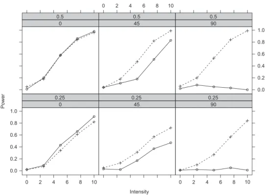
With a small simulation study as this one, we would generally only store the code and the outcome contained in sc_sim. For more complex simulations, it might make sense to store some intermediate results as well, e.g., the simulated data sets. Given the simu-lated results, it is easy for readers to replicate Table 6 . This compares the power curves (over columns corre-sponding to intensity) for the two tests (nested last in the rows) given angle and timing. Instead of inspect-ing this table, the differences between the two tests can be brought out even more clearly graphically in a trellis (or lattice) type layout such as Figure 1 , using the same nesting structure as above. The replication code for tabular and graphical summary is also included in Table 5 , employing the lattice package (Sarkar 2008) for visualization.
Table 6 Simulated Size and Power for OLS-Based CUSUM Test and Nyblom-Hansen Test.
Angle Timing Test Intensity
0 2.5 5 7.5 10 0 0.25 OLS-CUSUM 0.02 0.09 0.43 0.66 0.91 Nyblom-Hansen 0.02 0.07 0.34 0.61 0.82 0.5 OLS-CUSUM 0.01 0.20 0.58 0.86 0.98 Nyblom-Hansen 0.05 0.18 0.58 0.84 0.96 45 0.25 OLS-CUSUM 0.03 0.02 0.17 0.37 0.47 Nyblom-Hansen 0.05 0.13 0.31 0.57 0.72 0.5 OLS-CUSUM 0.04 0.11 0.18 0.51 0.83 Nyblom-Hansen 0.04 0.18 0.47 0.82 0.99 90 0.25 OLS-CUSUM 0.01 0.02 0.01 0.05 0.01 Nyblom-Hansen 0.01 0.10 0.27 0.57 0.84 0.5 OLS-CUSUM 0.02 0.08 0.05 0.03 0.00 Nyblom-Hansen 0.06 0.20 0.53 0.84 0.99 Table 4 Step (3) – Function simulation() for Looping over a Range of Scenarios Generated by dgp() (see Table 2) and Evaluated by testpower() (see Table 3).
simulation < – function(intensity = seq(from = 0, to = 10, by = 2.5), timing = c(0.25, 0.5), angle = c(0, 45, 90),
test = c("OLS–CUSUM", "Nyblom–Hansen"), ...) {
prs < – expand.grid(intensity = intensity, timing = timing, angle = angle) nprs < – nrow(prs)
ntest < – length(test)
pow < – matrix(rep(NA, ntest * nprs), ncol = ntest)
for(i in 1:nprs) pow[i,] < – testpower(test = test, intensity =
prs $ intensity[i], timing = prs $ timing[i], angle = prs $ angle[i], ...)
rval < – data.frame()
for(i in 1:ntest) rval < – rbind(rval, prs) rval $ test < – gl(ntest, nprs, labels = test) rval $ power < – as.vector(pow)
rval $ timing < – factor(rval $ timing) rval $ angle < – factor(rval $ angle) return(rval)
}
Table 5 Replication Code for Simulation Results Presented in Table 6 and Figure 1, Respectively. It Assumes that the Functions from Tables 2 – 4 are Loaded, then First Produces the Simulation Results, followed by the Replication of Tabular and Graphical Output.
library("strucchange")
RNGkind(kind = "default", normal.kind = "default") set.seed(1090)
sc_sim < – simulation()
tab < – xtabs(power ~ intensity + test + angle + timing, data = sc_sim)
ftable(tab, row.vars = c("angle", "timing", "test"), col.vars = "intensity")
library("lattice")
xyplot(power ~ intensity | angle + timing, groups = ~ test,
This shows rather clearly that only for shifts in the intercept (i.e., angle 0), the OLS-based CUSUM test per-forms very slightly better than the Nyblom-Hansen test, but dramatically loses power with increasing angle, being completely insensitive to orthogonal changes in slope only (i.e., angle 90). The Nyblom-Hansen test, however, performs similarly for all angles. Breaks in the middle of the sampling period are easier to detect for both tests. 4 All
results are roughly consistent with Table II(b) in Ploberger and Kr ä mer (1992) although we have reduced many of the parameter values for the sake of obtaining an almost inter-active example.
In the supplementary material to this article, we explore several variations of this simulation setup. In par-ticular, we investigate the following:
1. Running the simulation with the same parameters as Ploberger and Kr ä mer (1992), i.e., simulation (nobs = 120, nrep = 1000, intensity = seq(4.8, 1 2 , b y = 2 . 4 ) , t i m i n g = s e q ( 0 . 1 , 0 . 9 , by = 0.2),angle = seq(0, 90, by = 18), test = c (" Rec-CUSUM", "OLS-CUSUM")).
2. Increasing the number of replications to nrep = 100000 to obtain more precise power estimates.
3. Changing the random number generator for normal random numbers. The default used above is to employ the Mersenne Twister for generating uniform random numbers and then apply the inversion method. An alternative would be one of the many generators specifically designed for providing standard normal data such as the Kinderman-Ramage generator. In R this is used by setting RNGkind(normal.kind = "Kinderman-Ramage").
Unsurprisingly, the results are never exactly identi-cal, but fortunately all very similar. More precisely, we compute point-wise asymptotic 95% confidence intervals for the difference of simulated powers. The empirical coverage proportions for zero are: 95.0% for the pairwise differences of (1) and (2), 93.6% for the pairwise differences of (2) and (3), and 90.8% for the pairwise differences of (1) and the original table in Ploberger and Kr ä mer (1992). Hence, the agreement between the results is always fairly large. Only the origi-nal study deviates somewhat, but it still leads to quali-tatively equivalent conclusions. In the supplements to this paper, the exact simulation results are provided along with replication files.
4 These findings are not simply artefacts of using N = 100
replica-tions. The results from a larger, N = 10,000, experiment that we con-ducted reveal them even more clearly and additionally show that the OLS-based CUSUM test is somewhat conservative while the Nyblom-Hansen test is not.
Intensity Power 0.0 0.2 0.4 0.6 0.8 1.0 0 0.25 45 0.25 90 0.25 0 0.5 0 2 4 6 8 10 0 2 4 6 8 10 0 2 4 6 8 10 45 0.5 0.0 0.2 0.4 0.6 0.8 1.0 90 0.5
6 Conclusions
Scientific progress depends on the possibility to verify or falsify results. In the case of computer experiments in econometrics, verification or falsification of results is currently virtually impossible because the available infor-mation on computational detail in such experiments is often insufficient. To improve this unfortunate situation, a combination of measures is likely necessary: As a first step, authors need to be informed about requirements for reproducibility, i.e., availability of replication code along with results of the experiments. As a second step, jour-nals need to support this by providing archives for code in addition to data. Ideally, these archives are integrated into the editorial process so that their content is checked and well arranged. We hope that the guidelines presented above will be useful in implementing such measures.
It should also be borne in mind that users are responsible for their tools. Thus, in addition to the docu-mentation issues, some attention to the quality of the com-putational tools is advisable. It is worth noting that there are still many inferior RNGs around, or poor implementa-tions, even in widely used software packages. Ripley (1990) and Hellekalek (1998) are (still) useful starting points for the main issues. A more recent source is L ’ Ecuyer (2006). Users of simulation software should therefore consult the relevant software reviews. In econometrics, the JAE pub-lishes such reviews, in statistics, Computational Statistics
& Data Analysis (CSDA) is one of the journals that do.
Traditionally, the branch of statistics known as experi-mental design has received limited attention in economet-rics, presumably because in the social sciences true exper-iments are more an exception than the rule. However, computer experiments can, and should, be treated just like experiments typically associated with the hard sci-ences, hence the principles of experimental design apply. Not surprisingly, the statistical literature offers a number
of suggestions regarding the design of computational experiments, see e.g., Santner, Williams, and Notz (2003).
Quite apart from the main topic of this paper, a further important lesson appears to emerge from a comparison of the two journals we examined: some 30% of the JAE papers have supplements including (some) codes, although the JAE archive currently only requires submission of data. This is rather encouraging and suggests that even partial (in the sense of data-only) archives sometimes succeed in collecting crucial supplementary materials. Nonetheless, given that only one paper out of an entire volume of the JoE provides complete details on simulations a much higher compliance rate is needed, and hence our findings would seem to reiterate the need for code archives in addition to the recently adopted data archives. For further elabora-tion on the benefits of data and code archives we refer to to Anderson et al. (2008) and the references therein.
7 Computational Details
Our results were obtained using R 2.15.0 – with the pack-ages strucchange 1.4-6, and lattice 0.20-6 – and were identical on various platforms including PCs running Debian GNU/Linux (with a 3.2.0-1-amd64 kernel) and Mac OS X, version 10.6.8. Normal random variables were gen-erated from uniform random numbers obtained by the Mersenne Twister – currently R ’ s default generator – by means of the inversion method. The random seed and further technical details are available in the code supple-menting this paper.
Acknowledgments: We are grateful to Roger Koenker for feedback and discussion – part of this manuscript origi-nated in the work on Koenker and Zeileis (2009).
Previously published online March 15, 2013
References
Anderson, R.D., W. H. Greene, Bruce D. McCullough, and H. D. Vinod. 2008. “ The Role of Data/Code Archives in the Future of Economic Research. ” Journal of Economic Methodology 15: 99 – 119. Barr, R.D., B. L. Golden, J. P. Kelly, M. G. C. Resende, and W. R.
Stewart, Jr. 1995. “ Designing and Reporting on Computational Experiments with Heuristic Methods. ” Journal of Heuristics 1: 9 – 32.
Crowder, H., R. S. Dembo, and J. M. Mulvey. 1979. “ On Reporting Computational Experiments with Mathematical Software. ” ACM
Transactions on Mathematical Software 5 (2): 193 – 203.
Flegal, J. M., M. Haran, and G. L. Jones. 2008. “ Markov Chain Monte Carlo: Can we Trust the Third Significant Figure? ” Statistical
Science 23 (2): 250 – 260.
Gentle, J. E. 2003. Random Number Generation and Monte Carlo
Methods . 2nd ed. New York: Springer-Verlag.
Hansen, B. E. 1992. “ Testing for Parameter Instability in Linear Models. ” Journal of Policy Modeling 14: 517 – 533. Hansen, B. E. 1997. “ Approximate Asymptotic p values for
Structural-Change Tests. ” Journal of Business & Economic
Hellekalek, P. 1998. “ Good Random Number Generators are (not so) Easy to Find. ” Mathematics and Computers in Simulation 46: 485 – 505.
Hoaglin, D. C., and D. F. Andrews. 1975. “ The Reporting of Computation-Based Results in Statistics. ” The American
Statistician 29: 122 – 126.
Jackson, R. H. F., P. T. Boggs, S. G. Nash, and S. Powell. 1991. “ Guidelines for Reporting Results of Computational
Experiments. Report of the Ad Hoc Committee. ” Mathematical
Programming 49: 413 – 425.
Koenker, R. 1996. “ Reproducible Econometric Research. ”
Working paper , Econometrics Lab, University of Illinois at Urbana-Champaign. http://www.econ.uiuc.edu/~roger/repro.html. Koenker, R., and A. Zeileis. 2009. “ On Reproducible Econometric
Research. ” Journal of Applied Econometrics 24: 833 – 847. L ’ Ecuyer, P. 2006. “ Random Number Generation. ” In Handbooks
in Operations Research and Management Science, Vol. 13: Simulation , edited by S. G. Henderson and B. L. Nelson, 55 – 81.
North-Holland, Amsterdam: Elsevier.
Lee, C.-Y., J. Bard, M. Pinedo, and W. E. Wilhelm. 1993. “ Guidelines for Reporting Computational Results in IIE Transactions . ” IIE Transactions 25 (6): 1 – 26.
MacKinnon, J. G., A. A. Haug, and L. Michelis. 1999. “ Numerical Distribution Functions of Likelihood Ratio Tests for Cointe-gration. ” Journal of Applied Econometrics 14: 563 – 577. Matsumoto, M., and T. Nishimura. 1998. “ Mersenne Twister: A
623-Dimensionally Equidistributed Uniform Pseudo-Random Number Generator. ” ACM Transactions on Modeling and
Computer Simulation 8 (1): 3 – 30.
McCullough, B. D., and H. D. Vinod. 2003. “ Verifying the Solution from a Nonlinear Solver: A Case Study. ” American Economic
Review 93: 873 – 892.
McCullough, B. D., K. A. McGeary, and T. D. Harrison. 2008. “ Do Economics Journal Archives Promote Replicable Research? ” Canadian Journal of Economics 41 (4): 1406 – 1420.
Moon, H. R., and F. Schorfheide. 2009. “ Estimation with Overiden-tifying Inequality Moment Conditions. ” Journal of Econometrics 153: 136 – 154.
Nyblom, J. 1989. “ Testing for the Constancy of Parameters Over Time. ” Journal of the American Statistical Association 84: 223 – 230. Ploberger, W., and W. Kr ä mer. 1992. “ The CUSUM Test with OLS
Residuals. ” Econometrica 60 (2): 271 – 285.
R Development Core Team.2012. R: A Language and Environment for
Statistical Computing . R Foundation for Statistical Computing,
Vienna, Austria, 2012. ISBN 3-900051-07-0. http://www.R-project.org/.
Ripley, B. D. 1990. “ Thoughts on Pseudorandom Number Generators. ” Journal of Computational and Applied
Mathematics 31: 153 – 163.
Santner, T. J., B. J. Williams, and W. I. Notz. 2003. The Design
and Analysis of Computer Experiments . New York:
Springer-Verlag.
Sarkar, D. 2008. lattice: Multivariate Data Visualization with R . New York: Springer-Verlag.
Zeileis, A., F. Leisch, K. Hornik, and C. Kleiber. 2002. “ strucchange: An R Package for Testing for Structural Change in Linear Regression Models. ” Journal of Statistical Software 7 (2): 1 – 38. http://www.jstatsoft.org/v07/i02/.