Re
search Article
Miriam Záme˘cníková*, Andreas Wieser, Helmut Woschitz, and Camillo Ressl
Influence of surface reflectivity on reflectorless
electronic distance measurement and terrestrial
laser scanning
Abstract: The uncertainty of electronic distance
mea-surement to surfaces rather than to dedicated precision-reflectors (reflectorless EDM) is affected by the entire sys-tem comprising instrument, atmosphere and surface. The impact of the latter is significant for applications like geodetic monitoring, high-precision surface modelling or laser scanner self-calibration. Nevertheless, it has not yet received sufficient attention and is not well understood. We have carried out an experimental investigation of the impact of surface reflectivity on the distance measure-ments of a terrestrial laser scanner. The investigation helps to clarify (i) whether variations of reflectivity cause system-atic deviations of reflectorless EDM, and (ii) if so, whether it is possible and worth modelling these deviations. The results show that differences in reflectivity may actually cause systematic deviations of a few mm with diffusely re-flecting surfaces and even more with directionally reflect-ing ones. Usreflect-ing a bivariate quadratic polynomial we were able to approximate these deviations as a function of mea-sured distance and meamea-sured signal strength alone. Using this approximation to predict corrections, the deviations of the measurements could be reduced by about 70% in our experiment. We conclude that there is a systematic ef-fect of surface reflectivity (or equivalently received signal strength) on the distance measurement and that it is pos-sible to model and predict this effect. Integration into laser scanner calibration models may be beneficial for high-precision applications. The results may apply to a broad range of instruments, not only to the specific laser scan-ner used herein.
*Corresponding Author: Miriam Záme˘cníková: Department of Geodesy and Geoinformation, Vienna University of Technology, Austria, E-mail: [email protected]
Andreas Wieser: Institute of Geodesy and Photogrammetry, ETH Zürich, Switzerland
Helmut Woschitz: Institute of Engineering Geodesy and Measure-ment Systems, Graz University of Technology, Austria
Camillo Ressl: Department of Geodesy and Geoinformation, Vienna University of Technology, Austria
Keywords: Laser scanning, EDM, Signal strength,
Calibra-tion, Error modelling
DOI 10.1515/jag-2014-0016
Received August 08, 2014; accepted October 03, 2014
1 Introduction
The uncertainty of electronic distance measurement (EDM) to dedicated reflectors like corner-cube prisms is well understood. The offset, scale factor and - in case of phase-based measurement principle - cyclic deviations can be determined by calibration of the measurement sys-tem. The accuracy of reflector-based EDM is then typically a function of distance and can be predicted very well. For distances longer than a few hundred meters it is practically limited by insufficient knowledge of the refractive index along the line-of-sight.
Laser scanners use the same basic principles for dis-tance measurement and are thus also subject to bias, scale deviation, distance dependent noise, possibly cyclic devi-ations, and variations of the refractive index. However, like other reflectorless (RL) EDM instruments, laser scanners derive the distance from signals reflected by the scanned surfaces themselves not by dedicated reflectors. This adds several degrees of freedom to the uncertainty budget be-cause the distance deviations now depend additionally on the surface and subsurface material, surface rough-ness, angle of incidence, energy distribution within the footprint, and on the resulting surface penetration and re-flectance. Previous studies have indicated that these ef-fects can cause systematic deviations of several mm or more; see e.g. [1, 2, 6, 7, 12–14]. The data sheets of re-lated instruments typically cite the RL-EDM accuracy for orthogonal measurement onto a homogeneous planar sur-face with a specific grey value and are therefore of very lim-ited practical use. The accuracy of RL-EDM is in fact more
often limited by the insufficient knowledge of the above surface parameters and their effect on the measured dis-tance than by that of the refractive index.
Nevertheless, there are only few systematic studies of the impact of reflectance, and proposals for calibration of terrestrial laser scanners (TLS) do not yet include a depen-dence of distance deviations on reflectance or on received signal strength, see e.g., [3, 5, 10]. This is likely due to the fact that the impact may be small and hidden within the noise of individual scanned points unless exposed by test on special facilities. However, in view of increasing preci-sion of the instruments and of noise reduction by spatial filtering (e.g., fitting surfaces to scanned point clouds) we consider a corresponding study relevant. Its results may become useful for scanner calibration in particular with respect to the cyclic deviations caused by interference be-tween the measurement signal associated with the target and spurious signals within the instrument [11]. The rela-tive power of the measurement signal with respect to the other ones is a main factor determining these cyclic devi-ations. This relative power is only a function of target dis-tance for a given prism and instrument with conventional EDM, but it is also a function of target reflectance in case of RL-EDM suggesting that reflectance or received signal strength should be input quantities in laser scanner error models.
We present an experimental investigation of the im-pact of surface reflectivity on the distance measurements of a phase-based terrestrial laser scanner Z+F IMAGER 5006i over distances up to 30 m. Using this investigation, we try to answer the following questions: (i) Do varia-tions in surface reflectivities cause systematic deviavaria-tions of phase-based RL-EDM? (ii) If they do, is it possible and worth modelling these deviations such that the accuracy of the raw measurements can be improved by applying the model?
Taking special precautions, which will be explained later, the results refer almost exclusively to the EDM com-ponent of the scanner, not to the angular measurements or to the mechanical components. Therefore, the results are qualitatively representative for the phase-based meas-urement principle and apply to a broad range of RL-EDM instruments, not only to the specific instrument used herein. The paper is intended to raise awareness of the im-pact of reflectivity on RL-EDM and TLS measurements, to enhance our understanding of systematic and random ef-fects, and to form the basis for a practically relevant exten-sion of the additional parameters (AP) proposed for TLS calibration by [5] and used by various authors since then. For most scanners, the transmission power is con-stant except for potential minor variations due instrument
warm-up or aging of components. So, the received signal strength of a given instrument is a function of distance and of the ratio between incident power and power reflected towards the instrument at the illuminated surface. This ra-tio, the reflectance, depends on the illuminated material, the thickness of the material in relation to the effective penetration depth, on the angle of incidence of the mea-surement beam onto the surface, and on surface rough-ness at scales exceeding the wavelength of the measure-ment beam. The upper bound of the reflectance, the so-called reflectivity is a material property [8]. Despite these definitions, we will use the term surface reflectivity in-stead of reflectance herein to indicate the relative power reflected towards the instrument from the direction of the
surface element illuminated by the footprint of the
mea-surement beam. This will be justified because we will use thick, smooth, homogeneous targets measured orthogo-nally and thus the observed reflectance will be equal to the reflectivity; impacts of surface roughness or angle of inci-dence will not be analyzed herein.
2 Methods
The experimental investigation is based on the compari-son of distances measured using TLS and corresponding distances measured using a laser interferometer. The lat-ter are several orders of magnitude more accurate than the TLS measurements, and the differences represent the true deviations of the TLS measurements which we want to study.
The chosen experimental setup is similar to the one used by other authors for the investigation of distance de-pendent effects on TLS measurements, see e.g. [12, 13], and traditionally used for determining the cyclic deviation of a conventional EDM instrument on a test line [4, 11]. How-ever, several special precautions were necessary to ensure sufficiently accurate reference values despite the use of dif-ferent surfaces as targets. The setup and these precautions will be presented in section 3.
The laser scanner was operated in 2D profile mode during this investigation. As compared to operation with fixed measurement beam (like with a conventional EDM) this gave us various options to study the stability and qual-ity of the data and the homogenequal-ity of the target surfaces while still keeping measurement time low enough to fa-cilitate the investigation. Data processing consisted of (i) the extraction of representative measurements from the profiles (i.e., measurements comparable to the interfer-ometer measurements), (ii) filtering of the measurements
to reduce random noise and better expose systematic ef-fects, (iii) application of geometrical corrections account-ing for changes due to target replacement and target non-planarity, and (iv) visual and numeric analysis of the dis-tance differences as a function of disdis-tance and received signal strength. The preparatory steps (i)-(iii) will be ex-plained in section 4. The analysis and discussion of the re-sults are given in section 5.
3 Experimental setup and
measurement process
3.1 Configuration
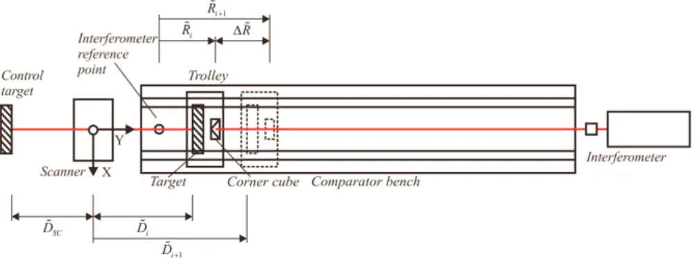
A laser scanner is setup at one end of a horizontal com-parator bench, an interferometer at the other one. A trolley which can be moved linearly along the comparator bench carries a flat target for the TLS measurements and a cor-ner cube prism for the interferometer measurements. The arrangement is shown schematically in Figure 1. The trol-ley is moved stepwise from the near end (i.e., minimum distance¹ ˜Dminbetween scanner and target) to the far end
of the comparator bench with fixed step size ∆ ˜R. At each
position ˜Riof the trolley, the interferometer measurement
Riand laser scanner profile measurements θk,i,land Dk,i,l
are recorded where θ is the vertical angle, D the distance,
k indicates the target, and l the measurement within the
2D-profile.
Targets with different reflectivity are used (see sec. 3.2) one at a time. The measurements are carried out in
cy-cles comprising a forward leg (near end to far end) and a backward leg (far end to near end) with one target. After
a cycle, the target is replaced and the measurements are repeated with a different one. For control purposes addi-tional legs are measured with some targets, and some cy-cles were repeated after target replacement. A fixed control target is mounted rigidly on a wall behind the scanner and included in all profile measurements for stability checking during and across the cycles.
For the later analysis the one-dimensional interferom-eter measurements should indicate precisely the true dis-tance differences ˜Dk1,i1− ˜Dk2,i2between any two targets k1
and k2and target positions i1and i2. Additionally, the an-gle of incidence of the laser beams onto the target surface should be the same for all targets, cycles and distances,
1 Throughout the paper the tilde symbol indicates true values as op-posed to measured ones.
and the measurements should always refer to the same lo-cation at the target surface. This requires meeting the fol-lowing conditions with sufficient accuracy (see also Fig-ure 2):
(C1) The comparator longitudinal axis BB is a straight line. (C2) The trajectory of any individual point of the trolley is parallel to BB when the trolley is moved along the comparator.
(C3)The measurement beam II of the interferometer is par-allel to BB.
(C4)A vertical angle ˜θrexists in the scanner coordinate
sys-tem such that the corresponding laser measurement beam MM is parallel to BB.
(C5) The target surface is perpendicular to MM.
(C6)The perpendicular distance ˜∆MIbetween MM and II is
small.
These conditions imply that the measurements need to be carried out in a controlled (lab) environment and that all components are set up and adjusted carefully. The corre-sponding steps will be briefly summarized in sec. 3.3.
3.2 Targets
Eight different planar targets were used for the measure-ments and the analysis presented herein, one of them as control target. All targets were of identical size (approxi-mately 13×13 cm2) and rigidly mounted on their own metal support which could in turn be inserted into a custom made holder attached to the trolley (see Figure 3). Table 1 gives the main characteristics of these targets.
Spectralon is a material with almost ideal Lambertian reflection and constant reflectance over the optical wave-lengths from 250 to 2500 nm². It is available in pure form or doped with black pigment for nominal reflectance values between 2% and 99%. The values indicate that the respec-tive target reflects the corresponding percentage of the en-ergy which a perfectly Lambertian material would reflect to the detector under the same illumination. Spectralon is well suited for radiometric tests and calibration.
Additionally, we have built targets of the same size affixing smooth cardboard to flat aluminum plates. We
2 Technical Guide: Reflectance Materials and Coatings. Labsphere, http://www.labsphere.com, accessed on July 15, 2014.
Fig. 1. Basic measurement setup (top view, not to scale).
Fig. 2. Geometrical relations within measurement setup (side view, not to scale; control target omitted).
Table 1. Targets used in the experimental investigation.
ID Reflectance† Material Comment
S99 99 % Spectralon
S80 87 % Spectralon
S40 47 % Spectralon control target (see Figure 1)
S05 7 % Spectralon
KaH 102 % white cardboard
KaG 81 % grey cardboard
KaS 10 % black cardboard
MeW 650 % aluminum thinly painted mat white
†Empirical values calculated from nominal reflectance of S99 and measured signal strengths using all profile measurements of the test described herein.
have selected materials which yielded approximately the same received signal strength at the laser scanner as the Spectralon targets S99, S80 and S05. Their reflectance at the wavelength of the chosen laser scanner was therefore nearly identical to the one of the Spectralon targets. So we had pairs of targets with equal reflectivity but made of different materials which would later allow distinguishing between effects due to reflectivity and effects due to mate-rial. Furthermore, cardboard is easily available and used by some laser scanner manufacturers to test their instru-ments.
Finally, we also built a highly reflective target from a flat aluminum plate thinly painted mat white. This target (MeW) was included to yield results associated with very high signal strengths. Actually, the later measurements showed that the signal strength received by the scanner at any given distance was more than 6 times higher using MeW than using S99 (see also Table 1). So, clearly this tar-get caused strong directional reflection as opposed to all other targets.
3.3 Adjustment of components
The measurements were carried out using the 30 m long comparator bench in the geodetic measurement labora-tory of the Graz University of Technology. From separate control measurements and adjustment of the bench it is known that the trolley experiences vertical and lateral de-viations from a straight line less than 0.4 mm when moving along the bench, with pitch, roll, and yaw variations less than 0.03 gon. Thus, when taking the size of the TLS foot-print into account (about 3 mm at the shortest distance), conditions C1 and C2 are sufficiently fulfilled by this com-parator without any further precautions.
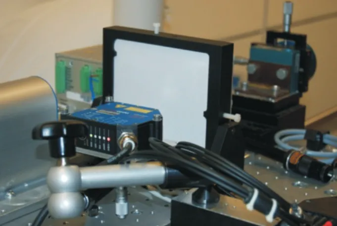
The corner cube and the target holder were rigidly mounted at the trolley such that their respective centers were offset longitudinally by about 32 cm, and less than 2 mm laterally and vertically. Then, the interferometer was set up using standard procedures such that condition C3 was fulfilled.
Using autocollimation mirrors, temporarily mounted on the target holder, and various auxiliary components the target holder was aligned such that the target surface was orthogonal to the interferometer axis II with devia-tions less than 0.001 gon at the near end position of the trolley. Using autocollimation and a level the laser scan-ner (mounted on an industrial tripod) was precisely posi-tioned and horizontally aligned at one end of the bench such that its trunnion axis was at approximately the same height as the target center. With these steps, conditions C4
Fig. 3. Target KaH on trolley (center); triangulation sensor temporari-ly set up for checking target adjustment (foreground).
to C6 were fulfilled, although the numerical values of ˜θr
and ˜∆MIwere not yet known.
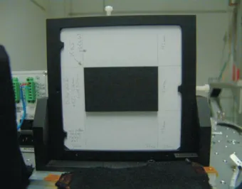
Finally, a special target with a dark rectangular card-board on a white background was mounted in the target holder (see Figure 4) and used to determine ˜θrfrom laser
scanner profile measurements with the trolley moved from the near end to the far one. The vertical angles correspond-ing to the respective black/white transitions could easily be identified in the signal strength profiles, and ˜θrwas
es-timated as the vertical angle which corresponded to the same location on the target plane (i.e., to the same relative position between the upper and lower black/white transi-tions) for all target distances. This location was very close to II (with ˜∆MI≈ 2 mm) because of the above scanner setup
using a level, and ˜θrwas close to 100 gon³.
3.4 Measurement process
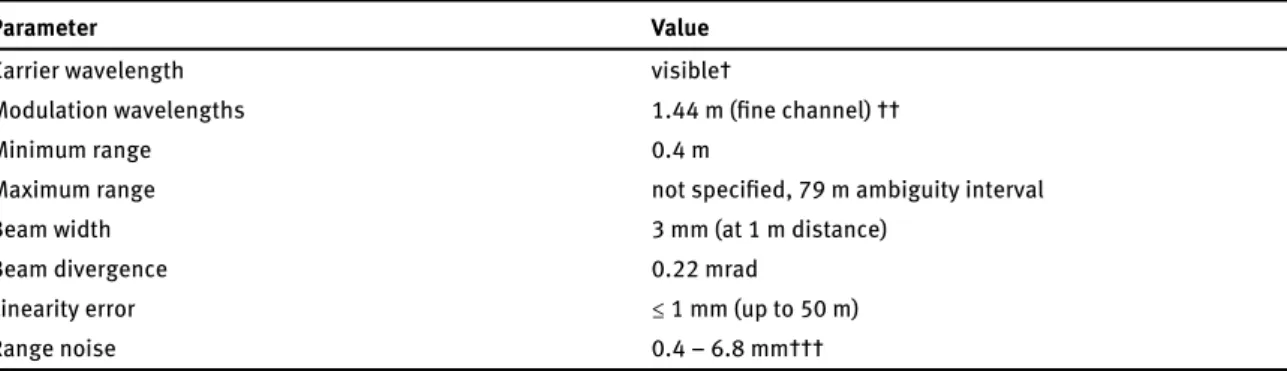
The entire measurement process except setup and target exchange was fully automated. The motorized trolley, the interferometer and the laser scanner were connected to a PC controlling the measurement process and recording the data. Due to availability, a phase-based scanner Z+F IM-AGER 5006i was used for the measurements (see Table 2). It had been with the manufacturer for maintenance and calibration shortly before, and all numeric results subse-quently obtained refer to measurements already corrected by the scanner software using the models implemented by
3 The deviation from 100 gon is irrelevant here. The angle would only be exactly 100 gon, if the scanner had no index offset and its Z−axis were perfectly orthogonal to the horizontal comparator longitudinal axis.
Fig. 4. Special target with black area on white background used during scanner setup.
the manufacturer. These models and details regarding cal-ibration are not disclosed and thus unknown to the au-thors.
During each measurement cycle, the trolley was moved from Dmin = 1.1 m to Dmax = 29.7 m and back
in steps of size ˜R = 7.5 cm. We had chosen this step size
in order to resolve even higher order harmonics in case there are significant cyclic deviations [11], given the EDM modulation wavelength of the fine channel of this scanner (see Table 2). The maximum distance was restricted by the available length of the comparator bench.
While the interferometer necessarily measured with-out interruption the laser scanner profile measurements were stopped before each target repositioning and started again after the target had reached its next position (as controlled by the interferometer). At each target position,
N = 300 profiles were measured and stored by the
scan-ner (12.5 rot/s, scan resolution of ∆θ= 0.018○, measure-ment time of 24 s) without rotation about its nearly ver-tical Z-axis. The number of profiles was chosen after first tests as a compromise between (i) high redundancy to fa-cilitate checking the temporal stability and calculating key statistical properties of the measurements, and (ii) keep-ing the time per measurement cycle within a manageable limit. Each cycle took about 10 hours.
The raw interferometer measurements Riare actually
observations of the true 1D displacements ˜Rifrom an
ar-bitrarily chosen reference point (see Figure 2). To assure that this reference point would be stable throughout the data collection and could be recovered in case of interrup-tion of the laser beam, inductive displacement transducers
were used for independently measuring the position of the trolley at its near end position with very high accuracy.
In order to verify that also the scanner – and thus the distance ˜LSIbetween the scanner and the interferometer –
remained stable, the profile measurements to the control target (see Figure 1) were analyzed. The measurements in-dicated that the distance ˜DSC between the control target
and the scanner actually remained constant within about 0.1 mm throughout the data collection process.
A critical step within this investigation was the re-placement of the targets. The true distance between the scanner and the targets cannot be measured using the cho-sen setup, only the target displacements along the line BB can be measured precisely. Using the above precautions it was possible to also measure trolley displacement dur-ing target exchange or across times when the interferome-ter beam had been ininterferome-terrupted. In order to relate all target measurements to a common reference position, the vari-ation of the distance ˜okbetween the corner cube and the
target surface at its intersection with the line MM (see Fig-ure 2) was measFig-ured with an accuracy of about 0.01 mm using a triangulation sensor (see Figure 3). With a sepa-rate experiment we proofed that the triangulation sensor measurements were not affected by potential surface pen-etration.
4 Data processing
4.1 Mathematical relationships
As stated above, several precautions were taken to assure that the unknown distance ˜LSIbetween scanner and
inter-ferometer remains constant. So, according to Figure 2, we have for each target k and each target position i:
˜
LSI= const. = ˜Dk,i+ ˜ok+ ˜Li, (1)
where ˜Dk,i is the distance between scanner and target
(along the axis MM), ˜Li is the distance between corner
cube and interferometer, ˜ok is the offset between target
and corner cube.
The interferometer does not measure ˜Libut it yields
measurements Riof the distance ˜Riof the corner cube from
the chosen reference point along the measurement axis II, i.e.,
Ri= ˜Ri+ ˜δRi+ ˜εRi= ˜LR− ˜Li+ ˜δRi+ ˜εRi. (2)
The measurement differs from the true value by systematic deviations ˜δRiand random deviations ˜εRi. Because of
Table 2. Technical specifications of the laser scanner Z+F IMAGER 5006i relevant for the present study (information taken from data sheet).
Parameter Value
Carrier wavelength visible†
Modulation wavelengths 1.44 m (fine channel) ††
Minimum range 0.4 m
Maximum range not specified, 79 m ambiguity interval
Beam width 3 mm (at 1 m distance)
Beam divergence 0.22 mrad
Linearity error ≤ 1 mm (up to 50 m)
Range noise 0.4 – 6.8 mm†††
† Red light, wavelength not disclosed
†† Personal communication by manufacturer; no further wavelengths disclosed
††† Values given in data sheet for various distances and reflectivities; selected values are for 100% reflectivity at 10 m, and for 10% reflectivity at 50 m
correction of the interferometer measurements, both devi-ations are negligible within this investigation. So we have with sufficient accuracy:
Ri≈ ˜Ri≈ ˜LR− ˜Li. (3)
Also the TLS measurement Dk,idiffers from the true
dis-tance by systematic and random deviations:
Dk,i= ˜Dk,i+ ˜cD+ ˜δDki+ ˜εDki. (4)
However, the random deviations ˜εDki are not negligible,
and the systematic ones are the effects that we want to study within this investigation. We will not be able to de-termine the constant distance bias of the scanner, so we split the systematic effects into a constant part ˜cDand a
non-constant part ˜δDki.
By combining (3), (4) and (1) we obtain:
Dk,i− Ri= ˜δDki+ ˜LSI+ ˜cD− ˜ok− ˜LR+ ˜εDki. (5)
Taking into account that the offset ˜okcannot be
mea-sured, but its variation ∆˜okwith respect to an unknown,
constant offset ˜o0can be measured with negligible devia-tions (see section 3.4), we can set
˜
ok ∶= ˜o0+ ∆˜ok≈ ˜o0+ ∆ok. (6)
And finally, we can collect all constant but unknown terms in (5) into a lump term ˜C0:
˜
C0 ∶= ˜LSI− ˜LR+ ˜cD− ˜o0. (7)
Using this, we find
Dk,i− Ri+ ∆ok= ˜δDki+ ˜C0+ ˜εDki, (8)
i.e., the differences between the TLS measurements and the corresponding interferometer measurements reduced
by the triangulation sensor measurement ∆ok equal the
non-constant systematic deviations except for an un-known constant offset and for random measurement devi-ations. Therefore we can use all these measurements and an arbitrarily chosen approximation C0of ˜C0to calculate observed values δDk,iof the systematic effects:
δDk,i ∶= Dk,i− Ri+ ∆ok− C0, (9)
which represent the true systematic effects except for ran-dom noise and the unknown error δC0of the approxima-tion C0:
δDk,i= ˜δDki+ δC0+ ˜εDki. (10)
4.2 Evaluation of the profiles
As mentioned above, rather than measuring Dk,idirectly
with the laser scanner (which would have been difficult or impossible), 2D-profiles have been measured for each target position during the forward and backward legs of the measurement cycles. We need to extract or estimate
Dk,iand the associated signal strength measurement Sk,i
from the profile measurements to study the systematic ef-fects using the above equations. We will subsequently re-fer to these extracted values as representative
ments and to the data from the 300 profiles as measure-ment series.
The scanner data files⁴ contain the 3D coordinates (X, Y, Z) and the recorded signal strength (S) of each point from the measurement series. The first step is to
con-4 zfs-files exported with signal strength using increment function by Z+F LaserControl 8.3.
vert the 3D coordinates back into polar coordinates and re-trieve the corresponding distance measurements Dk,i,land
vertical angles θk,i,l, of each point l within the respective
measurement series. These values represent the TLS mea-surements with internal corrections already applied.
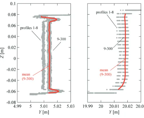
Figure 5 shows the original point clouds correspond-ing to two measurement series for target S99 at two dif-ferent positions. The nearly vertical, central parts of the point clouds correspond to the target surface, the tails and variations(∆Y) at the bottom and top correspond to parts of the trolley and of the target holder. The quantization in Z−component is due to the chosen angle increment of 0.018○
and to the fact that the measurements are taken at almost the same vertical angles in all profiles (range ap-prox. 10−5○). The standard deviation of the distances is constant over the target surface, and the target surface it-self is flat within the TLS precision.
The most striking pattern in Figure 5 is the separation of the point clouds of the first 8 profiles from those of all the remaining ones. The gap corresponds to a sudden increase of the measured distance by about 5 mm after the 8th pro-file. With less reflective targets and longer distances the measurement noise grows and eventually masks this jump when viewing the data in the point cloud domain. How-ever, we found it with equal magnitude and equal sign in all measurement series and all cycles, and also within the measurements to the control target and to the walls of the lab. The jump is due to the application of a distance cor-rection within the scanner, derived from measurements to an internal reference. This correction is determined during the first few profiles and only applied afterwards⁵. We have eliminated it from the subsequent analysis by ignoring the first few profiles of each measurement series.
The recorded signal strength values of these two mea-surement series are shown in Figure 6. The values are out-put by the scanner in units of increments (Inc) represent-ing a cardinal measure without known relation to SI units⁶. We do not see a gap like with the distances, and actually we did not find any discontinuity in the signal strength data. However, the average signal strength from profiles 9-300 is not centered within the range of values of all signal strength measurements (see bold red line, Figure 6). This suggests a drift of the signal strength values with time –
5This jump is only contained in data collected using the scanner in profile mode. When operated in 3D-mode the scanner does not store measurements obtained before determination of the internal correc-tion. Personal communication, M. Mettenleiter, Zoller+Fröhlich. 6We have not corrected these values for the impact of potential vari-ations of angle of incidence, because this impact was estimated to be significantly below the noise level.
and actually such a drift was consistently found through-out the data collection. It will be shown and discussed be-low.
We further notice that the signal-to-noise ratio of the signal strength measurements is much worse than that of the distances. Actually, the signal strength measurement noise is on the order of 3% of the measured value, con-sistent with the corresponding results reported in [9]. The average signal strength profile along the target (bold red line in Figure 6) shows a variation on the order of 1% (1σ) which is significant because this average profile is the arithmetic mean of almost 300 original profiles. So, while the Spectralon target is geometrically flat (see average pro-files in Fig. 5) it seems to have slight radiometric inhomo-geneities, as indicated by the variations of the average sig-nal strength profiles. However, the variations are within the specified radiometric flatness of the target. Similar re-sults have also been obtained with the other targets.
4.3 Representative point
The equations derived in section 4.1 refer to the distance which would be measured by the scanner at the vertical angle ˜θr, i.e., along the line MM (see Figure 2). At this
an-gle the center of the laser beam footprint hits the same sur-face patch of the target for all distances. Because of the sufficient geometric and radiometric homogeneity we can therefore analyze the data corresponding to ˜θras if they
referred to the same target surface point (representative
point) for all distances irrespective of the varying footprint
size from 3 mm at the near end to 5 mm at the far one. However, there will usually be no measurements at ex-actly the vertical angle ˜θr because of the discrete angle
increments used by the scanner and because of the jitter of the angular measurements. For the present purpose it is sufficient to pick the respective nearest neighbor in the sense of θk,i,l ≈ ˜θr from each profile within a
measure-ment series and treat the corresponding distances and sig-nal strengths as if they had been measured exactly at ˜θr.
Given the dense sampling and the negligible effect of a ver-tical deviation of less than 0.018○/2 on the measured dis-tance this is justified. We then obtain a time series of actu-ally measured distances and signal strengths of the repre-sentative point for each cycle (i.e. target), target position, and leg.
Three such time series are shown in Figure 7. They all refer to a target distance of about 5 m, and each of them contains the 300 measurements to the representative point, selected from the corresponding measurement se-ries. The jump between the first 8 profiles and the
remain-Fig. 5. Point clouds of two typical measurement series with target S99; average of profiles 9-300 is shown in bold red.
Fig. 7. Variation of distance measurements (top) and signal strength measurements (bottom) for the representative point of three differ-ent targets at a distance of 5 m.
ing ones can clearly be seen at about 0.7 seconds after the start (Figure 7, top) of the respective profile measurements, which were carried out on different days for the three tar-gets shown here. The mean value of the distances remains constant after the jump, and the standard deviation (after the jump) is 1.3 mm for the dark target S05 and only 0.3 mm for the bright one (S99), indicating high precision of all these distance measurements.
The corresponding signal strengths are shown relative to the respective first value per time series (Figure 7, bot-tom). Obviously the measured signal strength decreases by about 10% during the first 4 seconds of each profile, and slightly even afterwards. Fitting a function of type exp(−∆t/τ) as is often used to model warm-up effects, yields time constants τ between 3 and 5s. for the present data, but confirms also the visual impression that the ef-fect here decays faster in the beginning and slower later on than described by this simple model.
We see this initial decay of 10-15% with all measure-ment series and all measuremeasure-ment cycles. Since the emitted signal strength is not modified while scanning, the effect is due to warm-up of the rangefinder electronics which is only activated during data acquisition⁷, and to the chosen measurement scheme where the profile measurements are stopped during target repositioning.
7Personal communication, M. Mettenleitner, Zoller+Fröhlich.
However, we see from Figure 7 that the signal strength is almost constant within its measurement precision of 1% after 4 s, i.e., after the first 50 profiles, and that the dis-tances do not seem to be affected by this warm-up effect at all. All other measurement series which we have collected yielded similar results. So, we subsequently ignored the first 50 profiles of each series for the analysis. The results obtained further on will therefore be neither affected by the above distance jump nor by a potential bias due to the initial decay of the signal strengths.
The representative measurements Dk,i and Sk,i as
needed for the analysis according to sec. 4.1 were finally obtained by averaging the corresponding data from pro-files 51 to 300. The distances within these 250 propro-files were found to be uncorrelated and thus the standard deviation of the representative measurements is better than that of the original laser scanner measurements by a factor of 16, which helps to mitigate the impact of measurement noise on the subsequent study of systematic effects. The signal strength measurements are still slightly correlated after the 50thepoch, but also their representative measure-ments are about an order of magnitude more precise than the original measurements.
5 Analysis
5.1 Signal strengths
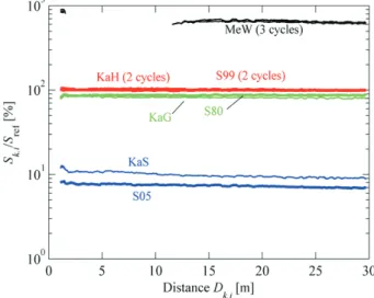
Atmospheric attenuation is negligible in the lab and at short distances. The angle of incidence is nearly constant for all data finally evaluated, and its residual variations have negligible effect on the recorded signal strengths. So, we may expect that the signal strength depends linearly on target reflectance and is inversely proportional to the sec-ond power of the target distance. This is not confirmed by our measurements (see Figure 8). For short distances (less than about 20 m), the defocusing of the laser beam causes a much slower decrease of signal strength with distance. This helps to avoid saturation of the detector with targets very close to the scanner. For distances below about 4 m, the defocussing and the shadow of certain scanner com-ponents on the detector cause even an increase of recorded signal strength with increasing distance. This behavior is qualitatively in line with the theoretical and experimental results shown in [9]. Furthermore, the scanner does not ex-port measurements any more if the signal strength exceeds a threshold of about 5×10⁶Inc. The figure shows that this is the case for the measurements to the white metal target for distances between 1.6 and 11.6 m.
Fig. 8. Signal strength from measurement cycles with different tar-gets.
With all other relevant parameters equal in this exper-iment, the signal strength at any given distance should de-pend linearly on the target surface reflectivity, and the ra-tio of the measured signal strengths should be constant over all distances. This can easily be checked using the above data. We have chosen the first leg of one of the S99 cycles as a reference and divided all measurements plotted in Figure 8 by the value of the reference at the respective distance. The result is shown in Figure 9 and confirms the constant ratios thus corroborating that the scanner emits radiation with constant power and that the signal strength measurement in increments has a stable zero value and scale.
5.2 Distance deviations
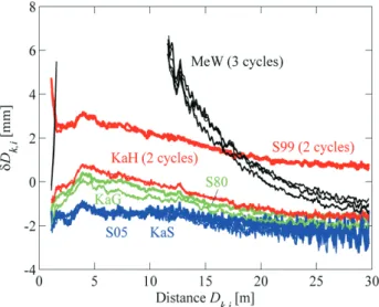
The distance deviations for the seven targets are shown as functions of the distance in Figure 10. The figure clearly shows that the distance deviations are not purely random and that there is a relation to distance.
Each target has been measured in cycles comprising at least one forward and one backward leg. So, there are at least two distance deviations for each target and each distance. Three targets were used for two cycles at differ-ent days i.e., with other targets measured in between. MeW has even been used for three independent cycles. The for-ward and backfor-ward legs, and even the multiple cycles can hardly be distinguished in Figure 10, except for one cycle of MeW which is offset by about 0.5 mm. Generally, the fig-ure indicates a very high repeatability of the test measfig-ure-
measure-Fig. 9. Ratio of recorded signal strengths to those of the first S99 cycle (Sref).
ments over a few hours (forward/backward leg) and even over longer times and with target replacement (multiple cycles). This repeatability is better than 0.1 mm for most of the data shown in Figure 10, except for the (noisier) data of the weakly reflecting surfaces S05 and KaS, and of the other targets at distances above about 20 m.
On the other hand, this means that the apparent off-sets between the various curves (again except MeW) ac-tually indicate corresponding systematic distance devia-tions of the TLS measurements. It is also clear from the fig-ure then that the distance deviations do not depend only on the target distance and would therefore not be miti-gated by TLS calibration with a model like the standard AP as introduced by [5].
Apart from the offsets and the noise level, which in-creases with distance and with decreasing surface reflec-tivity, most of the curves are similar. The patterns are simi-lar to those of the signal strengths, and locally minimum distance deviation is reached where the signal strength has a local maximum. All this suggests that there is a func-tional relation between the distance deviations and signal strength.
Cyclic deviations seem to be present at distances larger than 20 m only, and with amplitudes increasing with both increasing distance and decreasing signal strength. We need to recall that the TLS measurements were already internally corrected for effects which the manufacturer has included in the scanner software, so the data which we analyze represent only the residual deviations. Neverthe-less, the figure suggests that actually, as assumed before, the cyclic deviations are a function of distance and
sig-Fig. 10. Distance deviations determined using 7 different targets.
nal strength, not of distance alone. This is corroborated by the oscillations visible for several targets towards the right hand side of the figure (S05, KaS, KaH, and to a lesser degree also S80 and S99) with amplitudes increasing to-wards the right and with higher amplitude for the less-reflective targets. However, within the investigated dis-tance range the visually recognizable cyclic deviations are small compared to other systematic deviations and are thus not further investigated herein.
The highly reflective target MeW is apparently prob-lematic in this investigation in several respects. First, one of the three repeated cycles stands apart. Using a subse-quent experiment, we found out that this is most likely because target orthogonality with respect to the interfer-ometer beam II (see sec. 3.1) and thus also with respect to the measurement beam of the scanner had not been reproduced with sufficient accuracy during this particu-lar cycle. We found that changes of less than 0.1○of the angle of incidence could already produce signal strength changes on the order of 20% and mm-level changes of distance deviation for this particular target. Secondly, the other curves suggest that higher surface reflectivity causes greater distance deviations (i.e., apparently longer dis-tances); MeW is about six times more reflective than S99 but still yields smaller distance deviations at distances be-yond 20 m. Also, the significant offset between KaH and S99 which have approximately the same surface reflectiv-ity indicates that there is not only a dependence of δD on signal strength but there may be significant surface pene-tration or other effects as well.
Plotting the deviations versus signal strength rather than distance (Figure 11) clarifies (i) that the deviations
Fig. 11. Measured distance deviations shown in relation to the corre-sponding measured signal strengths.
are also not only a function of signal strength, but (ii) that there is nevertheless a clear relation to signal strength. MeW seems to stand out less in this display than in the previous one; it merely occupies mostly a range of signal strengths which are not present in the data of the other targets. Instead, it is clearer from this figure than from Fig-ure 10 that there are also some outliers within the S99 data at short distances.
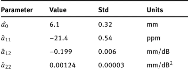
In order to check whether the distance deviations can possibly be modelled as a function fcof measured
quanti-ties, we have selected the following bivariate polynomial ansatz: fc(D, S) ∶= a0+ a11⋅ D + a12⋅ SdB + a21⋅ D2+ a22⋅ S2 dB + a23⋅ D ⋅ SdB (11) with SdB ∶= 20 ⋅ log10S. (12) We have chosen the logarithmic scale (SdB in dB) for the
signal strength because a comparison of Figure 11 with a corresponding figure showing S in linear scale indicated that the former was more linearly related to δD. We then estimated the unknown coefficients a0, . . . , a23using or-dinary least-squares parameter estimation from the given data δDk.i, Dk,iand Sk,i. However, we only used the data
from one cycle of KaH and one cycle of KaS, as these tar-gets represent very low and very high reflectivity and most other targets are in between. Using a significance test of the estimated parameters and repeated estimation with sub-sets of the parameters, we found that four of the parame-ters in this model are sufficient to describe a major part of
Table 3. Estimated parameters of model (13) and their associated standard deviations (Std).
Parameter Value Std Units
ˆ a0 6.1 0.32 mm ˆ a11 −21.4 0.54 ppm ˆ a12 −0.199 0.006 mm/dB ˆ a22 0.00124 0.00003 mm/dB2
the deviations found within this experiment: ˆfc(D, S) ∶= ˆa0+ ˆa11D+ ˆa12SdB+ ˆa22S
2
dB. (13)
The numeric values resulting from the estimation are given in Table 3. The bias term ˆa0may contain a contribution from an actual distance bias, but it also absorbs the small deviation of the assumed constant term C0from the un-known true term ˜C0(see sec. 4.1) and is therefore just a nui-sance parameter here. The other terms indicate that there is a (small) scale deviation and they corroborate the hy-pothesis that there is a dependence of distance deviations on both signal strength and distance which can be mod-elled.
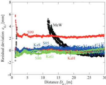
The residual deviations
ek,i= δDk,i− ˆfc(Dk,i, Sk,i) (14)
after application of this estimated model are shown for all data in Figure 12. A comparison of this figure with Figure 10 suggests that in fact the simple model of eq. (13) can al-ready explain a major part of the distance variations (see Table 4) despite the fact that it was only estimated from a subset of the data of two targets. However, it also clearly shows that targets S99 and MeW are not well represented by this model. The reasons are different. Pure Spectralon achieves its highly Lambertian behavior by multiple re-flections within the first few tenths of a millimeter of its surface and subsurface. So, very likely there is significant surface penetration⁸ with target S99 while there is very lit-tle or no surface penetration with the other targets. Such an effect cannot be modelled by equations which only use distance and signal strength measurements. Target MeW with its strong directional reflection causes effects that are different from the ones encountered with diffusely reflect-ing targets. We may expect that targets with surface reflec-tivity significantly higher than 100% can also not be ac-commodated using the same function as for targets with
8 The resulting distance bias will be typically greater than the actual penetration depth because of the reduced wave propagation speed within the target medium.
Table 4. Standard deviation (Std)† of distance deviations before and after application of the model estimated only from KaH (1stcycle)
and KaS.
Targets Std of δD Std of e Improvement
in mm in mm by the model
KaH (1stcycle) & KaS 0.87 0.18 79%
All except S99 & MeW 0.79 0.28 65% † The Std is used here instead of an rms because of the arbitrary offset affecting all δD.
Table 5. Correlations of estimated parameters of model (13).
Parameter ˆa0 ˆa11 ˆa12 a22ˆ
ˆ a0 1 ˆ a11 −0.114 1 ˆ a12 −0.997 0.058 1 ˆ a22 0.991 −0.028 −0.998 1
mostly diffuse reflection. However, strong directional re-flection could easily be detected by comparing the mea-sured signal strength to a distance dependent threshold representing a reflectivity of e.g., 100%.
The fit can of course be still improved by including the data of all targets except MeW into the parameter estima-tion process, and estimating target specific offsets (e.g., to be interpreted as effect of differential surface penetration). However, we leave this to a more focused later study be-cause the estimated parameters are highly correlated with the present data (see Table 5), indicating that they can-not be separated (and therefore they should can-not be inter-preted individually). It may be necessary to have data over a longer distance range and additional data identifying the offset to better separate the parameters of the model.
An extended range of the experiment would also al-low investigating whether there are longer periodic cyclic deviations. Such deviations would mostly be absorbed by the estimated scale factor in the above investigation. How-ever, it will be very challenging to find a suitable environ-ment and setup providing sufficiently accurate distances for comparison to the laser scanner data beyond 30-50 m. This is left for a future investigation therefore.
Fig. 12. Residual distance deviations after application of the model (13).
6 Conclusions
Using a carefully planned and executed experiment we have investigated whether variations in surface reflectiv-ities cause systematic deviations of phase-based RL-EDM. We indeed found that such variations may cause apparent distance variations of a few mm with diffusely reflecting target surfaces and more with directionally reflecting ones. While such distance deviations may seem small, they are of the same order of magnitude other parameters usu-ally included in the AP model for laser scanner calibration may reach. Neglecting these (additional) deviations may adversely affect RL-EDM measurements or TLS measure-ments if the data processing allows reduction of noise e.g., by fitting geometric primitives to the data or by averaging over a time series of data. Furthermore, the surface reflec-tivity may change without the geometry of an object chang-ing. In this case, apparent deformation or motion may be detected which is in reality an artefact caused by changed reflectivity and thus by changed signal strengths at the de-tector.
In view of monitoring using TLS, in view of high-precision surface reconstruction, and in view of laser scan-ner self-calibration the dependence of distance devia-tions on signal strength or equivalently surface reflectivity should be taken into account. We have shown that a bivari-ate quadratic polynomial in distance and signal strength can already explain the variations that we found over dis-tances up to 30 m with a particular scanner. There may be a chance to actually model the deviations for a broader range of distances and instruments.
However, further investigations are required to ana-lyze the effects for distances typically encountered with monitoring and high precision surveying, i.e., a few hun-dred meters, and to better understand whether it is useful and possible to distinguish between mainly diffuse reflec-tion and significant or mainly directed one in terms of devi-ations models and mitigation. These investigdevi-ations should also include the impact of different beam characteristics, footprint and raw-data evaluation schemes in order to gen-eralize the findings to instruments which may differ in this respect, e.g., total stations. Finally, they should be ex-tended to modelling the distance noise as a function of sig-nal strength. The present investigation may serve as a start-ing point.
Acknowledgement: The authors are indebted to Mr. Presl
(TU Graz) for help with the setup and laboratory work, to Mr. Mettenleiter (Zoller+Fröhlich) for information and clarifications regarding the scanner, and to Prof. N. Pfeifer (TU Vienna) for discussion and comments on a draft of this paper.
References
[1] Böhler W., Bordas Vicent M., Marbs A., Investigating Laser Scanner Accuracy, Proceedings of the XIXth CIPA International
Symposium, Antalya, Turkey, 2003, 696–702.
[2] Dorninger P., Nothegger C., Pfeifer N., Molnár G., On-the-job detection and correction of systematic cyclic distance mea-surement errors of terrestrial laser scanners, Journal of Applied
Geodesy2 (2008), 191–204.
[3] Ge X., Wieser A., Wunderlich Th., Calibration and analysis of a terrestrial laser scanner, ISPRS Journal of Photogrammetry and
Remote Sensing97 (2015), (in preparation).
[4] Joeckel R., Stober M., Huep W., Elektronische Entfernungs- und
Richtungsmessung und ihre Integration in aktuelle Position-ierungsverfahren, Heidelberg, Herbert Wichmann Verlag, 2008
(German).
[5] Lichti D., Error modelling, calibration and analysis of an AM-CW terrestrial laser scanner system, ISPRS Journal of
Photogram-metry & Remote Sensing61 (2007), 307–324.
[6] Linstaedt M., Kersten Th., Mechelke K., Graeger T., Sternberg H., Phasen im Vergleich – erste Untersuchungsergebnisse der Phasenvergleichsverfahren, Photogrammetrie - Laserscanning
- Optische 3D-Messtechnik, Beiträge der Oldenburger 3D-Tage
2009, Luhmann Th., Müller C., Oldenburg, Verlag Herbert Wich-mann, Heildelberg, 2009, 53–64 (German).
[7] Molnár G., Pfeifer N., Ressl C., Dorninger P., Nothegger C., On-the-job Range Calibration of Terrestrial Laser Scanners with Piecewise Linear Function, Photogrammetrie, Fernerkundung, Geoinformation 1, 2009, 9–22.
[8] Palmer J. M., Grant B. G., The Art of Radiometry, Washington, SPIE Publications, 2009, p62.
[9] Pfeifer N., Höfle B., Briese Ch., Rutzinger M., Haring A., Anal-ysis of the backscattered energy in terrestrial laser scanning data, The International Archives of the Photogrammetry, Remote
Sensing and Spatial Information SciencesVol. XXXVII. Part B5.
Beijing 2008, 1045–1052.
[10] Reshetyuk Y., A unified approach to self-calibration of terres-trial laser scanners, ISPRS Journal of Photogrammetry & Remote
Sensing65 (2010), 445–456.
[11] Rüeger J. M., Electronic Distance Measurement, An
Introduc-tion, Berlin Heidelberg New York, Springer, 1996.
[12] Schulz T., Calibration of a Terrestrial Laser Scanner for Engi-neering Geodesy, PhD thesis, ETH Zürich, 2007, No. 17036.
[13] Vennegeerts H., Richter E., Paffenholz J.-A., Kutterer H., Hennes M., Genauigkeitsuntersuchungen zum kinematischen Einsatz terrestrischer Laserscanner. AVN(4), 2010, 140–147 (German).
[14] Zámečníková M., Kutterer H., Suhre H., Vennegeerts H., Unter-suchung des Distanzmesssystems Imager 5006. Photogramme-trie - Laserscanning - Optische 3D-Messtechnik, Beiträge der Oldenburger 3D-Tage 2009, Luhmann Th., Müller C., Heildel-berg, Verlag Herbert Wichmann, 2009, 45–52 (German).