PrePeP – A Tool for the Identification and Characterization of Pan Assay Interference Compounds

HAL Id: hal-01939468

https://hal.archives-ouvertes.fr/hal-01939468

Submitted on 12 Dec 2018

HAL is a multi-disciplinary open access

archive for the deposit and dissemination of

sci-entific research documents, whether they are

pub-lished or not. The documents may come from

teaching and research institutions in France or

abroad, or from public or private research centers.

L’archive ouverte pluridisciplinaire HAL, est

destinée au dépôt et à la diffusion de documents

scientifiques de niveau recherche, publiés ou non,

émanant des établissements d’enseignement et de

recherche français ou étrangers, des laboratoires

publics ou privés.

PrePeP – A Tool for the Identification and

Characterization of Pan Assay Interference Compounds

Maksim Koptelov, Albrecht Zimmermann, Pascal Bonnet, Ronan Bureau,

Bruno Crémilleux

To cite this version:

Maksim Koptelov, Albrecht Zimmermann, Pascal Bonnet, Ronan Bureau, Bruno Crémilleux. PrePeP

– A Tool for the Identification and Characterization of Pan Assay Interference Compounds. 24th

ACM SIGKDD International Conference on Knowledge Discovery & Data Mining, Aug 2018, Londres,

United Kingdom. pp.462-471, �10.1145/3219819.3219849�. �hal-01939468�

PrePeP – A Tool for the Identification and Characterization of

Pan Assay Interference Compounds

Maksim Koptelov

Normandie Univ, UNICAEN, ENSICAEN, CNRS - UMR GREYC

Caen, France [email protected]

Albrecht Zimmermann

Normandie Univ, UNICAEN, ENSICAEN, CNRS - UMR GREYC

Caen, France [email protected]

Pascal Bonnet

Ronan Bureau

Bruno Crémilleux

Normandie Univ, UNICAEN, ENSICAEN, CNRS - UMR GREYC

Caen, France [email protected]

ABSTRACT

Pan Assays Interference Compounds (PAINS) are a significant prob-lem in modern drug discovery: compounds showing non-target specific activity in high-throughput screening can mislead medici-nal chemists during hit identification, wasting time and resources. Recent work has shown that existing structural alerts are not up to the task of identifying PAINS. To address this short-coming, we are in the process of developing a tool, PrePeP, that predicts PAINS, and allows experts to visually explore the reasons for the predic-tion. In the paper, we discuss the different aspects that are involved in developing a functional tool: systematically deriving structural descriptors, addressing the extreme imbalance of the data, offering visual information that pharmacological chemists are familiar with. We evaluate the quality of the approach using benchmark data sets from the literature and show that we correct several short-comings of existing PAINS alerts that have recently been pointed out.

KEYWORDS

Discriminative graph mining, chemoinformatics, structure activity relationships

ACM Reference Format:

Maksim Koptelov, Albrecht Zimmermann, Pascal Bonnet, Ronan Bureau, and Bruno Crémilleux. 2018. PrePeP – A Tool for the Identification and Characterization of Pan Assay Interference Compounds. In KDD ’18: The 24th ACM SIGKDD International Conference on Knowledge Discovery & Data Mining, August 19–23, 2018, London, United Kingdom. ACM, New York, NY, USA, 10 pages. https://doi.org/10.1145/3219819.3219849

1

INTRODUCTION/MOTIVATION

Modern drug development follows what is arguably a four-step progress: 1) high-throughput screening (HTS) to find compounds showing activity regarding a therapeutic target or its surrogates (so-called “hits”), 2) more fine-grained evaluation and limited opti-mization to identify promising “leads”, 3) additional optiopti-mization and pre-clinical testing, 4) clinical testing.

KDD ’18, August 19–23, 2018, London, United Kingdom 2018. ACM ISBN 978-1-4503-5552-0/18/08. . . $15.00 https://doi.org/10.1145/3219819.3219849

Depending on the test readout used during the first step, certain molecules can emerge as hits that do not actually interact with the target, e.g. reduction in harmful cells in a cell culture can be achieved by peroxide production. Such false positives are impossi-ble to optimize for the therapeutic target and therefore do not lead to successful drug development, wasting time and resources. A par-ticularity of non-specific interaction is that such compounds seem to show activity in different, potentially independent biochemical assays, hence their name “frequent hitters” (FHs). Filtering out FHs at an early step is clearly desirable to avoid leading drug developers down dead ends. The problem has been identified in the literature by Baell et al. [6], where those compounds have been dubbed “Pan-Assay INterference compoundS” (PAINS), and subsequent studies have shown their repeated presence in publications introducing supposed leads [33, 36]. A recent joint editorial of the editors-in-chief of journals of the American Chemical Society [4] has drawn special attention to this problem.

Baell et al. also introduced a number of structural alerts, based on their analysis of a proprietary compound database, which have since found ample use in PAINS detection. Yet as shown in [17] and [26], those alerts suffer from low recall – missing many FHs – while at the same time sweeping up many “infrequent hitters” (iFHs). Capuzzi et al. [17] indicate that one possible issue with existing PAINS alerts is that they are based on very few FHs, in some cases as few as a single one. An alternative method to identify PAINS is therefore clearly needed.

Pattern mining techniques, taking inspiration from statistics, have always allowed to constrain the minimum empirical support or effect size [44]. Using quality measures that contrast two classes against each other, e.g. growth rate [29, 31] or statistical measures [15, 46], allows to mine substructures that are representative of FHs or iFHs.

We propose to use such techniques to derive new structural alerts, which we combine with machine learning models to predict PAINS. To develop the approach, we had to address three issues: 1) the extreme imbalance of the underlying data, which by nature contains very few FH examples, 2) how to derive a small set of meaningful structural descriptors, and 3) how to create an accurate predictive model that is at the same time interpretable, to facilitate acceptance by researchers in medicinal chemistry and aid further

scientific research in the field. We have validated our goals and design choices with our partners and co-authors from ICOA and CERMN, two medicinal chemistry laboratories in Orléans and Caen, respectively, and evaluated the approach on recent benchmark data sets from the literature.

PrePeP, of which we describe the prototype in this paper, con-tains three ingredients: 1) representative subgraphs mined off-line, 2) decision tree classifiers that have also been learned off-line, and 3) a graphical interface that allows to explore the predictions for unseen molecules as well as which subgraphs were involved in the prediction.

The rest of the paper is structured as follows: in the following section we provide definitions and notation. We touch on related work in Section 3 and we discuss data preparation in Section 4. In Section 5, we explain how the structural descriptors have been derived and the model built, which we evaluate in Section 6. In Section 7, we describe the tool we have developed before concluding in Section 8 and providing perspectives.

2

DEFINITIONS

We begin by formally defining the concepts that we have informally introduced in the introduction.

Definition 2.1. Letℳ a set of molecules, with each m ∈ ℳ of the form (x, y), x being the representation of the molecule and y ∈ {0, 1}dits activity profile.

Note, that we do not concretely specify the molecule representa-tion – different oprepresenta-tions will be discussed in Secrepresenta-tion 4. The activity profile results from the (post-processed) outcomes of different HTS assays, withd the number of bioassays in which a compound has been tested.

Definition 2.2. A frequent hitter (FH) is a molecule (x, y) ∈ ℳ : ||y|| ≥ θ, with θ a user-specified threshold. In addition, we call molecules (x, y) ∈ ℳ : ||y|| < θ infrequent hitters (iFH), and (x, y) ∈ ℳ : ||y|| = 1 one-hitters (1H).

The user-defined thresholdθ specifies how often a compound needs to show activity to be considered FH. When appropriate, we will refer to the subsets made up of FHs/iFHs/1Hs asℳF H, ℳiF H,ℳ1H, respectively. Later on, we will speak – somewhat informally – of Dark Chemical Matter (DCM), molecules for which ||y|| = 0,d >> 10, i.e. compounds that have been assayed (very) often.

In this work, we consider molecules as graphs, i.e. representing them in terms of their 2D structure.

Definition 2.3. A graph is a tuple ⟨V , E, λv, λe⟩, withV a set of vertices,E ⊆ V ×V a set of edges, λv:V 7→ 𝒜va labeling function mapping vertices to elements of an alphabet of possible vertex labels, andλe:E 7→ 𝒜ea labeling function for edges.

Any given molecule can be represented as a graph of which the vertices are labeled with atom names, and edges with atomic bonds.

Definition 2.4. Given two graphsG = ⟨V , E, λv, λe⟩, G′ _{= ⟨V}′_{, E}′_{, λ}

v′, λ_e′⟩,G′is a subgraph ofG iff V′ ⊆V ∧ E′ ⊆

E ∧ ∀v ∈ V′_:λ

v′(v) = λ_v(v) ∧ ∀e ∈ E′:λ_e′(e) = λ_e(e). We also

say thatG′matchesG (G′⪯G). Given a set of graphs 𝒢 , we also

define the cover ofG′:cov(G′, 𝒢 ) = {G ∈ 𝒢 | G′ ⪯G} and its support:supp(G′, 𝒢 ) = |cov(G′, 𝒢 )|.

In addition, we require of our subgraphs that they be connected. Definition 2.5. A graphG = ⟨V , E, λv, λe⟩ is connected iff∀u,v ∈ V : ∃v1, . . . ,vn :v1= u ∧ vn= v ∧ (vi,vi+1) ∈E.

3

RELATED WORK

3.1

PAINS identification/characterization

The terms PAINS has been coined in [6], the authors of which proposed a set of structural alerts to identify and exclude PAINS. Following work has mainly focused on identifying PAINS mistak-enly published in the literature and identifying their mechanisms [7, 8, 20, 33, 36, 40, 41].

Criticism of Baell et al.’s filters is more muted, with one notable publication [30] arriving at conclusions contrary to those of [41]. Recently, two publications [17, 26] have called the usefulness of existing structural alerts into question. Capuzzi et al. show existing alerts miss a large proportion of FHs in an independently curated molecular data set, yet match a large proportion of iFHs, success-fully marketed drugs (arguably a subset of 1Hs), and even DCM compounds. In trying to understand this behaviour, they illustrate that many (190 of 480) of the original alerts have been derived from a single compound each.

Alternatives are, to the best of our knowledge, rare so far, with the exception of [45], which proposes tagging compounds with different scaffolds, each of which has a Bayesian-inspired FH score.

3.2

(Q)SAR modeling

(Quantitative) structure activity relationship modeling is concerned with using statistical or machine learning models to predict a com-pounds’ activity w.r.t. a given target, based on its structural proper-ties. Work in this field is well-established [39] and on-going [19, 42]. Several authors [23, 27] have drawn attention to the importance of the interpretability of derived models – black box classifiers do not help in isolating and optimizing effective components – and to the unavoidable trade-off with accuracy that will result from it. (Q)SAR methods typically assume a previously defined therapeutic target for which bioassay data exists.

3.3

Pattern mining

Transactional graph mining has often been motivated with (fre-quent) substructure discovery in molecular data. The probably best-known algorithm is gSpan [44] but there exist alternatives [25, 28, 35], and experimental studies [34, 43] have shown incon-clusive results regarding their relative merits. By using the result presented in [32], which exploits the convexity of certain quality measures, such approaches can be used to find discriminative sub-structures for the (Q)SAR problem [15, 46]. Alternatively, one can use the classic frequent pattern mining approach and combine the results to arrive at discriminative conjunctions of patterns [29, 31].

4

DATA PREPARATION

The data we base our model on have been curated by Capuzzi et al. for their publication [17]. As usual in that community, the data are publicly available in the form of PubChem IDs and SMILES

PrePeP – Identification and Characterization of PAINS KDD ’18, August 19–23, 2018, London, United Kingdom

strings [24] at http://pubs.acs.org/doi/abs/10.1021/acs.jcim.6b00465. Following Baell et al. [6], each compound in the data set has been evaluated in six assays, and the activity threshold for declaring a compound FH has been set toθ = 2.

Molecules were standardised using the tool VSPrpep [22], giving rise to a graph representation. Starting from that representation, each chemical compound was described using the RDKit Morgan fingerprint implemented in Knime [9] with a radius of three chem-ical bonds [3] as used in a previous study [12]. The fingerprint composed of 0 and 1 bits takes into account the neighborhood of each atom by exploring the adjacent atoms in a three connected bounds. Numerical molecular 0D-descriptors were derived using Pipeline Pilot [10], giving rise to 192 numerical descriptors. In other words, each compound is available in the form of a graph, a bitstring of fingerprints, and a set of numerical descriptors.

Additional data that we use in Section 6 for evaluation is available in graph form. All data can be downloaded at https://zimmermanna. users.greyc.fr/supplementary-material.html.

5

SUBSTRUCTURE MINING AND MODEL

LEARNING

As shown in Section 4, the options for representing molecules are plentiful. So plentiful, in fact, that the sheer number of chemical fin-gerprints – 107k – threatens to introduce a curse-of-dimensionality issue, as well as significantly slow down any learner used to induce a model. In addition, the available data is highly imbalanced, a prob-lem that needs to be addressed to enable feature construction and model learning. The model itself, finally, should be interpretable, both to convince experts to accept the predictions and to facilitate further scientific progress on the application side. In this section, we discuss how we addressed those three challenges.

5.1

Discriminative subgraph mining

Chemical fingerprints are derived from chemical background knowl-edge and usually based on a very low minimum support in the data, hence their large number. Quality measures that score how well subgraphs discriminate between two classes, on the other hand, can capture much more information in a smaller set of patterns. We therefore chose to use gSpan, augmented with the capability to use the information gain measure via upper-bound pruning, to mine discriminative subgraphs.

Definition 5.1. Let the data setℳ consist of two subsets ℳF H, ℳiF H :ℳF H∩ℳ_{iF H} = ∅ ∧ ℳ_{F H}∪ℳ_{iF H} = ℳ . The entropy of the data set is:

H(ℳ ) = −|ℳ_{|ℳ |}F H| · log₂ |ℳF H| |ℳ | − |ℳ_{iF H}| |ℳ | · log2 |ℳ_{iF H}| |ℳ | , and the information gain of a subgraphG w.r.t. ℳ :

IG(G, ℳ ) = H(ℳ ) −supp(G,ℳ )_{|ℳ |} ·H(cov(G, ℳ )) −|ℳ |−supp(G,ℳ )_|

ℳ | ·H(ℳ \ cov(G, ℳ ))

Information gain rewards subgraphs that change the distribution in the covered and uncovered subsets towards one of the two classes. Our hypothesis is that there are shared structural characteristics of FHs that can be quantified via information gain, whereas iFHs are too heterogeneous for shared patterns to appear. There are other

convex quality measures that could be chosen but there are no well-founded selection criteria, apart from the fact that normalized measures, like information gain, are preferable to unnormalized ones, such asχ2, which overly reward patterns with very small effects if the effect size is large.

The decision for gSpan is mainly a practical one: with an imple-mentation for discriminative pattern mining provided by Siegfried Nijssen, there was no need to implement a miner ourselves. The de-cision to mine graphs instead of sequences, which work as well and are easier to mine [15], was deliberate, however: when presenting results to domain experts, graph patterns, particularly those includ-ing cycles, are more informative. We represented all molecules in the form of hydrogen-suppressed graphs, i.e. all vertices labeled with “H” were removed from the graphs. We have mined the top-100 subgraphs according to information gain.

5.2

Balancing the data

The data set described in Section 4 has size |ℳ | = 153539, of which only a very small subset are FHs: |ℳF H|= 902 when using the thresholdθ = 2 (meaning that molecules are active on at least two assays). Such an imbalance will have a negative impact both on subgraph mining, and on model learning. On subgraph mining because subgraphs that split off a certain amount of iFHs while present in a majority of iFHs and all FHs would receive elevated information gain scores without being representative of FHs. On model learning because a model that always predicts the majority class, i.e. iFHs, will achieve an accuracy of 99.41%.

The recommended solution for such a setting is to undersample the majority class to create a balanced data set. In our case, creating a single undersample would remove the overwhelming majority of iFHs, without any guidance regarding which instances to keep. We elected therefore to perform repeated sampling, using all FHs every time and randomly sampling an equal amount of iFHs from the data. To ensure that we use every iFH at least once, we need at least 171 samples but since we would like to contrast different combinations of iFHs against the FHs in the data, we scaled up to 200 samples.

5.3

The predictive model

The task that the predictive model is supposed to address is a form of SAR – instead of having a single therapeutic target, the target class is that of frequent hitters, i.e. molecules that show activity regarding different targets. The general setting remains the same, however: given molecules described in terms of their structure and labeled by an activity indicator, find a model that reliably predicts the latter based on the former.

As indicated in Section 3, an important aspect of SAR models is interpretability. Experts are more likely to accept predictions when they are presented with explanations for those predictions in a language they understand, an issue not limited to the SAR setting [37], and SAR models are, after all, only a means to an end, that end being an understanding of biochemical mechanisms and further scientific progress in the domain.

The interpretability constraint rules out powerful non-symbolic learners such as support vector machines [18], or neural networks, particularly those used in deep learning approaches [38]. Decision

tree learners are prime representatives of interpretable models, even if using them would theoretically trade-off accuracy against interpretability. Practically, on the other hand, combining decision trees into an ensemble using Bagging [13] has been shown to lead to very good results. The resampling described in the preceding section is similar to Bagging – not identical, because the instances of one class remain fixed – so we would expect good performance of an ensemble of decision tree classifiers as well.

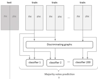
The full workflow is therefore as follows: 1) we create 200 data sets with equal amounts of FHs and iFHs by sampling fromℳF H, 2) we mine the top-100 discriminative subgraphs from each data set, 3) we encode each molecule with the numerical descriptors described in Section 4 and a hundred-dimensional bit-vector indicating the presence/absence of the subgraphs mined from this data set, 4) we learn one decision tree classifier (DT) for each data set. An unseen molecule is encoded in terms of its numerical descriptors and the discriminative subgraphs for each of the 200 training sets and clas-sified by the respective decision trees. The final classification is derived as a majority vote of all 200 DTs’ predictions, in case of a tie the majority class (iFH) is predicted. A schema of the process is shown in Figure 1.

Figure 1: Schema of the model construction workflow.

6

EXPERIMENTAL EVALUATION

In this experimental evaluation, we evaluate the quality of the model described in the preceding section. Concretely, the first question is which representation reveals itself to be most beneficial for the prediction task, and whether decision tree classifiers can, as we have reasoned above, deliver acceptable quality for FH prediction in a well-curated data set. We then evaluate whether the model’s performance transfers to other compounds, and compare to the PAINS alerts criticized by Capuzzi et al..

6.1

Experimental setup

In total, we have used three data sets, all proposed by Capuzzi et al. in [17]:

(1) The data set described in the preceding sections, comprised of 902 FHs and 152,637 iFHs. We use these data for the proof-of-concept experiment that evaluates whether a model accu-rately predicting FHs and iFHs can be learned.

(2) A data set of 73,333 compounds that have each been eval-uated in at least 25 separate bioassays, randomly sampled from the PubChem database [2]. The data set is separated into those compounds containing PAINS alerts as originally defined in [6], hereafter referred to as Random-PAINS (14,611 compounds), and those not containing PAINS alerts (Random-NoPAINS, 58,722 compounds). These data serve two purposes: on the one hand they allow us to evaluate whether our model presents a clear alternative to the PAINS alerts proposed in [6]. On the other hand, we will assess whether a model de-rived from a particular bioassay transfers to other settings. (3) A data set of 3570 DCM compounds (tested in at least 100 bioassays) that contain PAINS alerts. Those data should ide-ally never be classified as active, let alone FH, something that existing PAINS alerts fail to do, and that we expect our model to be able to do.

As mentioned above, we used Siegfried Nijssen’s gSpan im-plementation for discriminative subgraph mining for the graph mining step. Data sampling was implemented in Python 2.7, us-ing the networkx library [5] (version 1.11) for subgraph match-ing, and scikit-learn’s [16] (version 0.17.1) decision tree learner, an implementation of CART [14]. After internal validation, mini-mum leaf size for decision trees was fixed to 3% of training data. The code for our experiments can also be downloaded at https: //zimmermanna.users.greyc.fr/supplementary-material.html.

6.2

Performance evaluation for FH

classification

To assess the model’s performance, we performed three different ten-fold cross-validations on the data set comprised of FHs and iFHs:ℳF Hwas separated into 10 folds, and for each fold a corre-sponding number of iFHs sampled. We evaluated three settings for the test fold: 1) balanced data, 90/91 FHs : 90/91 iFHs, 2) slight imbalance, 90/91 FHs : 900/910 iFHs, 3) severe imbalance, 90/91 FHs : 9000/9100 iFHs. The first setting is the ideal case in which the distribution of classes in the test data is the same as in training data, whereas the third setting is much closer to a real-life setting in which iFHs will significantly outnumber FHs. For training folds, we sample 200 times 812/811 iFHs from those not contained in the test fold. As a side-effect, this means that different training samples for the imbalanced test settings will be much more redundant, and that the “independently and identically distributed” (i.i.d.) assumption underlying inductive learning is violated for the test data.

We report several performance measures:

• Accuracy: the ratio of true positives (TP) – compounds cor-rectly classified as FH – and true negatives (TN) – compounds correctly classified as iFHs – over all predictions:

PrePeP – Identification and Characterization of PAINS KDD ’18, August 19–23, 2018, London, United Kingdom

• Precision: the ratio of TP over all compounds classified as FH:

prec =_{T P + FP}T P

Precision measures whether a model is specific enough to mainly classify instances of the positive class (FH) as positive. This gives additional insight into the accuracy score. • Recall: the ratio of TP over all FHs in the test data:

rec =_{T P + FN}T P

A model that classifies very few instances as FH, e.g. by clas-sifying almost all instances as iFHs, can achieve very good accuracy and precision, especially on imbalanced data, while failing at its final task: filtering out frequent hitters. Recall measures whether a model is general enough to classify a large proportion of the positive class as positive.

• Area under receiver operating curve (AUC): evaluates whether true positives are usually ranked above or below false posi-tives when sorting predictions by confidence.

6.2.1 ClassifyingℳF HvsℳiF H. Table 1 shows the results for three different representations: only discriminative subgraphs, only numerical descriptors, combination of both. For each performance measure, we report the average value over all ten folds and the stan-dard deviation. In the case of the balanced data, all three feature sets show good performance, with numerical descriptors improving the performance of subgraphs. Precision and recall are high, indi-cating that FHs are correctly classified and recovered. This changes as soon as we pass to the imbalanced data sets: while using only subgraphs gives similar results as before, including numerical de-scriptors deteriorates performance. Not only are accuracies lower than for subgraphs but precision drops precipitously while recall stays high, which means that while those models do classify many FHs as such, they also sweep up many iFHs and classify them incor-rectly. Using only subgraphs does better at classifying iFHs as iFH but loses some coverage on the FHs in the process. Results for the latter also become more unstable while average accuracy increases compared to the balanced setting, indicating that for certain test folds the more redundant training data is not representative enough. Yet a severe deterioration as a result of the violation of the i.i.d. assumption cannot be observed.

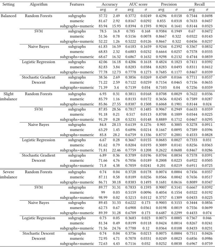
6.2.2 Test of different classifiers. We did not only test decision trees, though. Table 4 in the Appendix section shows evaluation results for a number of different classifiers trained in the same manner as the decision trees, and used in a majority vote. As can be seen from comparison with Table 1, other techniques seem to better exploit numerical features. Looking more carefully at precision and recall results, however, shows that other classifiers do not manage to improve on the low precision or recall values decision trees suffer for imbalanced data. Furthermore, decision trees perform consistently better when using only subgraphs and are, after all, more easily interpretable.

6.2.3 ClassifyingℳF H vsℳ1H. As an additional evaluation, we removed all compounds not showing activity at all and only mined on the subset containing FHs and 1Hs. This data set is sig-nificantly smaller, |ℳ1H|= 2358, |ℳ_{F H}| = 902, and much less

imbalanced than the full data (27.67% : 72.33%). We therefore do not subsample but mine subgraphs and learn decision trees directly, in the context of a stratified ten-fold cross-validation, i.e. enforcing the same class distribution in test as in training data.

As Table 2 shows, the trends of the imbalanced test data can also be found here: using only subgraphs gives better accuracy and much better precision. At the same time, recall is clearly lower than in the preceding experiments but this is an acceptable outcome: while we want to filter out FHs, we want to avoid doing this at the expense of 1Hs, which might be viable drug leads. The final realization is that contrasting FHs and 1Hs apparently gives rise to less discriminative subgraphs. This is an expected results since we would assume that the differences between compounds showing different levels of activity are less pronounced than between those showing activity and no activity at all. Based on those results, we use only discriminative subgraphs as compound representation going forward, and the entire data set of FHs and iFHs as mining/training base.

6.3

Model evaluation on randomly sampled

compounds

To evaluate the performance of our model on the Random-PAINS/ Random-NoPAINS data set, we used the full FH/iFH data set for subgraph mining and model building. The resulting subgraphs were used to encode the test data and majority vote classification performed, as described in Section 5.

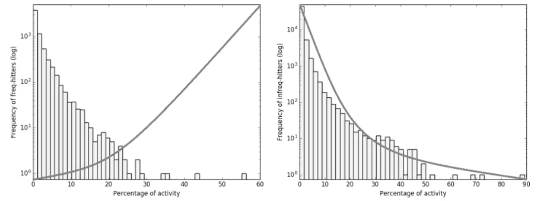
Rows two through five of Table 3 show the predictions of our model on the Random-PAINS and Random-NoPAINS subsets, re-spectively. The results show that the PAINS alerts proposed by Baell et al. and our model are very much not in agreement, i.e. we offer a clear alternative to existing filters. An additional question is, however, if our model does indeed separate frequent hitters from infrequent hitters. To this end, for the Random-PAINS classified as FH, we plot a histogram for different percentages of activity over all assays they have been tested in (Figure 2, left-hand side). The same plot can be seen for Random-PAINS classified as iFH on the right-hand side of Figure 2, and for Random-NoPAINS in Figure 3. Ideally, we would like compounds classified as iFH to be clustered on the left of the plots, showing low activity, and FHs to be clustered on the right. To illustrate this, we have also plotted lines in both figures, showing this ideal behavior. As we can see, our model does not yet achieve this ideal behavior. There are several possible explanations: first, the data set used for subgraph mining learning comes from a particular type of bioassay, AlphaScreen [21]. As explained in the introduction, different assays use different readout methods and offer therefore different conditions for PAINS to occur. Second, we have used a hard threshold to define FHs but a relative threshold, i.e. percentage of activity, might be more appropriate. Third, some compounds do act on several different targets and are of great interest in polypharmacology. Those three issues are inherent in the application setting we address here: since the mechanisms for the occurrence of PAINS are not yet clear, we cannot neatly resolve or rule out any of those effects. We intend to continue working in this direction, however.

Table 1: Evaluation of the performance of the majority vote decision tree model for different feature sets and different ratios of FHs and iFHs in the test data

Setting Features Accuracy AUC score Precision Recall avg σ avg σ avg σ avg σ Balanced subgraphs 80.00 16.67 0.80 0.17 0.94 0.19 0.70 0.04

numeric 84.89 3.06 0.85 0.03 0.86 0.04 0.84 0.04 subgraphs+numeric 85.39 14.96 0.85 0.15 0.89 0.15 0.87 0.04 Slight imbalance subgraphs 88.17 28.68 0.79 0.16 0.91 0.29 0.69 0.05 numeric 84.18 0.95 0.84 0.02 0.35 0.02 0.85 0.03 subgraphs+numeric 83.96 26.80 0.85 0.15 0.51 0.16 0.85 0.03 Severe imbalance subgraphs 89.81 31.28 0.80 0.15 0.90 0.31 0.71 0.05 numeric 84.36 0.65 0.84 0.03 0.05 0.003 0.84 0.06 subgraphs+numeric 84.59 29.43 0.85 0.14 0.12 0.05 0.86 0.05

Table 2: FHs vs 1Hs experiment results

Features Accuracy AUC score Precision Recall avg σ avg σ avg σ avg σ subgraphs 76.52 23.16 0.66 0.17 0.91 0.28 0.41 0.06

numeric 69.82 3.18 0.62 0.03 0.46 0.06 0.45 0.05 subgraphs+numeric 72.52 8.80 0.66 0.07 0.53 0.11 0.53 0.06

Figure 2: Activity histograms of Random-PAINS compounds from PubChem predicted as FH (left) and iFH (right).

PrePeP – Identification and Characterization of PAINS KDD ’18, August 19–23, 2018, London, United Kingdom Table 3: Model evaluation on PAINS,

Random-NoPAINS compounds from PubChem and DCM possessing PAINS alerts Data Prediction Random-PAINS FH 2638 iFH 11973 Random-NoPAINS FH 6405 iFH 52317 DCM FH 232 iFH 3338

6.4

Model evaluation on DCM

Rows six and seven of Table 3, finally, show the classification results of our model on Dark Chemical Matter compounds. We recall that those are compounds that over a large number of bioassays have never shown activity and should therefore not be classified as active, let alone FH. Yet all contain structural PAINS alerts as derived by Baell et al.. We view the fact that our model only classifies 6.5% of those compounds as FH as further evidence for its effectiveness. As in the preceding section, reducing this classification error to zero will probably require the use of data from different bioassays.

7

PREPEP – PREDICTION OF PAINS AND

EXPLANATIONS FOR THE PREDICTION

In its current form, the PrePeP prototype1contains the discrimina-tive subgraphs mined, the training data encoded in terms of those subgraphs, the code for learning the decision tree classifiers and performing the majority voting, as well as a visualization inter-face for test instances. When launching the application, decision trees are learned and are ready for prediction. To predict unseen data, they need to be available in the SDF format [11], a format widely used in the computational biology and chemistry commu-nities, standardised in the same way as the training data. Once loaded, the unseen data is encoded in terms of the subgraphs and directly classified via majority vote. PrePeP’s workflow is shown in Figure 4.

Figure 4: Schema of PrePeP’s workflow.

The visualization uses the Python interface of the OpenBabel library [1] – the same library is also used to load SDF files. As in the case of the use of SDF files, this is due to the familiarity of the

1_{Available at: https://zimmermanna.users.greyc.fr/software/prepep.zip}

computational biology/chemistry communities with this type of visualization. The initial visualization we proposed, based on the networkx library, which inscribed discriminative subgraphs directly into the molecule graphs, was rejected by our co-authors who are more comfortable with a visualization adhering to chemical visual standards.

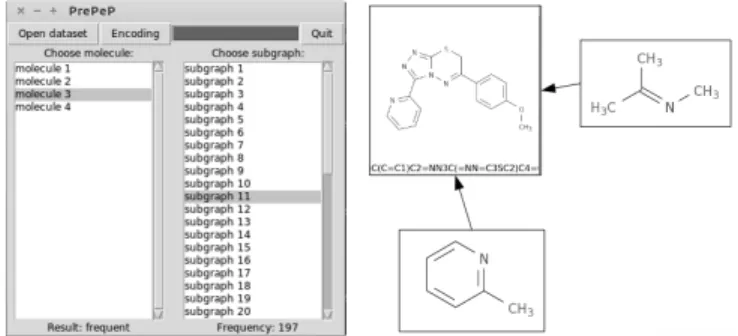
A screen shot of the interface can be seen in Figure 5: molecules to be predicted are shown in the left column. For each molecule predicted as FH, such as molecule 3 in this case, the right-hand column lists the discriminative subgraphs present in this molecule. Subgraphs are sorted by how often they were part of the result set of the mining operation, in descending order. Selecting a molecule visualizes it using OpenBabel, selecting a subgraph indicates its frequency in result sets at the bottom of the right-hand column, and visualizes the subgraph.

Figure 5: Screen shot of PrePeP’s interface.

8

CONCLUSIONS AND PERSPECTIVES

The experimental results validate our approach and our design choices. As we have shown on the FH/iFH data set, it is indeed possible to build a model that predicts FHs with good accuracy, and, more importantly, recovers a large amount of the FHs in the data. Our results also show that our model is a clear improvement over the structural alerts currently in use, particularly w.r.t. dark chemi-cal matter, on which we have significantly better results. Using a model that is not a black box allows us to present an explanation for the prediction to experts, facilitating acceptance and adding to scientific knowledge.

In its current form, PrePeP is ready for use but has some limita-tions. As discussed throughout the experimental evaluation, having used a data set evaluated on AlphaScreen assays seems to limit PrePeP’s predictive power when it comes to compounds that show frequent activity in other kinds of assays. This is not a problem per se since we can extend our prototype with subgraphs and predictive models derived from data stemming from other types of bioassays. In that case, PrePeP will contain several predictive modules, each of which can be used to predict whether a compound is FH or not, depending on the assay type the expert is interested in, with the option to perform a consensus prediction using all modules. In practical terms, however, this requires extensive exploration of PubChem to create appropriate data – an important reason for our using the AlphaScreen data set is that it is already available in curated form.

Related to this question is how one defines frequent hitters in the first place. In the work of Baell et al., any compound showing activity in two or more out of six assays was considered a frequent hitter. In their critique, Capuzzi et al. adopted the same threshold, and we therefore as well. It is not clear that this is an appropriate definition, however, and characterizing FHs in terms of their activ-ity percentage might be more informative. Changing the problem setting in this way brings us into actual QSAR territory and with regression arguably a more difficult problem setting than classifi-cation, the effectiveness of our method is unclear. Addressing this problem would also require extensive additional data acquisition. The parameters we have chosen for the prototype – top-100 subgraphs, three percent minimum size for decision tree leaves, two hundred samples – were selected as a result of the trade-off of running times and performance on the FH/iFH data set but it is not clear that they are the best choices in general terms. As a comparison, there were 480 PAINS alerts proposed in [6]. As we extend our approach to new data, it is possible that we will have to adjust those parameter values, or make them data-dependent.

Finally, our evaluations so far have been performed entirely in silico. To support our results, experimental biological assays are necessary, i.e. classifying new molecules and testing those classified as FH in multiple assays to verify their activity. This task requires deployment at our chemist partners to gather hands-on experience. Even for the first two aspects, however, strong expertise and knowledge in medicinal chemistry is needed, and we will address them in close cooperation between the involved computer science and medicinal chemistry laboratories. We intend nevertheless to make PrePeP available to the wider community as soon as possible and exploit their feedback. One option that we have explored but not yet implemented consists of giving experts feedback options, e.g. rejecting predictions or supposedly discriminative subgraphs. This will require a more elaborate interface and user tests, which cannot be outsourced to non-expert users. In addition, to take feedback into account, PrePeP will need to become much more reactive, moving away from the off-line mining and learning that it currently performs.

REFERENCES

[1] 2017. The Open Source Chemistry Toolbox. (dec 2017). https://openbabel.org [2] 2017. Public database of chemical molecules and their activities against biological

assays. (2017). https://pubchem.ncbi.nlm.nih.gov/about.html

[3] 2017. RDKit: Open-Source Cheminformatics. (2017). http://www.rdkit.org [4] Courtney Aldrich, Carolyn Bertozzi, Gunda I Georg, Laura Kiessling, Craig

Lindsley, Dennis Liotta, Kenneth M Merz Jr, Alanna Schepartz, and Shaomeng Wang. 2017. The ecstasy and agony of assay interference compounds. (2017). [5] Pieter Swart et al. Aric Hagberg, Dan Schult. 2017. Python package for the

creation, manipulation, and study of the structure, dynamics, and functions of complex networks. (dec 2017). https://networkx.github.io

[6] Jonathan Baell and Georgina Holloway. 2010. New substructure filters for removal of pan assay interference compounds (PAINS) from screening libraries and for their exclusion in bioassays. Journal of Medicinal Chemistry 53(7) (2010), 2719– 2740.

[7] Jonathan B Baell. 2016. Feeling nature’s PAINS: Natural products, natural product drugs, and pan assay interference compounds (PAINS). Journal of natural products 79, 3 (2016), 616–628.

[8] Jonathan B Baell and Walters Michael A. 2015. Chemical con artists foil drug discover. Nature 7519, 513 (2015), 481–483.

[9] M. R. Berthold, N. Cebron, T. R. Dill, F.and Gabriel, T. Kötter, T. Meinl, C. Ohl, P.and Sieb, K. Thiel, and B. Wiswedel. 2007. KNIME: The Konstanz Information Miner. Springer, Chapter Studies in Classification, Data Analysis, and Knowledge Organization (GfKL 2007).

[10] BIOVIA. 2017. BIOVIA Pipeline Pilot. (2017). http://accelrys.com/products/ collaborative-science/biovia-pipeline-pilot/

[11] BIOVIA. 2017. CTfile Formats. (2017). http://accelrys.com/products/ collaborative-science/biovia-draw/ctfile-no-fee.html

[12] N. Bosc, B. Wroblowski, C. Meyer, and P. Bonnet. 2017. Prediction of Protein Kinase-Ligand Interactions through 2.5D Kinochemometrics. J. Chem Inf Model. 57, 1 (2017), 93–101.

[13] Leo Breiman. 1996. Bagging Predictors. Machine Learning 24, 2 (1996), 123–140. [14] Leo Breiman, Jerome Friedman, Charles J. Stone, and R.A. Olshen. 1984.

Classifi-cation and Regression Trees. Chapman & Hall, New York. 358 pages.

[15] Björn Bringmann, Albrecht Zimmermann, Luc De Raedt, and Siegfried Nijssen. 2006. Don’t Be Afraid of Simpler Patterns. In 10th European Conference on Principles and Practice of Knowledge Discovery in Databases, Johannes Fürnkranz, Tobias Scheffer, and Myra Spiliopoulou (Eds.). Springer, 55–66.

[16] Matthieu Brucher. 2017. Library of Machine Learning tools in Python. (dec 2017). http://scikit-learn.org

[17] Stephen J Capuzzi, Eugene N Muratov, and Alexander Tropsha. 2017. Phantom PAINS: Problems with the Utility of Alerts for Pan-Assay INterference Com-poundS. Journal of chemical information and modeling 57, 3 (2017), 417–427. [18] Corinna Cortes and Vladimir Vapnik. 1995. Support-vector networks. Machine

learning 20, 3 (1995), 273–297.

[19] John G Cumming, Andrew M Davis, Sorel Muresan, Markus Haeberlein, and Hongming Chen. 2013. Chemical predictive modelling to improve compound quality. Nature reviews Drug discovery 12, 12 (2013), 948.

[20] Jayme L Dahlin, J Willem M Nissink, Jessica M Strasser, Subhashree Francis, LeeAnn Higgins, Hui Zhou, Zhiguo Zhang, and Michael A Walters. 2015. PAINS in the assay: chemical mechanisms of assay interference and promiscuous enzymatic inhibition observed during a sulfhydryl-scavenging HTS. Journal of medicinal chemistry 58, 5 (2015), 2091–2113.

[21] Richard Eglen, Terry Reisine, Philippe Roby, Nathalie Rouleau, Chantal Illy, Roger Bosse, and Martina Bielefeld. 2008. The Use of AlphaScreen Technology in HTS: Current Status. Journal of Current Chemical Genomics 1 (2008), 2–10. [22] J. M. Gally, S. Bourg, Q. T. Do, S. Aci-Sèche, and P. Bonnet. 2017. VSPrep: A

General KNIME Workflow for the Preparation of Molecules for Virtual Screening. Molecular Informatics 36 (2017).

[23] Rajarshi Guha. 2008. On the interpretation and interpretability of quantitative structure–activity relationship models. Journal of computer-aided molecular design 22, 12 (2008), 857–871.

[24] Daylight Chemical Information Systems, Inc. [n. d.]. Simplified Molecular Input Line Entry System. ([n. d.]). http://www.daylight.com/smiles/index.html [25] Akihiro Inokuchi and Takashi Washio. 2008. A fast method to mine frequent

subsequences from graph sequence data. In Data Mining, 2008. ICDM’08. Eighth IEEE International Conference on. IEEE, 303–312.

[26] Swarit Jasial, Ye Hu, and Jürgen Bajorath. 2017. How frequently are pan-assay interference compounds active? Large-scale analysis of screening data reveals diverse activity profiles, low global hit frequency, and many consistently inactive compounds. Journal of Medicinal Chemistry 60, 9 (2017), 3879–3886. [27] Ulf Johansson, Cecilia Sönströd, Ulf Norinder, and Henrik Boström. 2011.

Trade-off between accuracy and interpretability for predictive in silico modeling. Future medicinal chemistry 3, 6 (2011), 647–663.

[28] Michihiro Kuramochi and George Karypis. 2001. Frequent subgraph discovery. In Data Mining, 2001. ICDM 2001, Proceedings IEEE international conference on. IEEE, 313–320.

[29] Sylvain Lozano, Guillaume Poezevara, Marie-Pierre Halm-Lemeille, Elodie Lescot-Fontaine, Alban Lepailleur, Ryan Bissell-Siders, Bruno Cremilleux, Sylvain Rault, Bertrand Cuissart, and Ronan Bureau. 2010. Introduction of jumping fragments in combination with QSARs for the assessment of classification in ecotoxicology. Journal of chemical information and modeling 50, 8 (2010), 1330–1339. [30] Thomas Mendgen, Christian Steuer, and Christian D Klein. 2012. Privileged

scaffolds or promiscuous binders: a comparative study on rhodanines and related heterocycles in medicinal chemistry. Journal of medicinal chemistry 55, 2 (2012), 743–753.

[31] Jean-Philippe Métivier, Alban Lepailleur, Aleksey Buzmakov, Guillaume Poeze-vara, Bruno Crémilleux, Sergei O Kuznetsov, Jérémie Le Goff, Amedeo Napoli, Ronan Bureau, and Bertrand Cuissart. 2015. Discovering structural alerts for mutagenicity using stable emerging molecular patterns. Journal of chemical information and modeling 55, 5 (2015), 925–940.

[32] Shinichi Morishita and Jun Sese. 2000. Transversing itemset lattices with statis-tical metric pruning. In Proceedings of the 19th ACM SIGMOD-SIGACT-SIGART symposium on Principles of database systems. 226–236.

[33] Kathryn M Nelson, Jayme L Dahlin, Jonathan Bisson, James Graham, Guido F Pauli, and Michael A Walters. 2017. The essential medicinal chemistry of cur-cumin: miniperspective. Journal of medicinal chemistry 60, 5 (2017), 1620–1637. [34] Siegfried Nijssen and Joost Kok. 2006. Frequent subgraph miners: runtimes don’t say everything. In Proceedings of the Workshop on Mining and Learning with Graphs. 173–180.

[35] Siegfried Nijssen and Joost N Kok. 2004. A quickstart in frequent structure mining can make a difference. In Proceedings of the tenth ACM SIGKDD international

PrePeP – Identification and Characterization of PAINS KDD ’18, August 19–23, 2018, London, United Kingdom

conference on Knowledge discovery and data mining. ACM, 647–652.

[36] Martin Pouliot and Stephane Jeanmart. 2015. Pan Assay Interference Compounds (PAINS) and Other Promiscuous Compounds in Antifungal Research: Miniper-spective. Journal of medicinal chemistry 59, 2 (2015), 497–503.

[37] Marco Tulio Ribeiro, Sameer Singh, and Carlos Guestrin. 2016. "Why Should I Trust You?": Explaining the Predictions of Any Classifier. In 22nd ACM SIGKDD International Conference on Knowledge Discovery and Data Mining. ACM, 1135– 1144.

[38] Jürgen Schmidhuber. 2015. Deep learning in neural networks: An overview. Neural networks 61 (2015), 85–117.

[39] Sanjay Joshua Swamidass, Jonathan H. Chen, Jocelyne Bruand, Peter Phung, Liva Ralaivola, and Pierre Baldi. 2005. Kernels for small molecules and the prediction of mutagenicity,toxicity and anti-cancer activity. 359–368.

[40] Natasha Thorne, Douglas S Auld, and James Inglese. 2010. Apparent activity in high-throughput screening: origins of compound-dependent assay interference. Current opinion in chemical biology 14, 3 (2010), 315–324.

[41] Tihomir Tomašić and Lucija Peterlin Mašič. 2012. Rhodanine as a scaffold in drug discovery: a critical review of its biological activities and mechanisms of target modulation. Expert opinion on drug discovery 7, 7 (2012), 549–560. [42] David J Wood, David Buttar, John G Cumming, Andrew M Davis, Ulf Norinder,

and Sarah L Rodgers. 2011. Automated QSAR with a hierarchy of global and local models. Molecular informatics 30, 11-12 (2011), 960–972.

[43] Marc Wörlein, Thorsten Meinl, Ingrid Fischer, and Michael Philippsen. 2005. A quantitative comparison of the subgraph miners MoFa, gSpan, FFSM, and Gaston. In European Conference on Principles of Data Mining and Knowledge Discovery. Springer, 392–403.

[44] Xifeng Yan and Jiawei Han. 2002. gSpan: Graph-Based Substructure Pattern Mining. In ICDM. IEEE Computer Society, 721–724.

[45] Jeremy J Yang, Oleg Ursu, Christopher A Lipinski, Larry A Sklar, Tudor I Oprea, and Cristian G Bologa. 2016. Badapple: promiscuity patterns from noisy evidence. Journal of cheminformatics 8, 1 (2016), 29.

[46] Albrecht Zimmermann, Björn Bringmann, and Ulrich Rückert. 2010. Fast, Effec-tive Molecular Feature Mining by Local Optimization. In ECML/PKDD (3) (Lecture Notes in Computer Science), José L. Balcázar, Francesco Bonchi, Aristides Gionis, and Michèle Sebag (Eds.), Vol. 6323. Springer, 563–578.

APPENDIX

Table 4: Evaluation of the performance of the majority vote of different classifiers for different feature sets and different ratios of FHs and iFHs in the test data

Setting Algorithm Features Accuracy AUC score Precision Recall avg σ avg σ avg σ avg σ Balanced Random Forests subgraphs 37.72 2.49 0.3772 0.0249 0.4296 0.0158 0.7544 0.0498

numeric 81.67 2.92 0.8167 0.0292 0.855 0.0318 0.7633 0.0457 subgraphs+numeric 83.94 15.93 0.8394 0.1593 0.9024 0.1641 0.8144 0.0323 SVM subgraphs 78.5 16.8 0.785 0.168 0.9384 0.1949 0.67 0.0472 numeric 51.56 0.78 0.5156 0.0078 0.8667 0.322 0.0322 0.0143 subgraphs+numeric 52.22 1.26 0.5222 0.0126 0.8667 0.322 0.0456 0.0237 Naive Bayes subgraphs 61.83 16.59 0.6183 0.1659 0.9244 0.2392 0.3367 0.0832 numeric 68.83 2.32 0.6883 0.0232 0.6664 0.0257 0.7578 0.0335 subgraphs+numeric 68.67 16.32 0.6867 0.1632 0.9298 0.2132 0.4744 0.0859 Logistic Regression subgraphs 42.06 16.18 0.4206 0.1618 0.4824 0.1823 0.7411 0.0392 numeric 82.83 3.84 0.8283 0.0384 0.8283 0.0493 0.8311 0.0412 subgraphs+numeric 77.78 12.73 0.7778 0.1273 0.7685 0.1177 0.8467 0.0339 Stochastic Gradient subgraphs 38.56 2.69 0.3856 0.0269 0.4349 0.0166 0.7711 0.0537 Descent numeric 71.22 2.59 0.7122 0.0259 0.7154 0.0465 0.7156 0.0655 subgraphs+numeric 71.39 3.4 0.7139 0.034 0.7103 0.04 0.7256 0.0359 Slight Random Forests subgraphs 6.93 0.31 0.3811 0.0168 0.0708 0.0029 0.7622 0.0336 imbalance numeric 85.79 1.16 0.8133 0.0172 0.3656 0.0245 0.7589 0.0287 subgraphs+numeric 85.86 27.55 0.8387 0.1508 0.6068 0.1901 0.8144 0.024 SVM subgraphs 87.85 28.56 0.7817 0.1485 0.9067 0.2949 0.6633 0.0359

numeric 91.18 0.21 0.517 0.0113 0.8708 0.1889 0.0344 0.0225 subgraphs+numeric 91.29 0.28 0.5231 0.0148 0.8889 0.1712 0.0467 0.0295 Naive Bayes subgraphs 84.8 28.13 0.6139 0.1276 0.905 0.3005 0.3278 0.0911 numeric 63.29 1.45 0.6896 0.0214 0.1667 0.0095 0.7589 0.0396 subgraphs+numeric 85.8 28.2 0.6759 0.1336 0.8737 0.2881 0.4533 0.0828 Logistic Regression subgraphs 6.67 0.28 0.3667 0.0155 0.0683 0.0027 0.7333 0.031

numeric 81.62 0.79 0.8204 0.0193 0.3089 0.0141 0.8256 0.0363 subgraphs+numeric 71.81 22.46 0.7759 0.1208 0.2622 0.0688 0.8467 0.0286 Stochastic Gradient subgraphs 6.89 0.36 0.3789 0.0196 0.0704 0.0034 0.7578 0.0391 Descent numeric 71.66 4.76 0.7056 0.0189 0.2008 0.0223 0.6922 0.0505 subgraphs+numeric 71.8 4.38 0.7059 0.0241 0.201 0.0219 0.6911 0.0725 Severe Random Forests subgraphs 0.74 0.04 0.3728 0.0178 0.0074 0.0004 0.7456 0.0357 imbalance numeric 87.11 0.58 0.8189 0.0256 0.0566 0.0042 0.7656 0.0517 subgraphs+numeric 86.71 30.18 0.8383 0.1493 0.1681 0.0616 0.8089 0.0347 SVM subgraphs 89.77 31.31 0.7833 0.1593 0.9007 0.3141 0.6667 0.0392 numeric 99 0.03 0.5159 0.0096 0.4054 0.1554 0.0322 0.0192 subgraphs+numeric 98.99 0.02 0.5213 0.0112 0.3757 0.1309 0.0433 0.0225 Naive Bayes subgraphs 89.45 31.33 0.6222 0.173 0.9003 0.3153 0.3444 0.0856 numeric 62.73 0.67 0.6908 0.0361 0.0198 0.0019 0.7556 0.0699 subgraphs+numeric 89.39 31.28 0.6709 0.173 0.6487 0.2299 0.4433 0.074 Logistic Regression subgraphs 0.73 0.05 0.3683 0.023 0.0073 0.0005 0.7367 0.046 numeric 81.34 0.49 0.8199 0.0118 0.0424 0.0014 0.8267 0.0241 subgraphs+numeric 71.56 24.76 0.7788 0.12 0.0364 0.0108 0.8433 0.0231 Stochastic Descent subgraphs 0.74 0.04 0.3756 0.0213 0.0075 0.0004 0.7511 0.0426 Descent numeric 72.95 4.71 0.7078 0.0331 0.0249 0.0023 0.6856 0.0986 subgraphs+numeric 72.63 4.43 0.7116 0.032 0.0252 0.0038 0.6967 0.0759