Family income and child health in the UK

HAL Id: halshs-00794729

https://halshs.archives-ouvertes.fr/halshs-00794729

Preprint submitted on 26 Feb 2013

HAL is a multi-disciplinary open access

archive for the deposit and dissemination of sci-entific research documents, whether they are pub-lished or not. The documents may come from teaching and research institutions in France or abroad, or from public or private research centers.

L’archive ouverte pluridisciplinaire HAL, est destinée au dépôt et à la diffusion de documents scientifiques de niveau recherche, publiés ou non, émanant des établissements d’enseignement et de recherche français ou étrangers, des laboratoires publics ou privés.

Family income and child health in the UK

Bénédicte H. Apouey, Pierre-Yves Geoffard

To cite this version:

Bénédicte H. Apouey, Pierre-Yves Geoffard. Family income and child health in the UK. 2013. �halshs-00794729�

WORKING PAPER N° 2013 – 03

Family income and child health in the UK

Bénédicte Apouey

Pierre-Yves Geoffard

JEL Codes : I1

Keywords: Child health; Family income; Gradient

P

-

S

E

48, BD JOURDAN – E.N.S. – 75014 PARIS TÉL. : 33(0) 1 43 13 63 00 – FAX : 33 (0) 1 43 13 63 10

www.pse.ens.fr

CENTRE NATIONAL DE LA RECHERCHE SCIENTIFIQUE – ECOLE DES HAUTES ETUDES EN SCIENCES SOCIALES

Family income and child health in the UK

B´en´edicte Apoueya_{, Pierre-Yves Geoffard}b

February 25, 2013

a_{Paris School of Economics - CNRS, 48, Boulevard Jourdan, 75014 Paris, France.}

E-mail address: benedicte.apouey@parisschoolofeconomics.eu.

b_{Paris School of Economics - CNRS, 48, Boulevard Jourdan, 75014 Paris, France.}

E-mail address: geoffard@pse.ens.fr.

Send all correspondence to: B´en´edicte Apouey

Paris School of Economics 48, Boulevard Jourdan 75014 Paris France Voice: 33-1-43-13-63-07 Fax: 33-1-43-13-63-55 E-mail: benedicte.apouey@parisschoolofeconomics.eu.

Abstract

Recent studies examining the relationship between family income and child health in the UK have produced mixed findings. We re-examine the income gradient in child general health and its evolution with child age in this country, using a very large sample of British children. We find that there is no correlation between income and child general health at ages 0-1, that the gradient emerges around age 2 and is constant from age 2 to age 17. In addition, we show that the gradient remains large and significant when we try to address the endogeneity of income. Furthermore, our results indicate that the gradient in general health reflects a greater prevalence of chronic conditions among low-income children and a greater severity of these conditions. Taken together, these findings suggest that income does matter for child health in the UK and may play a role in the intergenerational transmission of socioeconomic status.

JEL classification: I1

Keywords: Child health; Family income; Gradient

Acknowledgments

Data from the FACS were supplied by the ESRC Data Archive. Neither the original collectors of the data nor the Archive bear any responsibility for the analysis or interpre-tations presented here. We would like to thank two anonymous referees, Hugh Gravelle, Gabriel Picone, Jennifer Stewart, Michael Wolfson, and participants to the Health Eco-nomics seminar at the University of South Florida (2011), the 45th Annual Conference of the Canadian Economics Association (2011), and the CES-HESG workshop in Aix-en-Provence (2012) for their constructive comments.

1

Introduction

A large amount of literature shows a positive correlation between socioeconomic status and health in adulthood (Adler et al., 1994; Deaton and Paxson, 1998; Deaton and Paxson, 1999; Van Doorslaer et al., 1997; Wilkinson and Marmot, 2003). Recent research initiated by Case et al. (2002) investigates whether the gradient in general health observed in adulthood has antecedents in childhood. Understanding the determinants of child health is important because health in childhood affects human capital accumulation, and health and labor market status in adulthood (Currie, 2008). Findings firmly establish that family income is positively related to children’s general health in Australia (Khanam et al., 2009), Canada (Currie and Stabile, 2003), Germany (Reinhold and J¨urges, 2011), and the US (Case et al., 2002; Condliffe and Link, 2008). Moreover, the correlation between family income and children’s general health strengthens as children grow older in Canada and the US, meaning that the disadvantages associated with parental income accumulate as children age (Case et al., 2002; Currie and Stabile, 2003). These authors argue that the steepening of the gradient with age can be due to two mechanisms: (1) either children from poorer families are more likely to be subject to health shocks than their wealthier counterparts (prevalence effect), or (2) poorer children are less able to respond to health shocks, and so health shocks are more severe for them (severity effect). The distinction between these two mechanisms is important because they have different implications from a policy perspective: the first mechanism implies that the gradient may be reduced by addressing the reasons why poorer children are more likely to get chronic conditions, whereas the second mechanism means that a policy should improve access to palliative care for poorer children. In the US, the strengthening of the gradient is due to a combination of a prevalence and a severity effects (Case et al., 2002), whereas in Canada, it is only due to a prevalence effect (Currie and Stabile, 2003).

Findings on the gradient in general health for British children are not firmly estab-lished. Currie et al. (2007) and Case et al. (2008) analyze the evolution of the gradient as children grow older, using cross-sectional data from the Health Survey for England (HSE), the same variables, and the same methods. Specifically, they estimate the gradient for four age groups (children ages 0-3, 4-8, 9-12, 13-17) and compare the estimates between the age groups to depict the evolution of the gradient with age. In spite of these similarities, their conclusions are different. Currie et al. (2007) highlight that there is a gradient in general

health, that it increases between 0-3 and 4-8 and stops increasing afterwards, using six waves of the HSE. In contrast, Case et al. (2008) conclude that the gradient in general health does increase with age from birth to age 12, using three additional years of data from the HSE. In addition, Propper et al. (2007) suggest that when maternal health and behaviors are included, there is almost no correlation between family income and child health, for a cohort of British children less than 7 years of age. This means that the gradient may not reflect any causal effect of family income on child health.

The previous literature on the UK uses relatively small datasets, which could explain why the results are somewhat contradictory. A larger sample of British children may shed more light on the gradient in general health. In addition, the previous literature on the UK investigates the evolution of the gradient in general health using four age groups, which makes it impossible to examine the turning points in the evolution of the gradient with age. We suggest to compare the gradient between ages, instead of age groups, to get a precise description of the evolution of the general health/income relationship with age. Finally, in a small sample like the HSE, it is not possible to study the role of rare chronic conditions in the general health gradient: the analysis of rare chronic conditions requires large sample sizes.

This paper re-examines the general health/income gradient in childhood in the UK, using a large sample of approximately 78,000 children drawn from the Family and Children Survey (FACS). First, we exploit the large sample size of the FACS to investigate the evolution of the gradient with child age in a more detailed manner. Specifically, we estimate the effect of income on health separately for children of each age, instead of each age group. Second, we examine whether the association between family income and child health could represent causality running from income to child health, as opposed to reverse causality or the omission of third factors. We adopt two strategies. On the one hand, we take advantage of the information we have on the influence of child health on family income in the FACS, to reduce reverse causation. As far as we are aware, we are the first to deal with this issue in a precise manner. On the other hand, we expand on the number of controls to address the omission of factors. Third, we examine the role of specific health problems, in particular some rare chronic conditions, Special Educational Needs, and the attention deficit hyperactivity disorder (ADHD), in the gradient in general health. Fourth, we investigate the channels through which family income could have an impact on child health, focusing on the use of health care services, housing conditions, nutrition,

and clothing.

We find that there is a very small or negligible effect of family income on general health for children ages 0-1 and a large and significant effect for children above 2. In addition, the gradient remains constant as children grow older, from age 2 to age 17. This description of the gradient is very different from that given in the earlier literature on the UK, which highlights an increase in the gradient with age between birth and age 8 at least. We also show that our results are robust to various procedures that mitigate the bias due to the endogeneity of income. The paper also finds that the gradient in general health could be explained both by the prevalence and severity of specific health problems among low-income children, which implies that policies should address the reasons why low-low-income children are more likely to obtain specific health problems and why the severity of these specific problems depends on income. Finally, we show that the effect of family income on child health is not accounted for by differences in the use of health care services, housing conditions, nutrition, and clothing between low and high-income children. However, hous-ing conditions, nutrition, and clothhous-ing do have a large independent effect on child general health.

The rest of the paper proceeds as follows. In Section 2, we begin by discussing the contributions of the previous literature and highlight the originality of our approach. Section 3 provides an overview of the data. Section 4 investigates in details the evolution of the gradient and discusses the endogeneity of income. Section 5 focuses on the role of specific health problems in the gradient in general health. Section 6 examines whether the use of health care services, housing conditions, nutrition, and clothing are important channels through which family income influences child health. The Section also contains additional results on the role of maternal education in child health. Lastly, Section 7 offers some concluding remarks.

2

Background

We first briefly present the previous literature, focusing on the four aspects of the gradient that we are interested in: whether there is a correlation between income and child general health, whether this correlation changes with child age, whether the gradient represents a causal effect of income on general health and whether specific health problems, such as

chronic conditions, play a role in the gradient in general health. Developed countries other than the UK

Case et al. (2002) show that child general health is positively related to family income and that this relationship becomes more pronounced as children grow older in the US, using cross-sectional data from the National Health Interview Survey. Interestingly, the gradient probably reflects a causal effect of family income on child general health in the US.

Currie and Stabile (2003) demonstrate that the results of Case et al. (2002) also hold in Canada. In addition, they provide evidence that the gradient increases with age because low-income children are more likely to be subject of health shocks.

Khanam et al. (2009) investigate the gradient in Australia, using the first two waves of the Longitudinal Study of Australian Children. They find that there is a gradient that strengthens with age, when similar covariates to Case et al. (2002) are included. However, when they include richer sets of controls to address the endogeneity of income, the gradient disappears. These results suggest that in Australia the gradient may not reflect any causal effect of income on health, but could be due to the omission of factors.

Finally, Reinhold and J¨urges (2011) show that the gradient in Germany is as strong as in the US but that the disadvantages associated with parental income do not accumulate as children grow older.

The UK

In contrast with the clear findings for other developed countries, previous results on the gradient in general health in the UK are not firmly established. Patrick West argues that there is a strong socioeconomic gradient in childhood, but that it decreases or virtually disappears in youth, i.e. from age 12. Youth would be a period of relative equality in health with respect to self-rated health (West, 1988), mortality, symptoms of acute illness, non-fatal accidents, and injuries (West, 1988, 1997). West’s approach is mainly descriptive and it raises the question of the extent to which the association between socioeconomic status and child health reflects a causal effect of socioeconomic status as opposed to the endogeneity of socioeconomic status. Our paper investigates that point.

Currie et al. (2007) and Case et al. (2008) also explore the evolution of the gradient with age, in an econometric framework. These two papers use similar approaches but draw different conclusions. They both use cross-sectional data from the Health Survey

for England (HSE) and examine the gradient using four age groups: children ages 0-3, 4-8, 9-12 and 13-15. The authors quantify the gradient for each of these age groups and compare the gradient estimates between the groups, to depict the evolution of the gradient with age. Currie et al. (2007) use data from the 1997-2002 HSE, which corresponds to approximately 14,000 children. They find that there is a significant family income gradient in child general health for each age group, and that this gradient increases between ages 0-3 and 4-8 and decreases afterwards. Case et al. (2008) re-examine these findings using the same method and variables but an expanded sample from the HSE, by adding three years of data, which corresponds to approximately 20,000 children. In contrast with Currie et al. (2007), they conclude that the income-general health gradient increases with age between birth and age 12. In spite of their similarities, the papers by Currie et al. (2007) and Case et al. (2008) reach different conclusions. We think that a larger dataset might help get more stable results. In addition, these two papers use four age groups, which makes it impossible to get a precise description of the evolution of the gradient with age. Knowing at which age the gradient strengthens is important because it indicates the optimal age at which policies aimed at reducing social inequalities in health should be implemented. In this perspective, we suggest examining the evolution of the gradient between ages, instead of age groups.

Kruk (2010) analyzes the role of chronic conditions in the gradient in general health. She investigates whether poor children are more likely to obtain chronic conditions (preva-lence effect) and whether chronic conditions are more severe for poor children (severity effects). Kruk (2010) uses the first three waves of the Millennium Cohort Study (MCS), which corresponds to approximately 13,000 children less than 6. She examines the preva-lence effect for children ages 2-3 (wave 2) and 5-6 (wave 3) and the severity effect for children ages 5-6 (wave 3). She shows that there are both a prevalence and a severity effect for young British children. However, as pointed out by Case et al. (2008), it is not possible to get precise estimates of the role of rare chronic conditions with small sample sizes. Our paper tries to fill this gap in the literature.

Following Burgess et al. (2004), Propper et al. (2007) investigate whether the gradient represents a causal effect of income on health. They use data from the Avon Longitudinal Study of Parents and Children (ALSPAC), which contains from 4,000 to 11,000 children (depending on specifications) below 7 years of age. When basic sets of controls are in-cluded, the authors find a positive correlation between family income and child health,

but no evidence of an increase of the gradient between birth and age 7. To mitigate the problem of the endogeneity of income due to observed factors, they then expand the num-ber of controls. When they include parental behaviors and health, the gradient almost disappears. This finding thus casts doubts on the existence of a causal effect of family income on child health. It also raises the question of whether this result also holds for children above 7 and for a larger sample of children. Our paper provides precise answers to these questions.

2.2 Our approach

In this article, we use the Families and Children Study (FACS) to explore the effect of income on health in the UK. These data have a number of interesting characteristics compared to the ALSPAC, MCS, and HSE used in the previous literature. Table 1 presents a brief comparison of the FACS data with these datasets. First, the sample size of the FACS is much larger, for each age. Second, the FACS contains children of all ages, from 0 to 17. Third, parents always report their children’s health, whatever their age is, so the child general health measure is consistent across ages, unlike in the HSE. Fourth, household members report their exact income level and not income in brackets, which reduces measurement error in the income variable. Fifth, the FACS data are longitudinal and we could thus compute the average income for each household. Average income is less likely to be measured with error than current income. Taken together, these characteristics of the data enable us to get more precise estimates of the child health/income gradient than the previous literature.

[Insert Table 1 here]

In this paper, we exploit the large sample size of the FACS to investigate the existence and evolution of the gradient in childhood. Specifically, we estimate the gradient in general health at each age, instead of each age group.

We also try to explore whether the correlation between family income and child general health represents a causal effect of income on health, as opposed to reverse causation and the omission of third factors. To do that, we take advantage of the FACS data and eliminate from the sample the households for which we suspect a causal effect running from child health to family income. As far as we are aware, this constitutes an originality of this paper. In addition, to address the omission of third factors, we estimate augmented

models in which we include a large number of controls (Case et al., 2002; Khanam et al., 2009; Propper et al, 2007). However, note that despite our attempts, our models do not fully eliminate the endogeneity bias.

This paper also analyzes the role of specific health problems in the gradient in general health, focusing on the role of chronic conditions (including some rare conditions), Special Educational Needs, and ADHD. This focus on Special Educational Needs and ADHD represents an innovation for a study on the UK (Currie and Lin, 2007). We investigate whether low-income children are more likely to obtain specific health problems and whether these specific problems are more detrimental to their general health.

Finally, the paper investigates whether the use of health care services, housing con-ditions, nutrition, and clothing are channels through which family income translates into better child health.

3

The data

We use the 2001-2008 FACS to investigate the gradient in childhood in the UK. The FACS was formerly known as the Survey of Low Income Families, which started in 1999. It originally provided a new baseline survey of Britain’s lone-parent families and low-income couples with dependent children. Starting 2001, the survey was extended to include higher-income families, thereby yielding a complete sample of all British families (and the subsequent name change). We use all the available years of data from 2001. The data is a short panel with respondents being re-interviewed in subsequent waves.1

We focus on children who are dependent and who do not work. After elimination of missing values, the sample contains 78,541 observations.

Child good general health

Our main dependent variable is the general health of the child. It is generated by asking the respondent (who is generally the mother or the father of the child):

“(Since your baby was born/over the last 12 months) would you say (child’s name) health has been good, fairly good or not good?”

In our analysis, we use a dichotomous variable that equals one if the child is in good health and 0 otherwise.

1_{Before eliminating any observation with missing value, 11,601 children are “interviewed” only once,} 3,818 twice, 3,161 three times, 2,485 four times, 2,563 five times, 1,976 six times, 3,064 seven times, and 1,769 eight times.

Child specific health problems: Chronic conditions, Special Educational Needs and ADHD The FACS also contains information on whether the child has a number of following health problems, long-standing illnesses or disabilities. Specifically, parents are asked:

“Does (child’s name) have any standing illness or disability? By long-standing I mean anything that has troubled (child’s name) over a period of time or that is likely to affect (child’s name) over a period of time?”

If the question is answered in the positive, then parents are asked to indicate the kind of illness or disability the child has, from the following list: 1) Problem with arms, legs, hands, feet, back or neck; 2) Difficulty in seeing; 3) Difficulty in hearing; 4) Skin conditions, allergies; 5) Chest, breathing problem, asthma, bronchitis; 6) Heart, blood pressure or blood circulation problems; 7) Stomach, liver, kidney or digestive problems; 8) Diabetes; 9) Depression, bad nerves; 10) Mental illness, phobia, panics or other nervous problems; 11) Learning difficulties (or mental handicap); 12) Epilepsy; 13) Child congenital conditions; 14) Other health problems or disabilities. Most of these problems can be considered as chronic health conditions. We use a dummy variable for whether the child has any these chronic conditions and a series of dummy variables for whether the child has each of these conditions (except for the ones that are too rare in our sample). Note that the respondent to these questions on health problems is always one of the child’s parents (in most cases his mother), even for older children.

Information is also collected on whether the child was identified at school as having Special Educational Needs. This is a good indicator of child health, since the reason for being identified as having these needs are typically dyslexia, dyscalculia, dyspraxia, and ADHD. For our analyses, we also break out ADHD separately.

The mother’s and father’s health

The data contain the same health variables for the respondent and his partner. Using this information, we can find the mother and father’s general health and chronic conditions. We also use information on whether the mother smokes.

Income

The data contain a variable for the weekly income of the family in pounds, we adjust it using the 2005 CPI. Income is likely to be measured with error, which may bias our results. To reduce the measurement error, we average income over all the available years, provided that there are at least two years of data. In most of our estimations, we take

the logarithm of average income, to account for the non-linearity in the health/income relationship.

Summary statistics for the analysis sample are in Table 2. [Insert Table 2 here]

First description of the gradient

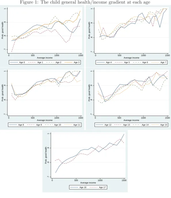
We first present evidence on the relationship between average family income and child general health, in the absence of any control. Figure 1 shows the probability that the child is in good health as a function of average family income, separately for children of each age. For children ages 0 and 1, the income gradient is positive but small. For children above 2, the income gradient is positive and larger. In addition, for children above 2, the gradient seems to remain constant with child age: we neither observe a strengthening nor a vanishing of the gradient as children grow older. This result contrasts with findings by West (1997) who shows using the 1991 British Census, that the gradient, which is strong until age 10, diminishes or vanishes for adolescents ages 11-19. Our findings also differ from previous results for the US which highlight a steepening of the gradient with child age (Case et al., 2002).

[Insert Figure 1 here]

4

The child general health/family income gradient

The correlation between income and health we have just highlighted could be due to the omission of parental, household, and child-specific characteristics. To address this concern, we run models that control for these characteristics. We examine both the existence of the income gradient and its evolution with age.

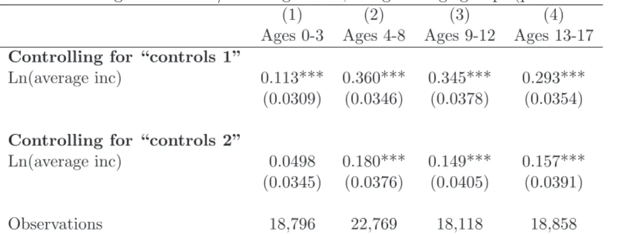
We first replicate the analysis of Case et al. (2002) and Currie and Stabile (2003) using the FACS data. Specifically, we estimate equations of child general health as a function of household income and controls, separately for four age groups (children ages 0-3, 4-8, 9-12 and 13-17), using probit models. We use two different sets of regressors, as in the previous literature. The first set of regressors, “controls 1”, includes a complete set of age and year dummies, the logarithm of household size, indicators for whether the respondent

is white, the child has a mother in the household, has a father in the household, and is male. The second set of regressors, “controls 2”, contains the first set of controls plus interaction terms between the mother’s and the father’s presence in the household and their education level and employment status.

Our results are presented in Table 3. When “controls 1” are included, the coefficient on income is positive and significant for all age groups, which means that children living in wealthier households are in better general health. However, in contrast with American and Canadian results, we do not observe any strengthening of the income gradient with child age. When controls for parents’ education and employment status are included, the income gradient disappears for children ages 0-3, but remains significant for children above 4. Again, there is no evidence that the gradient increases during childhood.

[Insert Table 3 here]

4.2 A precise description of the gradient

We now turn to a more precise description of the evolution of the income gradient with child age, by separately analyzing children of each age, instead of each age group. First, we examine the existence of the income gradient at each age, by estimating the following linear probability model:

G= α + β0Ln(average income) × Age 0 + β1Ln(average income) × Age 1

+... + β17Ln(average income) × Age 17

+Xγ + ǫ

(1)

where G is a dummy indicating that the child is in good general health, Ln(average income)× Age krepresents an interaction term between the logarithm of average income and age k, which equals the logarithm of average income if the child is k years old, and zero otherwise, X is a set of controls, and ǫ is the error term.

The estimates of β0, ...β17 and their confidence intervals give information on the

exis-tence of the gradient at each age: there is an income gradient in general health at age k if the lower bound of the confidence interval of βk is greater than zero.

G= α + χLn(average income)

+δ1Ln(average income) × Age 1 + δ2Ln(average income) × Age 2

+... + δ17Ln(average income) × Age 17

+Xγ + ǫ

(2)

In this equation, the effect of income on child health at age zero is the reference. The gradient at age k is significantly larger than the gradient at age zero if the lower bound of the confidence interval of δk is greater than zero.

Equations (1) and (2) are estimated using the two sets of regressors presented above (“controls 1” and “controls 2”). With the exception of the set of age dummies, all the controls are interacted with two-year age group dummies,2

to account for the possibility that they have different effects on child general health over childhood years.

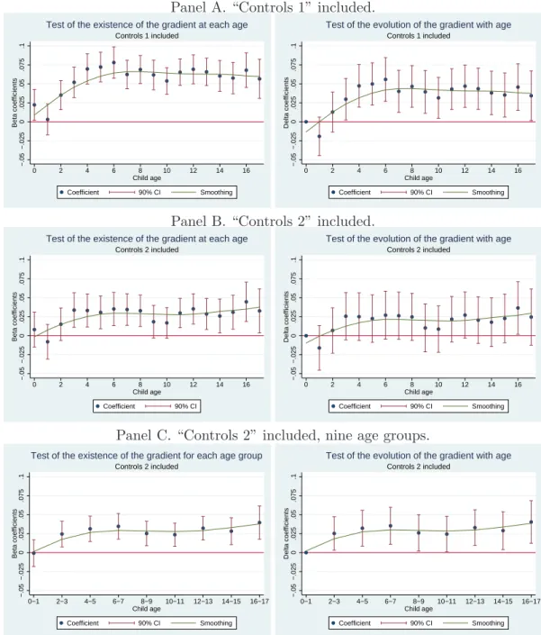
Panels A and B in Figure 2 represent the coefficients β0, ...β17 on the left graphs, and

δ1, ...δ17, on the right graphs, as a function of age, their 90% confidence intervals and a

nonparametric smoothing.

Figure 2, Panel A, graphs the results when “controls 1” are included. The top left graph indicates that the income gradient is significant at each age, except age 1. The graph also suggests that the gradient is either null or small at ages 0 and 1, that it increases between ages 1 and 3 and remains stable for children above 3. The top right graph shows that the gradient at ages 1 and 2 is not significantly different from the gradient at age 0, but that the gradient above 3 is significantly larger than at age 0.

Figure 2, Panel B, represents the coefficients of interest as a function of age, when additional controls for parental education and employment are included (“controls 2”). Comparing the left graph in Panel B with the left graph in Panel A indicates that the inclusion of these additional controls reduces the size of the gradient. However, the gradient is still significant for children of all ages when “controls 2” are included, except for ages 0, 1, 2, 9, and 10.

In Panel B, the confidence intervals of the estimated coefficients are large, which means that the coefficients are not precisely estimated. To improve the quality of the estimates, we re-run equations (1) and (2) using nine age groups, for children ages 0-1, 2-3, 4-5, 6-7, 8-9, 10-11, 12-13, 14-15, and 16-17. The new estimates on the interaction terms between

income and these age groups are reported in Panel C. The left graph in Panel C shows that the gradient is significant at all ages, except at ages 0-1. The right graph in Panel C provides some evidence of an emergence of the gradient in early childhood between 0 and 2. In addition, both graphs in Panel C suggest that the gradient is stable from age 2 to age 17. These findings contrast with those from the previous literature on the UK and other developed countries: Case et al. (2008) find that the gradient strengthens from birth to age 12 in the UK, using a smaller sample of British children and four age groups, whereas Case et al. (2002) and Currie and Stabile (2003) provide evidence of a continuous increase of the gradient from birth to age 17, in the US and Canada.

[Insert Figure 2 here]

4.3 The endogeneity of income

A key question is the extent to which the gradient we have just estimated represents a causal effect of income on child health as opposed to the endogeneity of income. In this section, we re-examine the existence of the gradient for the whole sample, the existence of the gradient at each age, and the evolution of the gradient across ages, when minimizing the endogeneity bias. We try to address the two sources of the endogeneity of income: reverse causation and the omission of third factors.

First, our previous estimates are biased by reverse causation if child health has an effect on family income, for instance if parents do not work or reduce their work hours because of their child health or if the household receives an allowance because of child disability. To contain reverse causation, we restrict the sample to households in which there is no child whose health influences family income. Specifically, we eliminate from the analysis sample households in which at least one of the children’s health prevents their parents from doing a paid job or from working as many hours as they would do otherwise,3

from looking for a job of 16 or more hours a week, and households who receive a disability living allowance (care or mobility) for a child.4

In total, we drop more than 10,000 observations.

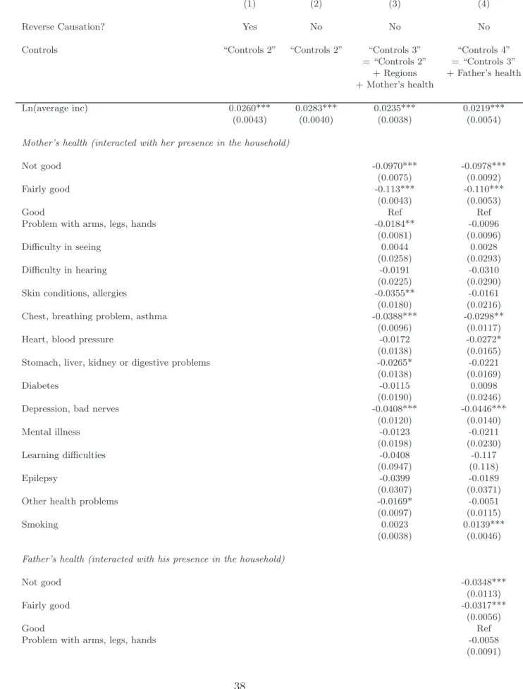
In addition, the estimates of the gradient presented above do not represent the causal effect of income on child health if important third factors are omitted. To minimize this bias, we expand the number of regressors and include controls for British regions and for the parents’ health. Indeed, articles by Khanam et al. (2009) and Propper et al. (2007)

3_{This piece of information is available from 2004 in the data.} 4_{This piece of information is available from 2004 in the data.}

suggest that parents’ health is an important determinant of child health, whose omission biases the gradient estimates.

The results are presented in Table 4. Column (1) contains the estimate of the income gradient, before the elimination of reverse causation, when “controls 2” are included. Column (2) contains the estimate of the gradient, when there is no reverse causation, and when “controls 2” are included. Comparing columns (1) and (2) suggests that the bias in the gradient estimate due to reverse causation is small. In columns (3) and (4), we expand the number of controls to address the omission of factors. When we include controls for the regions and the mother’s health (“controls 3”) in column (3), the coefficient on income decreases but remains very large and significant. This means that in the FACS, the correlation between family income and child health is not due to the omission of controls for the mother’s health.

The estimates also suggest that the effect of the mother’s health on child health is important; this is especially true for maternal mental problems. These findings confirm previous conclusions by Propper et al. (2007).

The inclusion of the father’s health in column (4) has a small impact on the coefficient on income, which means that the effect of the father’s health on child health is almost independent of the effect of income.

The inclusion of the father’s health implies a large reduction of the sample size, because the father’s health variables have many missing values. In addition, the inclusion of father’s health has a small effect on the correlation between income and health. For these two reasons, we will not include the father’s health in the models presented in the rest of the paper.

[Insert Table 4 here]

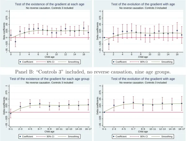
In further analysis, we investigate the existence of the gradient at each age and its evo-lution with child age, when reducing the endogeneity of income. Specifically, we eliminate reverse causation and then re-estimate equations (1) and (2), including either “controls 2” or “controls 3”. Figures 3 and 4 display the new estimates of the interaction terms between income and age, as a function of child age.

Findings from Figures 3 and 4 support previous results presented in Figure 2. First, Figure 4, Panel B, indicates that when controls for maternal health are included, there is a positive and significant gradient in childhood, except for infants ages 0 and 1. This results

contrasts with the conclusions of Propper et al. (2007) for the UK and Khanam et al. (2009) for Australia, who observe that the gradient (almost) disappears when maternal health is included, for young children ages 0-7. Second, regarding the evolution of the gradient with age, Figures 3 and 4 provide some evidence of an emergence of the gradient between ages 0 and 2 and prove that the gradient is stable between ages 2 to 17.

[Insert Figures 3 and 4 here]

4.4 Robustness checks

Our results show that there is no income gradient for children ages 0-1. This can seem surprising since a number of studies find that low income children are more likely to be born with low birth weight, and we know that low birth weight is associated with health problems. This apparent disconnect between our results on the one hand and the previous literature on the other hand could be due to the assumption we made that the effect of income on general health is log-linear. We thus examine whether there is a positive relationship between income and general health for young children, under a weaker assumption on the functional form of the effect of income on health.

Specifically, we use a series of dummies for income deciles instead of the logarithm of income. Table 5 contains the results of the regression of child health on the deciles, separately for children age 0 in column (1), age 1 in column (2), and ages 0 and 1 in column (3). The table does not show any significant correlation between income deciles and general health at ages 0 and 1. So the apparent disconnect between our finding on the absence of income gradient in early childhood and the literature on the impact of income on birth weight is not due to our assumption of log-linearity.

[Insert Table 5 here]

An alternative explanation for the disconnect between our results on the absence of any gradient at ages 0-1 and the previous literature on the gradient in birth weight is that the general health variable we use is not sensitive enough to pick up the health problems of very young children ages 0-1. Since this general health variable has been used by most of the recent literature in the gradient in childhood, this issue goes far beyond our sole article, and would require further investigation in the future.

We also check the robustness of our findings on the existence and stability of the gradient between ages 2 and 17 using other specifications. More precisely, we use either

the dichotomous general health variable (Good health vs Fairly good and Not good) or the general health variable with three categories (Not good, Fairly good, Good). We estimate the gradient for each age separately using 18 distinct models, using simple and ordered probit models. Supporting our previous findings, the results indicate that there is a positive and significant income gradient from age 2 to age 17.

In (ordered) probit models, it is not possible to test the evolution of the gradient with age by including a complete set of interaction terms between income and age, and examining their sign (Ai and Norton, 2003). In these non-linear models, testing the evolution of the gradient with age is tedious and requires to include one single interaction term between income and age at a time (see Norton et al., 2004, and the Inteff Stata command). Having this limitation in mind, we implement the test and find that the gradient is stable with age above 2.

5

The role of specific health problems

The previous section demonstrates that there is no gradient in general health at ages 0-1, that this gradient emerges in early childhood and remains stable from then on. We now turn to the role of specific health problems in the gradient in general health.

5.1 Prevalence and severity effects in static models

The gradient in general health can be explained by the prevalence and severity of some specific health problems, such as chronic conditions (Case et al., 2002). First, low-income children may be more likely to have specific health problems than high-income children (prevalence effect). Second, even if low-income children are not more likely to get specific health problems, the specific health problems they get may be more severe, compared to high-income children (severity effect). Equivalently, income may buffer the negative consequences of specific health problems.

We assess the importance of the prevalence effect using a series of linear probability models:

Si,t = α0+ α1Ln(average income)_i+ X_i,tδS+ ǫS_i,t (3)

where S indicates that the child has a specific health problem. The prevalence effect is captured by the coefficient α1, which indicates whether poorer children are more likely to

obtain specific health problems or not.

The importance of the severity effect is assessed by the following model:

Gi,t= φ0+φ1Ln(average income)_i+φ2S_i,t+φ3Ln(average income)_i×Si,t+X_i,tδG+ǫG_i,t (4)

where G indicates that the child is in good general health. The severity effect is given by the coefficient φ3: if φ3is positive and significant, income buffers the negative consequences

of the specific health problem on general health.

Equations (3) and (4) are estimated separately for the following specific health prob-lems: having any chronic condition, having each chronic condition, Special Educational Needs, and ADHD.

We treat having any chronic conditions and having each chronic condition on the one hand and Special Educational Needs and ADHD on the other hand separately. Indeed, chronic conditions are internally noted by the parents. In contrast, Special Educational Needs and ADHD are externally noted and diagnosed. The impact of income on internally diagnosed conditions is likely to be different from the impact of income on externally diag-nosed problems. For example, if children from high income families are less likely to have an objective Special Educational Need, but conditional on having that objective need, children from high income families are more likely to be put into the Special Educational Needs program because their parents seek this, then the correlation between income and Special Educational Needs that we will find in our data will be either positive, or negative but smaller in absolute value than the true income gradient in objective Special Educa-tional Needs. This line of reasoning for the Special EducaEduca-tional Needs variable also applies to the ADHD variable.

Equations (3) and (4) are also estimated separately for children of different age groups, to inspect the evolution of the prevalence and severity effects across ages. We used the following age groups: children ages 0-1, 2-3, 4-5 and 6-17. Because in the UK children start school at ages 4 or 5, these age groups enable us to capture any evolution of the prevalence and severity effects around school age.

We begin by examining whether there are income gradients in specific health problems. Estimation results for equation (3) are presented in Table 6. For children ages 0-1 and 2-3, the estimates of α1 for having at least one condition are generally positive and they are not

significant, which implies that income is not related to the probability of having any chronic condition for these young children. In contrast, for children ages 4-5, the estimates of α1

are generally negative but not significant; whereas for children ages 6-17, these estimates are generally negative and some of them are significant. These findings imply that the difference in the prevalence of chronic conditions between poorer and wealthier starts emerging around age 4.

We also find that for children above 6, learning difficulties are more common among high-income children: an interpretation could be that high-income parents are more able to detect learning difficulties than low-income parents.

The bottom of Table 6 contains the estimates of the prevalence effects for Special Ed-ucational Needs and ADHD. These results show that at ages 4-5, there is a non-significant difference in the probability of having Special Educational Needs and ADHD, between children from poorer and wealthier families, and this difference becomes significant later on in childhood. As explained above, these estimates are likely to underestimate the true income gradient in Special Educational Needs and ADHD.

[Insert Table 6 here]

Table 7 shows estimation results for the severity effect from equation (4). We first inspect the results concerning children ages 0-1. The estimates of φ1 are not significant,

which means that among children with chronic conditions, children from poorer families are not in poorer general health than their wealthier counterparts. The estimates of φ3

are generally not significant either, so specific health problems are generally as severe for low and high-income infants.5

These results support the previous findings of an absence of gradient at ages 0-1.

There is some evidence that the income gradient starts emerging at ages 2-3. Indeed, the estimates for children ages 2-3 show that income has a positive and significant effect on child general health. But we do not find that income is significantly protective against the detrimental consequences of chronic conditions. If anything, at ages 2-3, conditions are more severe for wealthier children than for poorer children.

At ages 4-5, the income gradient reinforces. Indeed, like for children ages 2-3, income is positively related to child general health. In addition, among children ages 4-5 who

5_{At ages 0-1, there is a significant “reverse” severity effect for skin conditions and allergies. However,} this result is not supported by the findings for older children.

have at least one condition, children from richer families are in better general health than children from poorer families, although this difference is not significant.

Above age 6, the interaction terms between income and having at least one condition is positive and significant. This means that above 6 years of age, family income buffers children from the detrimental effects of specific problems and that low income children do not deal with specific health problems as effectively as high income children. We find a similar result for hearing and heart and blood pressure problems.

[Insert Table 7 here]

Taken together, results from Tables 6 and 7 indicate that there is neither a prevalence effect nor a severity effect at ages 0-1 and a prevalence and a severity effect for children ages more than 6. Between ages 2 and 5, the prevalence and severity effects slowly emerge. These findings are consistent with the emergence of the income gradient in general health in early childhood.

5.2 Incidence and severity effects in dynamic models

So far, the prevalence and severity effects have been estimated using static models, which quantify the impact of income on the current probability of having a specific health problem and the effect of current specific problems on current general health. Following Currie and Stabile (2003) and Condliffe and Link (2008), we can exploit the longitudinal nature of the FACS data to examine the effect of income on the emergence of new specific problems and the effect of past specific problems on current general health, using dynamic models. On the one hand, dynamic models are more interesting than static models, by taking the time dimension into account. On the other hand, dynamic models imply a decrease in the sample size and give less precise estimates than static models. The decrease in the precision of the estimates is likely to be important because we analyze rare specific health problems.

With this limitation in mind, we first re-estimate equation (3), replacing the probability of having a specific health problem at date t with the probability of getting a new specific health problem between t − 1 and t, t − 2 and t, or t − 3 and t. The results provide evidence on the effect of income on the arrival of new specific problems. The results are presented in Table 8. Column (1) contains the estimates of the effect of income on the probability of having a new specific health problem between t−1 and t, column (2) presents

the results for new specific problems between t − 2 and t, and column (3) between t − 3 and t. In a number of specifications, income has a negative effect on the probability of getting a new specific problem, which means that children from high income families are less likely to get these new specific health problems. However, the coefficients on income are not statistically significant in general. Income has a statistical negative effect on the emergence of new hearing problems between t − 1 and t though.

Surprisingly, income has a positive and significant effect on the probability of having new problems related to arms, legs and hands. This result is not consistent with the results from Table 6 on the prevalence effect in a static setting, and we do not investigate it further.

[Insert Table 8 here]

To explore whether the impact of past specific health problems on current general health depends on income, we estimate equation (4), replacing current specific health problems with specific health problems at t − 1, t − 2, or t − 3. Table 9 contains our results. Income plays a significant protective role against the detrimental consequences of having any condition, seeing, skin, and hearing problems, and Special Educational Needs, at t − 1, t − 2, or t − 3.

[Insert Table 9 here]

Results from Tables 6 to 9 suggest that the emergence of the gradient in general health in early childhood could be due to the appearance of a prevalence and a severity effect of specific health problems. From a policy perspective, our findings imply that policies aimed at reducing social health inequalities in childhood should address the reasons why low-income children are more likely to obtain specific health problems and why these specific problems are more severe for them. In particular, reducing gaps in access to palliative medical care may decrease the severity of specific problems for low-income children (Currie and Stabile, 2003).

6

Mechanisms underlying the gradient and additional

re-sults

In this section, we explore whether the use of health care services, housing conditions, nutrition, and clothing are mechanisms through which income has an impact on child

health. We also provide evidence on the role of maternal education on child health.

6.1 The use of health care services

First, the type of specific health problems where income seems to have a severity effect in Table 9 (i.e. any condition, seeing, hearing, skin, and Special Education Needs) suggests that it may be the purchase of care that accounts for the income/health gradient in childhood.

The National Health Service (NHS) provides universal coverage of health services that are financed through general taxation. The majority of health services are free at the point of use. However, although there is no direct financial barrier to medical care, there could be inequalities in the use of medical care. Specifically, the quality of care is possibly different between the NHS and the private sector (covered by private insurance or by users). This could be true for hearing problems for instance. In addition, geographical and cultural changes in accessibility may disproportionately affect poorer households (Allin and Stabile, 2012). For these reasons, access to health care could play a role in the income/health gradient. In what follows, we test whether the use of health care services is a mechanism through which income has an impact on child health.

Following Allin and Stabile (2012), we assume that the use of health care services could mediate the relationship between income and health in two manners. First, income could have an effect on the probability of using health care services. In this case, income and the use of health care services should be positively correlated.

Second, the positive impact of the use of health care services on child health could be larger for children from higher income families. This holds if the quality of care received by children from higher income families is better than that received by children from lower income families, for instance. We examine this possibility by testing whether the interaction term between income and the use of health care services is correlated with child specific health problems.

The FACS data do not contain very detailed pieces of information on the use of health care services. The only available variable indicates whether the child saw a family doctor or a GP in the year preceding the interview. This piece of information is only available in 2003, 2004, 2006, 2007, and 2008 and for adolescents ages 11-15.

Column (1) in Table 10 tests whether income has an effect on the use of health care services. The estimate indicates that there is no income gradient in the use of health care

services.

This result is interesting for two reasons. First, it suggests that the income gradient in health is not due to any income gradient in the use of health care services.

Second, this result has implications concerning the reliability of the chronic conditions’ variables. Indeed, one could initially suspect that low and high income parents do not answer the questions on the children’s chronic conditions in the same manner, which would render the variables on chronic conditions unreliable. In particular, if low income people were less likely to visit a doctor, then their conditions would be less likely to be diagnosed and reported in the data. But our results suggest that the use of health care services does not depend on income, so the diagnosis of chronic conditions is unlikely to depend on income. As a consequence, the questions on chronic conditions is probably more reliable than initially thought.

After testing the existence of an income gradient in the use of health care services, we want to test whether the impact of the use of health care services on health problems depends on income. A first model could be to regress health problems at t on income interacted with the use of health care services at t. However, the coefficient on the use of health care services in this model would not indicate the sole effect of the use of health care services on health, it would be biased by reverse causation going from health to the use of health care services (individuals with health problems today are likely to have used health care services very recently).

To mitigate the bias due to reverse causation, we estimate a dynamic model in which health problems at t are regressed on income interacted with the use of health care services at t − 1. In Table 10, columns (2) to (7) contain the results for the relevant specific health problems. The coefficients on the interaction terms between income and the use of health care services are not significant, which suggests that the effect of the use of health care services on health problems does not depend on income.

[Insert Table 10 here]

Taken together, our results do not provide evidence that health care explains the in-come/health gradient in adolescence in the UK. These results are consistent with previous findings for Canada (Allin and Stabile, 2012). However, because of data limitation, we examine the role of the use of health care services using one specific health care variable, and for children ages 11 to 15 only. Future research should focus on additional measures

of health care, for children of all ages.

6.2 Housing conditions, nutrition, and clothing

We now examine whether housing conditions, nutrition, and clothing are channels through which family income translates into child general health. We use information on the number of housing problems (going from “zero” to “four or more”), on whether the family has meat or fish every other day, a roast meat joint at least once a week, fresh vegetables on most days, fresh fruits on most days, and on whether the child has a weatherproof coat and two pairs of all-weather shoes. These variables are not available in every wave of the FACS, which leads us to examine their role for a subsample of the FACS. Fruit and vegetable consumption and coat and shoes ownership are highly correlated and cannot be included in the same models.

Table 11 contains the results of linear probability models of child general health. The set of controls “controls 3” is included in all the regressions. Models in columns (1), (3), and (6) are estimated using the subsamples in which housing conditions, nutrition, and clothing variables have non-missing values, but they do not include controls for housing conditions, nutrition, and clothing. Models in columns (2), (4), (5), (7), and (8) are estimated using the same subsamples but they include the variables of interest. The comparison of the coefficient on income in columns (1) and (2) (resp. (3) and (4), etc) indicates whether housing problems are (resp. nutrition or clothing is) an important channel through which income translates into child general health.

Housing problems, nutrition, and clothing do not mediate the effect of family income on child general health. Indeed, Table 11 indicates that the coefficients on income remain highly significant, even if they slightly decrease, when controls for housing problems, nu-trition, and clothing are included. An interesting interpretation is that parents sacrifice in order to make sure that their children do not go without proper housing conditions, nutrition, and clothing.6

In addition, Table 11 also shows that children who eat vegetables or fruits on a regular basis are healthier than those who do not. There is no independent effect of the other nutrition variables on child health. Finally, there is a positive and significant impact of weatherproof coat and all-weather shoes ownership on child health.

[Insert Table 11 here]

6.3 Maternal education

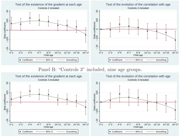
Although the primary focus of this paper is on the relationship between household income and child health, we briefly explore in this subsection the association between maternal education and child general health. Case et al. (2002) and Currie and Stabile (2003) find that in the US and Canada, maternal education is positively related to child health, and that this effect is flat over time. To investigate whether these findings also hold in the UK, we estimate equations (1) and (2) using the FACS data and represent the coefficients on maternal education as a function of child age. Our measure of maternal education is a dummy for whether the mother left school at 17 years of age or later. Our regressions either control for “controls 2” or “controls 3.” The results are presented in Figure 5.

The figures on the left hand side suggest that from birth to age 3, the education gradient is either very small (and significant) or insignificant, depending on the specification. Then, from age 4 to age 9, the gradient is positive and significant. Afterwards, for children above 10 years of age, we no longer observe any significant association between maternal education and child general health.

The figures on the right hand side imply that the effect of maternal education on child health is almost flat from birth to age 15. This result is very similar to that in the previous literature on Canada and the US. One of the two models indicate that the effect of maternal education on child health at ages 16-17 is significantly smaller than its effect at ages 0-1.

[Insert Figure 5 here]

7

Conclusion

Previous studies on the gradient in childhood in the UK have produced mixed findings regarding the effect of family income on child general health and its evolution with child age. In this paper, we undertake a comprehensive examination of the effect of family income on child general health in the UK, using the FACS. As far as we are aware, this paper is the first to use such a large dataset to shed light on the gradient in childhood in the UK. The data enables us to take a closer look at the age-profile of the gradient than the previous literature, to reduce the bias due to the endogeneity of income, and to examine the role of specific health problems in the gradient in general health.

Our findings indicate that there is no correlation between family income and child general health for infants, that the correlation becomes significant around age 2, and remains stable from 2 to 17. These results contrast with previous findings on the gradient in childhood in the UK. Furthermore, these correlations could reflect a causal impact of family income on child health. In addition, specific health problems play a role in the gradient in general health. Taken together, these results suggest that income is an important factor in explaining child health in the UK. Finally, we provide some evidence that the use of health care services, housing conditions, nutrition, and clothing are probably not important mechanisms underlying the gradient.

Our study suggests several directions for future research. A first goal could be to identify some of the mechanisms that mediate the relationship between income and child health. Second, it would be worthwhile explaining the differences in the gradient between countries. indeed, Case et al. (2002) and Currie and Stabile (2003) prove that there is a gradient that increases with child age in the US and Canada. In contrast, Reinhold and J¨urges (2011) show that the gradient does not steepen with age in Germany. Finally, our paper demonstrates that the gradient is stable across childhood years in the UK. It is an open question whether these differences in the evolution of the gradient with age are related to differences in national health care systems or other country-specific features. Finally, future research could also investigate the role of child health in the intergenerational transmission of socioeconomic status, in the UK. Indeed, this paper suggests that parental income is an important determinant of child health, and child health is associated with health capital accumulation in childhood and socioeconomic status in adulthood (Curie, 2008). It would thus be worth investigating whether child health is one of the reasons underlying the intergenerational transmission of socioeconomic status.

References

Adler, N. E., Boyce, T., Chesney, M. A., Cohen, S., Folkman, S., Kahn, R. L., Syme, S. L., 1994. Socioeconomic status and health: the challenge of the gradient. American Psychologist 49(1), 15-24.

Ai, C., Norton, E. C., 2003. Interaction terms in logit and probit models. Economics Letters 80(1), 123-129.

Allin, S., Stabile, M., 2012. Socioeconomic status and child health: what is the role of health care, health conditions, injuries and maternal health? Health Economics, Policy and Law 7(2), 227-242.

Blaxter, M., 1989. A comparison of measures of inequality in morbidity. In J. Fox (Ed.), Health Inequalities in European Countries. Aldershot: Gower.

Blaxter, M., 1990. Health and Lifestyles. London: Routledge.

Burgess, S., Propper, C., Rigg, J., 2004. The impact of low income on child health: evidence from the ALSPAC Birth Cohort Study. CMPO Working Paper Series No. 04/98.

Case, A., Lee, D., Paxson, C., 2008. The income gradient in children’s health: a comment on Currie, Shields and Wheatley Price. Journal of Health Economics 27(3), 801-807. Case, A., Lubotsky, D., Paxson, C., 2002. Economic status and health in childhood: the

origins of the gradient. American Economic Review 92(5), 1308-1344.

Condliffe, S., Link, C. R., 2008. The relationship between economics status and child health: evidence from the United States. American Economic Review 98(4), 1605-1618.

Currie, J., 2008. Healthy, wealthy and wise: socio-economic status, poor health in child-hood, and human capital development. NBER Working Paper No. 13897.

Currie, J., Lin, W., 2007. Chipping away at health: more on the relationship between income and child health. Health Affairs 26(2), 331-344.

Currie, A., Shields, M. A., Price, S. W., 2007. The child health/family income gradient: evidence from England. Journal of Health Economics 26(2), 213-232.

Currie, J., Stabile, M., 2003. Socioeconomic status and child health: why is the relation-ship stronger for older children. American Economic Review 93(5), 1813-1823. Deaton, A., Paxson, C., 1998. Aging and inequality in income and health. American

Economic Review Paper and Proceedings 88, 248253.

Deaton, A., Paxson, C., 1999. Mortality, education, income, and inequality among Amer-ican cohorts. NBER Working Paper No. W7140.

Khanam, R., Nghiem, H. S., Connelly, L. B., 2009. Child health and the income gradient: evidence from Australia. Journal of Health Economics 28, 805-817.

Kruk, K. E., 2010. Parental income and the dynamics of health inequality in early childhood. Evidence from the United Kingdom. Working paper available on the 2010 EALE conference website.

Marmot, M., Bobak, M., 2000. International comparators and poverty and health in Europe. British Medical Journal 321, 1124-1128.

Norton, E. C., Wang H., Ai, C., 2004. Computing interaction effects and standard errors in logit and probit models. Stata Journal 4(2), 154-167.

Propper, C., Rigg, J., Burgess, S., 2007. Child health: evidence on the roles of family income and maternal mental health from a UK birth cohort. Health Economics 16(11), 1245-1269.

Reinhold, S., J¨urges, H., 2012. Parental income and child health in Germany. Health Economics 21(5), 562-579.

Van Doorslaer, E., Wagstaff, A., Bleichrodt, H., Calonge, S., Gerdtham, U., Gerfin, M., Geurts, J., Gross, L., Hakkinen, U., Leu, R.E., O’Donell, O., Propper, C., Puffer, F., Rodriguez, M., Sundberg, G., Winkelhake, O., 1997. Income-related inequalities in health: some international comparisons. Journal of Health Economics 16(1), 93-112. West, P., 1997. Health inequalities in the early years: is there equalization in youth?

Social Science and Medicine 44(6), 833-58.

West, P., Sweeting, H., 2004. Evidence on equalisation in health in youth from the West of Scotland. Social Science and Medicine 59, 13-27.

Wilkinson, R., Marmot, M. (Eds.), 2003. Social determinants of health: the solid facts, 2nd ed. World Health Organization.

Winkleby, M. A., Jatulis, D. E., Frank, E., Fortmann, S. P., 1992. Socioeconomic status and health: how education, income, and occupation contribute to risk factors for cardiovascular disease. American Journal of Public Health 82, 816-820.

Figure 1: The child general health/income gradient at each age

.7

.8

.9

1

Prob. good health

0 500 1000 1500 Average income

Age 0 Age 1 Age 2 Age 3

.7

.8

.9

1

Prob. good health

0 500 1000 1500 Average income

Age 4 Age 5 Age 6 Age 7

.7

.8

.9

1

Prob. good health

0 500 1000 1500 Average income

Age 8 Age 9 Age 10 Age 11

.7

.8

.9

1

Prob. good health

0 500 1000 1500 Average income

Age 12 Age 13 Age 14 Age 15

.7

.8

.9

1

Prob. good health

0 500 1000 1500 Average income

Figure 2: The child general health/income gradient at each age (linear probability models) Panel A. “Controls 1” included.

−.05 −.025 0 .025 .05 .075 .1 Beta coefficients 0 2 4 6 8 10 12 14 16 Child age Coefficient 90% CI Smoothing Controls 1 included

Test of the existence of the gradient at each age

−.05 −.025 0 .025 .05 .075 .1 Delta coefficients 0 2 4 6 8 10 12 14 16 Child age Coefficient 90% CI Smoothing Controls 1 included

Test of the evolution of the gradient with age

Panel B. “Controls 2” included.

−.05 −.025 0 .025 .05 .075 .1 Beta coefficients 0 2 4 6 8 10 12 14 16 Child age Coefficient 90% CI Controls 2 included

Test of the existence of the gradient at each age

−.05 −.025 0 .025 .05 .075 .1 Delta coefficients 0 2 4 6 8 10 12 14 16 Child age Coefficient 90% CI Smoothing Controls 2 included

Test of the evolution of the gradient with age

Panel C. “Controls 2” included, nine age groups.

−.05 −.025 0 .025 .05 .075 .1 Beta coefficients 0−1 2−3 4−5 6−7 8−9 10−11 12−13 14−15 16−17 Child age Coefficient 90% CI Smoothing Controls 2 included

Test of the existence of the gradient for each age group

−.05 −.025 0 .025 .05 .075 .1 Delta coefficients 0−1 2−3 4−5 6−7 8−9 10−11 12−13 14−15 16−17 Child age Coefficient 90% CI Smoothing Controls 2 included

Test of the evolution of the gradient with age

Notes: “Controls 1” include the child gender, age, the presence of the mother and father in the household, the ethnicity of the respondent, and the logarithm of household size. “Controls 2” include “controls 1” plus interaction terms between the mother and father presence in the household and their education level and employment status.

Figure 3: The child general health/income gradient at each age, when there is no reverse causation (linear probability models)

Panel A: “Controls 2” included, no reverse causation.

−.05 −.025 0 .025 .05 .075 .1 Beta coefficients 0 2 4 6 8 10 12 14 16 Child age Coefficient 90% CI Smoothing

No reverse causation. Controls 2 included

Test of the existence of the gradient at each age

−.05 −.025 0 .025 .05 .075 .1 Delta coefficients 0 2 4 6 8 10 12 14 16 Child age Coefficient 90% CI Smoothing

No reverse causation. Controls 2 included

Test of the evolution of the gradient with age

Panel B: “Controls 2” included, no reverse causation, nine age groups.

−.05 −.025 0 .025 .05 .075 .1 Beta coefficients 0−1 2−3 4−5 6−7 8−9 10−11 12−13 14−15 16−17 Child age Coefficient 90% CI Smoothing

No reverse causation. Controls 2 included

Test of the existence of the gradient for each age group

−.05 −.025 0 .025 .05 .075 .1 Delta coefficients 0−1 2−3 4−5 6−7 8−9 10−11 12−13 14−15 16−17 Child age Coefficient 90% CI Smoothing

No reverse causation. Controls 2 included

Test of the evolution of the gradient with age

Notes: “Controls 2” include “controls 1” plus interaction terms between the mother and father presence in the household and their education level and employment status. 67,920 observations.

Figure 4: The child general health/income gradient at each age, when there is no reverse causation and when additional controls are included (linear probability models)

Panel A: “Controls 3” included, no reverse causation.

−.05 −.025 0 .025 .05 .075 .1 Beta coefficients 0 2 4 6 8 10 12 14 16 Child age Coefficient 90% CI Smoothing

No reverse causation. Controls 3 included

Test of the existence of the gradient at each age

−.05 −.025 0 .025 .05 .075 .1 Delta coefficients 0 2 4 6 8 10 12 14 16 Child age Coefficient 90% CI Smoothing

No reverse causation. Controls 3 included

Test of the evolution of the gradient with age

Panel B: “Controls 3” included, no reverse causation, nine age groups.

−.05 −.025 0 .025 .05 .075 .1 Delta coefficients 0−1 2−3 4−5 6−7 8−9 10−11 12−13 14−15 16−17 Child age Coefficient 90% CI Smoothing

No reverse causation. Controls 3 included

Test of the existence of the gradient for each age group

−.05 −.025 0 .025 .05 .075 .1 Delta coefficients 0−1 2−3 4−5 6−7 8−9 10−11 12−13 14−15 16−17 Child age Coefficient 90% CI Smoothing

No reverse causation. Controls 3 included

Test of the evolution of the gradient with age

Notes: “Controls 3” include “controls 2” plus the regions and the mother’s health. 67,920 observations.

Figure 5: The child general health/maternal education gradient at each age (linear prob-ability models)

Panel A: “Controls 2” included, nine age groups.

−.05 −.025 0 .025 .05 Beta coefficients 0−1 2−3 4−5 6−7 8−9 10−11 12−13 14−15 16−17 Child age Coefficient 90% CI Smoothing Controls 2 included

Test of the existence of the gradient at each age

−.05 −.025 0 .025 .05 Delta coefficients 0−1 2−3 4−5 6−7 8−9 10−11 12−13 14−15 16−17 Child age Coefficient 90% CI Smoothing Controls 2 included

Test of the evolution of the correlation with age

Panel B: “Controls 3” included, nine age groups.

−.05 −.025 0 .025 .05 Beta coefficients 0−1 2−3 4−5 6−7 8−9 10−11 12−13 14−15 16−17 Child age Coefficient 90% CI Smoothing Controls 3 included

Test of the existence of the gradient at each age

−.05 −.025 0 .025 .05 Delta coefficients 0−1 2−3 4−5 6−7 8−9 10−11 12−13 14−15 16−17 Child age Coefficient 90% CI Smoothing Controls 3 included

Table 1: Comparison of the FACS with the data used in the previous literature on the gradient in childhood in the UK

Reference This paper Currie et al. (2007) Case et al. (2008) Kruk (2010) Propper et al. (2007)

Data FACS HSE MCS ALSPAC

Nature Longitudinal Cross-sectional Cohort Cohort

born in 2000-2002 born in 1991-1992 Year 2001-2008 1997-2002 1997-2005 3 waves: Child observed at

2001-03, 2003-05, 2006 6, 18, 30 and 81 months No. observations 78,541 or less 13,745 19,567

No. children 13,745 19,567 12,000-13,000 10,000 or less

Child age 0-17 0-15 0-6 0-7

Child general health Available Available Available in wave 3 Available Assessed by parents Assessed by parents at ages 0-12 Assessed by mother

and by child at ages 13-15

Current income Exact level 32 brackets Brackets Financial hardship + income in brackets

Average income Computed Not available Computed No. of times in financial hardship since birth