Stochastic gravitational wave background : detection methods in non-Gaussian regimes

HAL Id: tel-01587686

https://tel.archives-ouvertes.fr/tel-01587686

Submitted on 14 Sep 2017

HAL is a multi-disciplinary open access

archive for the deposit and dissemination of sci-entific research documents, whether they are pub-lished or not. The documents may come from teaching and research institutions in France or abroad, or from public or private research centers.

L’archive ouverte pluridisciplinaire HAL, est destinée au dépôt et à la diffusion de documents scientifiques de niveau recherche, publiés ou non, émanant des établissements d’enseignement et de recherche français ou étrangers, des laboratoires publics ou privés.

Lionel Martellini

To cite this version:

Lionel Martellini. Stochastic gravitational wave background : detection methods in non-Gaussian regimes. Other. Université Côte d’Azur, 2017. English. �NNT : 2017AZUR4031�. �tel-01587686�

École doctorale Science Fondamentales et Appliquées

Unité de recherche UMR 6161

Thèse de doctorat

Présentée en vue de l’obtention du

grade de docteur en Astrophysique Relativiste

de

l’UNIVERSITE COTE D’AZUR

par

Lionel Martellini

Le Fond Gravitationnel Stochastique:

Méthodes de Détection en Régimes

Non-Gaussiens

Dirigée par Tania Régimbau

Soutenue le 23 Mai 2017 Devant le jury composé de :

Mme Chiara Caprini, chargée de recherche CNRS, APC Examinatrice M. Nelson Christensen, directeur de recherche CNRS, OCA Examinateur M. Jean-Daniel Fournier, directeur de recherche CNRS, OCA Examinateur Mme Tania Regimbau, chargée de recherche CNRS, OCA Directrice de thèse M. Joseph Romano, professeur, University of Texas Rio Grande Valley Rapporteur

École doctorale Science Fondamentales et Appliquées

Unité de recherche UMR 6161

Thèse de doctorat

Présentée en vue de l’obtention du

grade de docteur en Astrophysique Relativiste

de

l’UNIVERSITE COTE D’AZUR

par

Lionel Martellini

Stochastic Gravitational Wave

Background: Detection Methods in

Non-Gaussian Regimes

Dirigée par Tania Régimbau

Soutenue le 23 Mai 2017 Devant le jury composé de :

Mme Chiara Caprini, chargée de recherche CNRS, APC Examinatrice M. Nelson Christensen, directeur de recherche CNRS, OCA Examinateur M. Jean-Daniel Fournier, directeur de recherche CNRS, OCA Examinateur Mme Tania Regimbau, chargée de recherche CNRS, OCA Directrice de thèse M. Joseph Romano, professeur, University of Texas Rio Grande Valley Rapporteur

Acknowledgments 1

Résumé 2

Summary 3

Résumé Substantiel 4

1 Introduction 11

2 Gravitational Waves: Theory, Detection and Sources 17 2.1 Introduction to General Relativity, Cosmology and Gravitational Waves . 17

2.1.1 Introduction to General Relativity . . . 18

2.1.2 Application of GR to Cosmology . . . 35

2.1.3 Gravitational Waves . . . 48

2.2 Detectors of Gravitational Waves . . . 61

2.2.1 Resonant Detectors . . . 62

2.2.2 Laser Interferometers . . . 63

2.3 Sources and Types of Gravitational Waves . . . 71

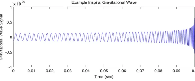
2.3.1 Inspiral GW Signals . . . 73

3 Definition and Detection of the Stochastic Gravitational Wave

Back-ground 84

3.1 Definition and Origins of Stochastic Gravitational Wave Backgrounds . . 85

3.1.1 Stochastic Gravitational Wave Background of Astrophysical Origin 85 3.1.2 Stochastic Gravitational Wave Background of Cosmological Origin 89 3.2 Standard Detection Methods for Stochastic Gravitational Wave Backgrounds 91 3.2.1 Frequentist Approach to SGWB Data Analysis . . . 92

3.2.2 Bayesian Approach to SGWB Data Analysis . . . 110

3.3 Analysis of Non-Gaussian SGWB Distributions . . . 116

3.3.1 Stylized Analysis of the Distribution of the GW Signal Given by the Superposition of a Random Number of Sources . . . 117

3.3.2 Non-Gaussian SGWB Distributions and the Edgeworth Expansion 126 4 A Semi-Parametric Approach to the Detection of Non-Gaussian Sto-chastic Gravitational Wave Backgrounds 139 4.1 Detection Methods for Non-Gaussian Gravitational Wave Backgrounds . 141 4.1.1 Gram-Charlier and Edgeworth Expansions . . . 142

4.1.2 Maximum Likelihood Estimators for the Cumulants of the SGWB Signal . . . 150

4.1.3 Implications for SGWB Signal Detection . . . 155

4.2 Numerical Illustrations . . . 162

4.2.1 Edgeworth Expansions of Usual Distributions . . . 162

4.2.2 Monte Carlo Simulations and Predictions . . . 166 4.3 Extending the Approach to the Detection of Signals in the Popcorn Regime169 5 Efficiency of the Cross-Correlation Statistic for Gravitational Wave

of Non-Gaussian Noise (and Signal) Distributions . . . 177

5.1.1 Assumptions and Notation . . . 177

5.1.2 Evidence of non-Normality in LIGO Data . . . 178

5.1.3 Distribution of the Cross-Correlation Detection Statistic . . . 179

5.1.4 Distribution of the Cross-Correlation Detection Statistic . . . 182

5.1.5 Implications for the SGWB Signal Detection with the Standard CC Statistic . . . 183

5.2 Estimation and Detection Methods for Gaussian Signal and Non-Gaussian Noise Distributions . . . 194

5.2.1 Full Gaussian Case . . . 195

5.2.2 Gaussian Signal and Non-Gaussian Noise . . . 196

5.2.3 Non-Gaussian Signal and Noise Distributions . . . 200

5.2.4 Derivation of the Optimal Cross-Correlation Statistic in the Pres-ence of Non-Gaussian Noise and SGWB Distributions . . . 204

6 Conclusions and Perspectives 213

a research collaboration with someone from a different academic field, and for making it work. Your continuous support over the last 5 years as a coauthor, as a PhD advisor, and also as a person, has truly meant a lot to me. I can only hope that we will maintain the same level and quality of interactions over the next 5 years and beyond. I also would like to thank Chiara Caprini, Nelson Christensen, Jean-Daniel Fournier, Joseph Romano and Mairi Sakellariadou for accepting to be members of my thesis committee. I feel fortunate to have such a distinguished group of astronomers and astrophysicists look over my work and provide comments and suggestions. A particularly large piece of gratitude goes to Nelson Christensen, who has offered extremely detailed feedback on a preliminary version of the document, and to Joe Romano, who has identified an inconsistency in the analysis presented in a previous version chapter 5 and has provided most helpful guidance in the revision process. Frans Pretorious and Paul Steinhardt, who have let me sit in their General Relativity and Cosmology PhD courses at Princeton University and gracefully answered my many naive questions along the way, have played an important role in my formal education in relativistic astrophysics, and for this I am grateful to them as well. On a different note, I would like to thank my father for having given me the taste for science, and my mother for having given me the taste for happiness. I finally would like to thank Daphne, Adhara, Calypso, Raphael and Theodore for their love, that mysterious form of energy that fuels every one of my steps.

fond stochastique d’ondes gravitationnelles engendré par la superposition d’un nombre élevé de signaux gravitationnels aléatoires indépendants d’origine astrophysique ou cos-mologique. La plupart des méthodes de détection du fond gravitationnel stochastique re-posent sur l’hypothèse simplificatrice selon laquelle sa distribution ainsi que celle du bruit des détecteurs sont Gaussiennes. Le sujet principal de cette thèse est la mise en place de méthodes améliorées de détection du fond gravitationnel stochastique qui tiennent compte explicitement du caractère non-Gaussien de ces distributions. En utilisant un développe-ment d’Edgeworth à l’ordre 4, nous obtenons dans un premier temps une expression analytique pour la statistique du rapport de vraisemblance en présence d’une distribu-tion non-Gaussienne du fonds gravitadistribu-tionnel stochastique. Cette expression généralise l’expression habituelle lorsque la skewness (ou coefficient de symétrie) et l’excès de kur-tosis (ou coefficient d’aplatissement) de la distribution du fond stochastique sont non nuls. Sur la base de simulations stochastiques pour différentes distributions symétriques présentant des queues plus épaisses que celles de la distribution Gaussienne, nous mon-trons par ailleurs que le 4eme cumulant peut-être estimé avec une précision acceptable lorsque le ratio signal à bruit est supérieur à 1%, ce qui devrait permettre d’apporter des contraintes supplémentaires intéressantes sur les valeurs de paramètres issus des modèles astrophysiques et cosmologiques. Dans un deuxième temps, nous cherchons à analyser l’impact sur les méthodes de détection du fond gravitationnel stochastique de dévia-tions par rapport à la normalité dans la distribution du bruit des détecteurs. Pour des valeurs raisonnables des paramètres, nous montrons que tenir compte explicitement de la non-normalité de la distribution du bruit a un impact substantiel sur les méthodes de détection, et conduit à des estimations plus élevées des probabilités de non-détection pour des niveaux donnés de probabilités de fausse alarme.

tional wave backgrounds that are expected to arise from a large number of random, independent, unresolved events of astrophysical or cosmological origin. Most detection methods for gravitational waves are based upon the assumption of Gaussian gravita-tional wave stochastic background signals and noise processes. Our main objective is to improve the methods that can be used to detect gravitational backgrounds in the presence of non-Gaussian distributions. We first maintain the assumption of Gaussian noise distributions so as to better focus on the impact of deviations from normality of the signal distribution in the context of the standard cross-correlation detection statistic. Using a 4th-order Edgeworth expansion of the unknown density for the signal and noise distributions, we first derive an explicit expression for the non-Gaussian likelihood ratio statistic, which is obtained as a function of the variance, but also skewness and kurtosis of the unknown signal and noise distributions. We use numerical procedures to gen-erate maximum likelihood estimates for the gravitational wave distribution parameters for a set of symmetric heavy-tailed distributions, and we find that the fourth cumulant can be estimated with reasonable precision when the ratio between the signal and the noise variances is larger than 1%, which should be useful for analyzing the constraints on astrophysical and cosmological models. In a second step, we analyze the efficiency of the standard cross-correlation statistic in situations that also involve non-Gaussian noise distributions. For reasonable parameter values, we find that properly accounting for the presence of non-Gaussian distributions as opposed to wrongly assuming that higher-order cumulants of the noise distributions are zero has material implications in the implemen-tation of standard detection procedures in that it generates substantially higher values for probabilities of false dismissal corresponding to given levels of probabilities of false alarm.

temps se propageant à la vitesse de la lumière, engendrées par une modification brutale et asymétrique du contenu de masse-énergie en un point de l’univers, et dont l’existence a été prédite en 1916 par Albert Einstein [73] comme conséquence de la théorie de la relativité générale qu’il avait introduite à l’occasion de 4 papiers publiés en Novembre 1915 ([72], [67], [71] and [66]). La première confirmation observationnelle de l’existence des OGs fut apportée par Hulse et Taylor en 1975 par l’observation du système bi-naire PSR1913+16 [98], et l’analyse de la perte d’énergie de ce système par Taylor et Weisberg en 1982 [164] (voir également [165], [177], et [176] pour des analyses plus ré-centes du système PSR1913+16). Ces travaux ont montré que la période orbitale du système binaire PSR1913+16 constitué de deux étoiles à neutrons décroissait d’un mil-lième de seconde par an, une mesure en accord avec la prévision théorique concernant l’émission d’ondes gravitationnelles pour un tel système. A la suite de cette détection indirecte, la détection directe d’un signal d’OG est devenue une question centrale en astrophysique relativiste, et d’importantes ressources ont été consacrées à la mise au point d’interféromètres permettant de détecter ces OGs. Le 14 Septembre 2015, la nou-velle génération des détecteurs LIGO, situés respectivement à Hanford dans l’Etat de Washington et à Livingston dans l’Etat de Louisiane, a permis de détecter un signal gravitationnel [9]. L’analyse de l’amplitude des ondes et de l’évolution de leur fréquence a révélé qu’elles avaient été produites par la coalescence d’un système binaire composé de deux trous noirs situés à environ 410 Megaparsec de notre galaxie, respectivement de 29 et de 36 fois la masse du Soleil. Cette fusion a engendré un trou noir de 62 fois la masse du Soleil, les 3 masses solaires manquantes ayant été dissipées sous forme d’ondes gravitationnelles. Une deuxième détection a eu lieu le 26 Décembre 2015, qui a porté à nouveau sur la coalescence d’un système binaire composé de deux trous noirs situés à en-viron 440 Megaparsec de notre galaxie, respectivement de 14.2 et de 7.5 masses solaires. Ces récentes détections, qui suggèrent que la population des binaires de trous noirs est

de l’astronomie gravitationnelle, et l’on s’attend désormais à ce qu’une troisième généra-tion de détecteurs (projets Einstein Telescope [142], LIGO Voyager ou Cosmic Explorer [124]) permette d’augmenter la probabilité de détecter des OGs de magnitude encore plus faible grâce à des gains de sensibilité supplémentaires.

Au-delà des signaux gravitationnels individuels résolus comme GW150914 et GW151226, les interféromètres de nouvelle génération devraient nous permettre de détecter le fond stochastique d’OGs engendré par l’addition d’un nombre élevé de signaux gravitationnels aléatoires indépendants non résolus d’origine astrophysique ou cosmologique. La stratégie optimale de détection du fond gravitationnel stochastique consiste à prendre le produit croisé des détections d’au moins deux détecteurs afin d’éliminer au mieux le bruit de l’instrument [15]. Dans le cadre d’hypothèses classiques incluant la présence de distribu-tions stationnaires et de corrélation temporelle nulle pour les signaux stochastiques et le bruit, ainsi que la présence de détecteurs de même sensibilité, il est possible de montrer que cette statistique de détection dite de cross-correlation (CC) est optimale au sens où elle permet de minimiser la probabilité de rejeter à tort l’hypothèse d’une détection pour un taux donné de fausse alarme (voir par exemple [44, 78, 15]). Les méthodes standard de détection des OGs reposent par ailleurs sur l’hypothèse simplificatrice selon laquelle le fond gravitationnel stochastique est distribué de façon Gaussienne. Des travaux récents portant sur une modélisation réaliste de la population des objets astrophysiques de na-ture à engendrer des OGs d’amplitude assez forte pour être détectées laisse cependant supposer qu’il n’existe pas un nombre de sources superposées assez élevé pour permettre l’application du théorème central limite, et que le fond stochastique résultant de la su-perposition de ces signaux aléatoire peut donc faire apparaître des déviations par rapport à l’hypothèse de normalité. Il a également été montré que le fond stochastique engendré par des cordes cosmiques pourrait être dominé par la contribution non-Gaussienne des sources les plus proches [55, 144].

de sa distribution, ce qui devrait permettre d’améliorer l’efficacité de la procédure de détection, et également de potentiellement permettre de distinguer le fond d’origine as-trophysique du fond d’origine cosmologique. L’approche que nous proposons dans un premier temps est basée sur le développement d’Edgeworth, qui est un développement formel en série infinie permettant d’écrire la fonction caractéristique d’une distribution non-Gaussienne inconnue comme une perturbation autour de la fonction caractéristique de la distribution Gaussienne. Dans la mesure où le développement d’Edgeworth a pré-cisément vocation à caractériser la déviation à la normalité dans le cadre d’une application à distance finie du théorème central limite, il apparaît naturellement adapté à l’analyse du fond gravitationnel stochastique résultant de la superposition d’un nombre fini de sources d’origine astrophysique, sous réserve que la non-Gaussianité ainsi engendrée ne soit pas trop forte. En utilisant un développement d’Edgeworth poussé jusqu’à l’ordre 4, nous avons réussi à obtenir une expression analytique pour la statistique de détection dans un cadre non-Gaussien qui fait intervenir non seulement la variance mais aussi le coefficient d’asymétrie (skewness) et le coefficient d’aplatissement (kurtosis) de la distribution du signal. Cette expression généralise l’expression habituelle, qui est obtenue comme cas particulier de l’expression générale lorsque les cumulants d’ordre 3 et 4 de la distribution du fond stochastique sont nuls, comme c’est le cas pour une distribution Gaussienne. Sur la base de simulations stochastiques pour différentes distributions symétriques présen-tant des queues plus épaisses que celles de la distribution Gaussienne, nous montrons par ailleurs que le 4eme cumulant peut-être estimé avec une précision acceptable lorsque le ratio signal à bruit est supérieur à 1%. Cette valeur de 1% est à comparer à la valeur attendue du rapport signal à bruit pour la détection du fond gravitationnel stochastique par la deuxième génération des détecteurs LIGO et Virgo (Advanced LIGO et Advanced Virgo) et par Einstein Telescope, valeur qui est comprise entre 1% et 10%. Pour les cordes cosmiques, la valeur de la densité d’energie à une fréquence de 100 Hz est attendue entre

Telescope. Pour les fusions d’objets compacts, la valeur de la densité d’energie à une fréquence de 100 Hz est attendue entre les valeurs 10−10 _{et 10}−7_{, ce qui correspond à un} rapport signal à bruit de 10−7 _{à 0.01 pour la deuxième génération des détecteurs LIGO} et Virgo et de 10−5 _{à 1 pour Einstein Telescope.}

L’intérêt principal de la méthode est précisément de permettre l’estimation de paramètres supplémentaires, à savoir les cumulants d’ordre 3 et 4 de la distribution du signal grav-itationnel, ce qui devrait permettre d’apporter des contraintes supplémentaires intéres-santes sur les valeurs de paramètres issus des modèles astrophysiques et cosmologiques. Il s’avère par exemple impossible de distinguer, dans le cadre des méthodes d’estimation traditionnelles de type cross-correlation (CC), un fond stochastique provenant de sys-tèmes de binaires compactes (étoiles à neutron et/ou trous noirs) caractérisés par un taux de coalescence élevé et des masses faibles, ou bien un taux de coalescence faible et des masses élevées car ces deux situations peuvent donner un signal de même amplitude [126]. La méthode introduite ici pourra en principe permettre de distinguer ces deux situations très différentes sur le plan astrophysique par l’estimation du cumulant d’ordre 4, sachant que le premier cas (taux élevé et masses faibles) correspond à un signal de type continu et une valeur faible de la kurtosis tandis que le deuxième cas (taux faible et masses élevées) correspond au contraire a un signal de type "popcorn" avec une valeur élevée de la kurtosis. Au final, l’un des avantages principaux de l’approche proposée est son caractère non-paramétrique, qui permet de s’affranchir de la nécessite de faire des hypothèses restrictives à propos de la nature exacte de la distribution non-Gaussienne sous-jacente. Les méthodes développées dans le cadre de ces travaux pourraient a priori être utilisées dans le cadre d’un effort de distinction du fond d’origine astrophysique et du fond d’origine cosmologique, sous réserve que les déviations à la normalité admettent dans ces deux cas des signatures bien distinctes.

raisons de penser que le bruit instrumental ou environnemental est également distribué de manière non-Gaussienne [181], et il est alors utile de chercher à analyser l’impact sur les méthodes de détection du fond gravitationnel stochastique de ces déviations par rapport à la normalité dans la distribution du bruit. Par ailleurs, l’hypothèse standard selon laquelle les détecteurs auraient la même sensibilité pourrait ne pas être strictement vérifiée lors des étapes intermédiaires de calibration des détecteurs de deuxième génération Advanced LIGO and Advanced Virgo, et une telle hypothèse serait encore plus discutable dans le cas d’observations jointes impliquant des détecteurs de deuxième et troisième générations. Dans ce contexte, nous cherchons à analyser la performance de la statistique CC standard dans des situations impliquant des déviations des hypothèses évoquées ci-dessus, et en particulier des situations impliquant la présence de non-normalité dans la distribution du bruit des détecteurs.

Pour cela, nous montrons d’abord qu’il est possible d’obtenir une expression général-isée pour la statistique du rapport de vraisemblance dans un cadre de travail impliquant une déviation de la normalité non seulement pour le signal mais aussi pour le bruit des détecteurs. Cette expression analytique permet d’envisager une estimation efficace des paramètres de variance, skewness et kurtosis de la distribution du signal et du bruit des détecteurs. En parallèle a l’identification des estimateurs du maximum de vraisemblance, nous introduisons également des estimateurs basés sur la méthode dite des moments, qui sont sans biais par construction. Pour des valeurs raisonnables des paramètres, nous montrons que tenir compte explicitement de la non-normalité de la distribution du bruit a un impact substantiel sur les méthodes de détection. Nous introduisons en particulier une expression analytique pour l’espérance et la variance de la statistique de détection standard dans un cadre non-Gaussien, et nous montrons pour des valeurs raisonnables des paramètres que tenir compte explicitement de la non-normalité de la distribution du bruit a un impact substantiel sur les méthodes de détection, et conduit à des estimations

résultats suggèrent également qu’il est possible d’obtenir une statistique de détection op-timale dans un cadre non-Gaussien généralisé. Cette statistique de détection généralise la statistique de détection standard, qui est recouverte pour des valeurs nulles des cumulants d’ordre 3 et 4 des distributions du signal et du bruit.

Introduction

Gravitational waves (GWs in short) are perturbations of spacetime geometry travelling at the speed of light created by asymmetric acceleration of masses or non stationary fields, which existence is predicted by the theory of general relativity (GR in short). While elec-tromagnetic waves interact strongly with matter, GWs minimally interacting with the matter they encounter, which allows us to probe astrophysical or cosmological phenom-ena that cannot be observed by electromagnetic signals, such as the inspiral, coalescence and merger of black holes, the collapse of a stellar core, or the dynamics of the early Universe. The first observational validation of the existence of gravitational waves is the PSR B1913+16 binary pulsar system discovered by Hulse and Taylor in 1975 [98], and for which Taylor and Weisberg [164] subsequently demonstrated that the rate of decay of the orbit exactly matches GR predictions regarding the loss of energy of the system due to the emission of gravitational waves (see also [165], [177], and [176] for more recent observations and related analyses). Following this first indirect evidence of the existence of GWs, the direct detection of GWs has become a question of central importance in relativistic astrophysics, and an increasing range of efforts has been dedicated to the design of improved detectors. On September 14, 2015, second generation Laser Interfer-ometer Gravitational-Wave Observatory detectors (known as Advanced LIGO detectors),

located in Hanford, Washington, and Livingston, Louisiana, USA, have successfully de-tected GWs produced during the late inspiral and merger of two black holes of masses respectively 29 and 36 solar masses, located at approximately 410 Megaparsec from our galaxy [9]. The black hole resulting from the merger had a total mass of 62 solar masses, with the missing 3 solar masses having been carried away under the form of gravitational waves. A second detection of gravitational waves generated by the coalescence of a bi-nary system of stellar mass black holes subsequently took place on December 26, 2015 [5]. These remarkable detections have opened a new era of astronomy, and third-generation interferometers such as Einstein Telescope [142], LIGO Voyager or Cosmic Explorer [124] are expected to further increase the likelihood of detecting the exceedingly small effects of gravitational waves.

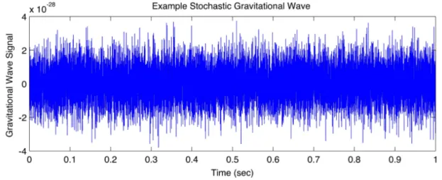
In addition to resolved individual GW signals such as GW150914 and GW151226, the new generations of interferometers should allow us to detect stochastic GW backgrounds, which are expected to arise from a large number of random, independent, unresolved events of astrophysical or cosmological origin. The optimal detection strategy to search for a stochastic background is to cross correlate the output of two detectors (or of a network of detectors) to eliminate the instrumental noise [15]. Under standard assumptions including stationary and serially uncorrelated Gaussian gravitational wave stochastic background signal and noise processes as well as homogenous detector sensitivities, the standard cross-correlation (CC in short) detection statistic is known to be optimal in the sense of minimizing the probability of a false dismissal at a fixed value of the probability of a false alarm (see for example [44, 78, 15]). While the GW background is usually assumed to be Gaussian invoking the central limit theorem, and thus completely characterized by its mean and variance, recent predictions based on population modeling suggest that for many astrophysical models, there may not be enough overlapping sources, resulting in the formation of a non-Gaussian background. [182] show that the population of binary black hole systems in the observable universe could produce for reasonable mass and rate parameter values a series of non-continuous background burst signals that will most likely

be of the shot noise or at most popcorn noise type (see section 3.1 for precise definitions) in the Advanced LIGO/Virgo frequency range, while the signal will be continuous but not necessarily Gaussian for ET type-detectors depending upon assumed parameter values. Turning to cosmological sources of gravitational waves, it has also been shown that the background from cosmic strings could be strongly non-Gaussian [55, 144] (see section 3.1.2 for more details).

Our work has a main focus on improving the methods that can be used to detect non-Gaussian GW backgrounds, which would permit to possibly distinguish between as-trophysical and cosmological GW backgrounds and gain confidence in a detection. The approach we propose in a first step is based on Edgeworth expansion, which is a formal asymptotic expansion of the characteristic function of the signal distribution, whose un-known probability density function is to be approximated in terms of the characteristic function of the Gaussian distribution. Since the Edgeworth expansion provides asymp-totic correction terms to the Central Limit Theorem up to an order that depends on the number of moments available, it is ideally suited for the analysis of stochastic gravita-tional wave backgrounds generated by a finite number of astrophysical sources. It is also well-suited for the analysis of signals from cosmological origin in case the deviations from the Gaussian assumption are not too strong. Using a 4th-order Edgeworth expansion, we obtain an explicit expression for the nearly optimal non-Gaussian likelihood statistic that is obtained as a function of the variance, but also skewness and kurtosis, of the unknown signal distribution. This expression generalizes the standard maximum likelihood detec-tion statistic, which is recovered in the limit of vanishing third and fourth cumulants of the empirical conditional distribution of the detector measurement. We use numerical procedures to generate maximum likelihood estimates for the gravitational wave distrib-ution parameters for a set of symmetric heavy-tailed distribdistrib-utions, and we find that the fourth cumulant can be estimated with reasonable precision when the ratio between the signal and the noise variances is larger than 1%. The main benefit of the procedure is precisely that it allows us to estimate additional parameters, namely the 3rd and 4th

cumulants of the gravitational wave signal distribution, which should be useful for ana-lyzing the constraints on astrophysical and cosmological models that will be imposed by observed gravitational wave signals, and comparing them to the constraints derived from supernovae or galaxy clusters observations. Overall, one key advantage of the proposed methodology, which relies on an explicit correction to the central limit theorem when the number of sources is finite, is that can be applied without any assumption regarding the exact nature of the departure from normality.

In this first step, we maintain the assumption of Gaussian noise distributions so as to better focus on the impact of deviations from normality of the signal distribution in the context of the standard cross-correlation detection statistic. This assumption is at odds, however, with accumulated evidence of strong deviations from the Gaussian assumption for noise distributions in gravitational waves detectors [125]. A recent paper [181] intro-duces a new measure for characterizing the non-Gaussian noise component modelled as a Student-t distribution and reveals stationary and transient deviations from Gaussianity in LIGO S5 data. This is a serious concern since existing detection strategies for both deterministic and stochastic signals are expected to deteriorate when non-Gaussian noise is present [13, 14]. If the exact non-Gaussian nature of the detector noise is understood, it is possible to introduce a robust detection statistic using the specific non-Gaussian noise assumption (see for example [16] for a detection method based on an exponentially distributed noise process, and [152] for a detection method based on a Student’s t dis-tributed noise process). Given that the actual noise distribution is a priori unknown, it is unclear how much improvement, if any, these methods would allow with respect to the standard method based upon a Gaussian assumption in case of a misspecification of the exact deviation from the Gaussian assumption. In this context, we analyze the efficiency of the CC statistic in situations that deviate from the Gaussian assumption for both the stochastic gravitational wave signal distribution and detector noise distributions. To do so we first show how to obtain consistent estimates for the first four cumulants of the signal and noise distributions using a suitable extension of the likelihood function, for

which we derive an analytical expression. These results extend our previous results where we have Focused on a situation involving a non-Gaussian signal distribution, but have maintained the assumption of a Gaussian noise distribution. In addition to obtaining parameter estimates through maximum likelihood techniques, we also introduce so-called moment-based estimators given by analytical functions of the joint observations from the two detectors. While the moment-based estimators for the variance of the signal and the noise in each detector coincide with the maximum likelihood estimators in the Gaussian case, the moment-based estimators may be different in a generalized non-Gaussian setting but they share with maximum likelihood estimators the desirable property to be unbiased by construction. Turning to a numerical analysis, we find that properly accounting for the presence of non-Gaussian distributions as opposed to wrongly assuming that higher-order cumulants of the noise distributions are zero has material implications in the implemen-tation of standard detection procedures in that it generates higher values for probabilities of false dismissal corresponding to given levels of probabilities of false alarm. The correc-tion is found to be particularly substantial when detector sensitivities exhibit substantial differences, a situation that is expected to hold in early phases of development of the Advanced LIGO-Virgo detectors before they reach their design sensitivity. Under such circumstances, or in joint detections from Advanced LIGO and the Einstein Telescope project [142], failing to account for the presence of non-Gaussian detector noise distribu-tions In addition to their implicadistribu-tions for the performance of the standard CC detection statistic, we also discuss the implications of our results for the derivation of an optimal detection statistic in a non-Gaussian context.

The rest of this thesis is organized as follows. In chapter 2, we provide a broad introduction to the theory of general relativity and its implications for the generation of gravitational waves. In chapter 3, we propose an analysis of the stochastic gravitational wave background and its distribution. In chapter 4, we introduce a semi-parametric approach to the detection of non-Gaussian stochastic gravitational wave backgrounds. In chapter 5, we analyze the efficiency of the standard cross-correlation statistic in the

presence of non-Gaussian detector noise distributions and discuss the implications for the derivation of an optimal detection statistic in a non-Gaussian setting. Finally, we present in chapter 6 our conclusions and suggestions for further research. Note that we have chosen to write the chapters so that they can be read somewhat independently, even if this necessarily implies some redundancies.

Gravitational Waves: Theory,

Detec-tion and Sources

We first provide a brief introduction to general relativity and gravitational waves, before presenting an overview of gravitational wave detectors as well as an overview of the main sources of gravitational waves.

2.1

Introduction to General Relativity, Cosmology

and Gravitational Waves

General relativity (or GR in short) is a theory of gravitation introduced by Albert Einstein in 4 papers published in November 1915 ([72], [67], [71] and [66]). It has become the commonly accepted description of gravitation in modern physics, which provides a unified description of gravity as a geometric property of spacetime.

2.1.1

Introduction to General Relativity

The presentation that follows is broadly inspired by [39]. In what follows we adopt the usual notational convention for indices, namely greek letters α, β, γ... are used for 4-dimensional spacetime indices ranging from 0 (the time coordinate) to 3 (for the three space dimensions), while roman letters i, j, k, ... are used for 3-dimensional spatial in-dices. Throughout the text, we also use the Einstein summation convention regarding the repeated adjacent indices in upwards and downwards location. In other words, we take: uα_v α ≡ 3 α=0 uα_v α. (2.1)

The Special Theory of Relativity (SR): Principle of Relativity and Spacetime Geometry with Inertial Reference Frames

The special theory of relativity published in the "annus mirabilis" 1905 ([70], [69]) by Albert Einstein is based upon the assumption that there is no preferred inertial reference frame, or in other words that measurements of physical quantities and expressions of physical laws remain the same after changing from a reference frame to another reference frame that is in constant rectilinear motion with respect to the original one. In particular, this postulate implies that the speed of light will yield the same measure c = 299, 792, 458 ms−1 _{in all referential frames. The geometric structure of the spacetime used in special} relativity is the so-called Minkowski (or Poincaré-Minkowski) spacetime, a generalization of the Euclidean space where the squared distance ds2 _{between the point P = (x1, x2, x3)} (we sometimes also use the notation x, y, z for the 3 spatial coordinates) and an infini-tesimally close point Q = (x1+ dx1, x2+ dx2, x3+ dx3) is given by Pythagorean theorem as:

Minkowski spacetime is a flat spacetime where physical events are described in terms of spacetime coordinates (t, x1, x2, x3) and where the infinitesimal spacetime interval be-tween nearby events is measured in terms of the line element ds2 _{given in Cartesian} coordinates by the following generalization of Pythagorean theorem:

ds2 =−c2_dt2_{+ dx}2

1+ dx22 + dx23, (2.3)

or equivalently by:

ds2 =_−dx2₀+ dx₁2+ dx2₂+ dx2₃, (2.4) in the coordinate system (x0 = ct, x1, x2, x3). Defining the Minkowski metric η_αβ by:

η₀₀ = −1 (2.5)

η_ii = 1 for i = 1, 2, 3 (2.6)

η_αβ = 0 for α = β, (2.7)

we can write the line element ds2 _{in Minkowski spacetime as:}

ds2 = ηαβdxαdxβ. (2.8)

In matrix notation, the metric is simply:

η =          −1 0 0 0 0 1 0 0 0 0 1 0 0 0 0 1          . (2.9)

Equation 2.8 defines the geometry of Minkowski spacetime. The symmetry group of this geometry is the group of coordinate transformations Λµ

ν : (x0, x1, x2, x3)→ (x′0, x′1, x′2, x′3) that leaves the quadratic form 2.8 of the interval ds2 _{invariant. This group of}

coordi-nate transformations, known as the Lorentz group, is therefore defined by the following transformations:

x′µ= Λµνxν + aµ, (2.10) where the so-called Lorentz boost transformation Λµ

ν satisfies the condition:

η_αβ = Λα_µΛβ_νη_µν (2.11)

so as to ensure the invariance of the line element 2.8. More generally, the principle of relativity, which requires that the laws of physics have the same expression in all inertial reference frames, implies that physical theories should be invariant under a class of transformations known as Poincaré transformations, which includes Lorentz boost transformations, but also translations and rotations. Physically, consider an observer in an initial frame of reference frame with coordinates (t, x1, x2, x3) and an observer in a different frame of reference with coordinates (t′_{, x}′

1, x′2, x′3) moving with constant velocity v along the x1-axis. The change in coordinates that leaves the spacetime interval invariant ds′ _{= ds is given by the following Lorentz-boost transformation along the x1-axis:}

                 t′ _{= γ t−} v c2x1 x′ 1 = γ (x1− vt) x′ 2 = x2 x′ 3 = x3 (2.12)

where the so-called Lorentz factor is given by:

γ ≡ 1 1₋ v2

c2

Note that for a particle with fixed space coordinates (dx2

1 = dx22 = dx23 = 0) the interval of time 2.8 elapsed as time moves forward (dt > 0) is negative:

ds2 =_−c2dt2 < 0. (2.14)

This leads us to the introduction of the proper time τ via dτ2 = dt2 =₋ds 2 c2 , (2.15) or equivalently: dτ = 1 c √ −ds2_{. (2.16)}

Proper time elapsed along a trajectory through spacetime parametrized a a function of some parameter xα_{(λ) is thus defined as the time measured by a clock following that} line, in the reference frame where the spatial coordinates do not vary (an observer on a different frame of reference will measure a different time). Integrating 2.16, we obtain that the proper time interval between two events on a trajectory is:

∆τ = 1 c √ −ds2 ₌ 1 c −ηαβdx α_dxβ _(2.17)

If the trajectory through spacetime is parametrized a a function of some parameter xα_(λ), then the proper time can be expressed as:

∆τ = 1 c −ηαβ dxα dλ dxβ dλ dλ (2.18)

We thus have from 2.17: τ = dt2₋ 1 c2 (dx 2 1+ dx22+ dx23) (2.19) = 1− 1 c2 dx1 dt 2 + dx2 dt 2 + dx3 dt 2 dt (2.20) = 1− v2(t) c2 dt = dt γ (t) (2.21)

where we have introduced the following quantity:

γ (t)≡ 1 1₋ v2_c(t)2

, (2.22)

which generalizes the Lorentz factor 2.13 to the case of a possibly time-varying velocity. The corresponding tangent vector

Uµ= dx µ

dτ (2.23)

is called the four-velocity and is is automatically normalized:

η_µνUµUν =_−1. (2.24)

A related quantity is the momentum four-vector defined by:

pµ_{= mU}µ_{, (2.25)}

where m is the rest mass of the particle. We can also define the proper distance as the distance between the two events as measured in an inertial frame of reference in which the events are simultaneous. In the same spirit, the proper length or rest length L0 of an object is the length of the object measured by an observer which is at rest relative to it, by applying standard measuring rods on the object. The measurement of the object endpoints does not have to be simultaneous, since the endpoints are constantly at rest

at the same positions in the object rest frame, so it is independent of ∆t. However, in relatively moving frames the object endpoints have to be measured simultaneously, since they are constantly changing their position.1

The General Theory of Relativity (GR): Principles of Equivalence and General Covariance and Spacetime Geometry with Accelerated Reference Frames The principle of relativity, which is the founding principle of special relativity, has been extended by Einstein to the principle of general covariance, which requires the invariance of the form of physical laws under changes of reference frames that extend beyond the inertial reference frames, and which can include accelerated reference frames. The starting point was the recognition in 1907 [68] by Albert Einstein that the equivalence between inertial mass and gravitational mass, which implies the universality of free fall (initially noted by Galilée in 1638 century, and subsequently confirmed by Newton in 1687 and von Eötvös at the end of the 19th century), can be translated as what is now known as the weak form of the equivalence principle. Based on free-fall thought experiments, this principle states the equivalence between gravitation and acceleration: gravity can be canceled (free fall) or mimicked (constant acceleration) by acceleration.

Such general accelerated reference frames are mathematically represented by arbitrary differentiable coordinate transformations. The transformation from an inertial reference frame (x0, x1, x2, x3) to a general non inertial reference frame (x′

0, x′1, x′2, x′3) is a non-linear transformation defined through the 4 functions x′α_(xµ_{) expressing the new primed} coordinates in terms of the original unprimed coordinates assumed to be expressed in an inertial frame of reference, or equivalently through the reverse transformation xµ_(x′α₎ expressing the original unprimed coordinates as functions of the new primed coordinates. The non-linearity of the transformation implies that the line element ds2 _{will take a more} complicated form in the accelerated frame of reference compared to the form given in

1_{For this reason, the distance defined in equation 2.166 is not a proper distance. Indeed, it is measured}

between two free-moving test particles subject to gravitational wave oscillations A and B as c

2(t2− t1),

where t1 is the proper time for an observer located on a reference frame attached to A who sends a light

equation 2.8 in the inertial frame of reference. Under this general transformation, and given that

dxµ= ∂x µ

∂x′αdx′α, (2.26)

starting with the line element given by special relativity in the inertial reference frame (x0, x1, x2, x3)

ds2 = η_αβdxαdxβ, (2.27) we obtain in the accelerated reference frame (x′

0, x′1, x′2, x′3): ds2 = gαβdx′αdx′β, (2.28) with gαβ = η_µν ∂x µ ∂x′α ∂xν ∂x′β.

Given the non-linearity of the 4 functions x′α_(xµ_{) , the functions gαβ exhibit in general an} explicit dependence on the coordinates xµ_{. As a result, the local geometry of spacetime} is no longer given by the simple Minkowski metric in equation 2.8 with constant coeffi-cients, but by the much more general quadratic metric in equation 2.28.2 _{In this general} spacetime endowed with the metric gµν, the invariance of the line element implies

ds2 = gµνdxµdxν = gµν∂x µ ∂x′α ∂xν ∂x′βdx ′α_dx′β _{= g}′ αβdx′αdx′β, (2.29) with: g_αβ′ = gµν ∂xµ ∂x′α ∂xν ∂x′β. (2.30)

Such general metric spaces have been introduced by the mathematicians Gauss and Riemann in the 19th century in the situation where the quadratic form is positive defi-nite.3 _{More formally, let M be a n−dimensional C}∞ _{manifold, TxM the tangent space at}

2_{The geometry is still flat, and the departure from the Minkowski merely reflects a change of}

coordi-nates.

x∈ M and T M ≡ ∪x∈MTxM the tangent bundle of M . Hence, each element of T M has the form (x, y), where x ∈ M and y ∈ TxM . In Riemannian geometry, the useful infor-mation about the curvature of a manifold is contained in the metric. We first introduce a function F , known as metric function or generator function, which measures the distance between two points x = (x1_{, x}2_{, ..., x}n_{) and x + dx = F (x}1_{+ dx}1_{, x}2_{+ dx}2_{, ..., x}n_{+ dx}n_{) :} ds = F x1, x2, ..., xn, dx1, dx2, ..., dxn . (2.31)

Here (x1_{, x}2_{, ..., x}n_{) are the coordinates assigned in a given coordinate system to point} x of M, and (dx1_{, dx}2_{, ..., dx}n_{) or (y}1_{, y}2_{, ..., y}n_{) are coordinates of y ∈ TxM , defined} through the natural basis ei = _∂x∂i _x, with y = yiei. Natural conditions (which may not

be necessary for some/all physical applications) that should be satisfied by the function F (x1_{, ..., x}n_{, y}1_{, ..., y}n_{), denoted by F (x, y), are as follows.}

1. Positivity: F (x, y) > 0 for any y = dx.

2. Positive homogeneity: F (x, py) = pF (x, y) for any p > 0 (F is a homogenous function of degree 1).4

3. Symmetry: F (x, −y) = F (x, y). (we may envision relaxing this condition, espe-cially with respect to the time dimension, so as to have a geometric representation of the time arrow)

4. Strong convexity: the Hessian matrix ∂2

∂yµ_∂yν 1₂F2 is positive-definite at every point

of the tangent bundle T M except at the origin (T M\0).

Intuitively, the value of F (x, y) is interpreted as the length of the vector y tangent at x. More formally, the function F can be used to define the length of a curve indexed by time: s = t=b t=a F (x (t) , y (t)) dt where y (t) = dx dt (t) . (2.32) as a pseudo-Riemannian metric.

If the curve is parametrized in terms of another parameter τ = τ (t), for c = τ (a) ≤ τ ≤ d = τ (b), then the length is given as:

s = τ =b τ =a

F (x (τ ) , y (τ )) dτ where y (τ ) = dx

dτ (τ ) . (2.33) Note that the length integral is independent of the parametrization if and only if condition 2 is valid. Indeed, we have then:

s = F x,dx dt dt = F x, dx dτ dτ dt dt = F x, dx dτ dτ dtdt = F x, dx dτ dτ . (2.34) We now derive a fundamental proposition that satisfies the metric function.

Proposition 1 The following relationship holds between the squared value of the metric function and the Hessian of the metric function:

F2(x, y) = 1 2y

µ_yν∂2F2(x, y)

∂yµ_∂yν (2.35)

Proof. By differentiating with respect to p the relation

pF x1, ..., xµ, ..., xn, y1, ..., yµ, ..., yn = F x1, ..., xµ, ..., xn, y1, ..., pyµ, ..., yn we obtain: F (x, y) = ∂F (x 1_{, ..., x}µ_{, ..., x}n_{, y}1_{, ..., py}µ_{, ..., y}n₎ ∂p = ∂F (x 1_{, ..., x}µ_{, ..., x}n_{, y}1_{, ..., py}µ_{, ..., y}n₎ ∂yµ ∂ (pyµ₎ ∂p = ∂F (x, y) ∂yµ y µ _(2.36)

which is Euler theorem for homogeneous functions of degree 1. By differentiating the relation p2_{F (x, y) = F (x}1_{, ..., x}µ_{, ...x}ν_{, ..., x}n_{, y}1_{, ..., py}µ_{, .., py}ν_{, ..., y}n_{) twice with respect} to p, we also obtain:

∂2_{F (x, y)}

Now, taking the derivative of the squared metric function with respect to yµ_{, we have} that: ∂F2_{(x, y)} ∂yµ = 2F (x, y) ∂F (x, y) ∂yµ Differentiating again with respect to yν_:

∂2_F2_{(x, y)} ∂yµ_∂yν = 2 ∂F (x, y) ∂yν ∂F (x, y) ∂yµ + 2F (x, y) ∂2_{F (x, y)} ∂yµ_∂yν =0from equation 2.37 = 2F2(x, y) 1 yµ_yν from equation 2.36

This result allows us to define the following covariant tensor of order 2 fµν(x, y) = 1

2y

µ_yν _× ∂2_{F (x,y)}

∂yµ_∂yν , which will be used to calculate norms of vectors and distances on the

manifold M. Indeed, we have ds ≡ F (x, y) = fµν(x, y) yµ_yν_{. As explained above,} we use in general relativity the framework of standard Riemannian geometries, where the metric tensor only depends on coordinates on the spacetime manifold and not on coordinates on the tangent space. In other words, the metric only depends on the position but not on the velocity vector and we write ds = gµν(x) yµ_yν_{. The general case} where ds ≡ F (x, y) = fµν(x, y) yµ_yν _{defines a broader class of geometries, known as} Finslerian geometries, named after Paul Finsler, a German and Swiss mathematician who received a PhD in 1918 at the University of Göttingen under the supervision of Constantin Carathéodory, with a focus on extending Riemannian geometry to more general metric specifications [12].

Connections and Covariant Differentiation

Intuitively, the difficulty in performing differential and integral calculus on a curved manifold M is that the tangent vector to a curve on the manifold does not belong to the manifold M itself, but belongs instead to its tangent bundle T M. From this arises the need to formally define how to transport a vector along a curve in a parallel and

consistent manner. An affine connection is introduced for transporting tangent vectors to a manifold from one point to another along a curve. An affine connection is typically given in the form of a covariant derivative, which defines how to operate the infinitesimal transport of a vector field in a given direction. More formally, let us consider the impact of a change of coordinates xµ_{→ x}′µ _{on a scalar field φ. From the conventional chain rule,} we have: ∂φ ∂xµ −→ ∂φ ∂x′µ = ∂xµ ∂x′µ ∂φ ∂xµ, (2.38) or equivalently: ∂µφ−→ ∂′ µφ = ∂xµ ∂x′µ∂µφ, (2.39)

where we have used the shorthand notation ∂µφ = ∂φ

∂xµ for the partial derivative of φ with

respect to xµ _{and ∂}′

µφ = ∂x∂φ′µ for the partial derivative of φ with respect to x′µ. If we now

apply the change of coordinate xµ_{→ x}′µ _{to a vector field V}ν_{, we obtain:} ∂µVν _{−→ ∂µ}′Vν′ = ∂x µ ∂x′µ∂µ ∂x′ν ∂xνV ν _(2.40) = ∂x µ ∂x′µ ∂x′ν ∂xν ∂µV ν₊ ∂xµ ∂x′µ ∂2_x′ν ∂xµ_∂xνV µ_, non-tensorial terms (2.41)

We would like to define a new form of derivative operator ∇µ, known as the covariant derivative operator, which would obey the tensorial transformation law:

∇µVν _{−→ ∇µ} ′V′ν = ∂xµ ∂x′µ ∂xν ∂x′ν∇µV ν_{. (2.42)}

To do so, we introduce the so-called Christoffel symbols Γν

µλ, or connection coefficients, which are required ingredients in the definition of the covariant derivative as the usual partial derivative plus a linear correction:

∇µVν _{= ∂}

So when given a particular metric gµν, the first step consists of calculating the connection coefficients so that we can take covariant derivatives. It can be shown that to cancel out the non tensorial terms defined in equation (2.41), the connection coefficients Γν

µλ need to obey the following transformation law under a coordinate transformation xµ _{→ x}′µ (from which we see that these connection coefficients Γν

µλ are not tensors):

Γν_µ′′_λ′ = ∂xµ ∂x′µ ∂xλ ∂x′λ ∂x′ν ∂xνΓ ν µλ− ∂xµ ∂x′µ ∂xλ ∂x′λ ∂2_x′ν ∂xµ_∂xλ (2.43) The connection coefficients are not uniquely defined, but they can be chosen to admit a natural expression defined from the metric gµν and its derivatives:

Γσ_µν = 1 2g

σρ_{(∂µgνρ+ ∂νgρµ}

− ∂ρgµν) . (2.44) in which case they are known as the Christoffel symbols. The choice in equation (2.44) implies that the covariant derivative of the metric and its inverse are always zero, a property known as metric compatibility:

∇ρgµν = 0. (2.45)

Parallel Transport, Geodesics and Curvature

The main insight in General Relativity is that spacetime is a curved manifold, and that it is the mass/energy content of the universe that defines its local curvature. Intuitively, curvature is the amount by which a manifold deviates from being a flat geometry. A key distinction exists between an extrinsic definition of curvature, which is defined by embed-ding the manifold within another higher-dimensional space, and an intrinsic definition of curvature, which is measured at each point of the manifold from the properties of the manifold itself, without the need to resort to a higher-dimensional space. In Riemannian geometry, the intrinsic approach to the definition of curvature is related to the concept of parallel transport of a vector. Intuitively, if a vector is left unchanged after being

parallel-transported on a closed infinitesimal loop around a certain point of the manifold, then the manifold is flat at this point. On the other hand, if the action of parallel transport along the closed infinitesimal loop alters the vector, then the manifold is curved, and the curvature can be related to the degree of alteration of the vector under the action of parallel transport. Formally, we define parallel transport of the tensor T along the path xµ_{(λ) to be the requirement that the covariant derivative of T along the path be zero:}

dxσ dλ ∇σT

µ1µ2...µk

ν1ν2...νl = 0. (2.46)

For a vector V , the equation of parallel transport takes the form: d dλV µ_{+ Γ}µ σρ dxσ dλ V ρ _{= 0, (2.47)}

from which we see that the notion of parallel transport is dependent upon the choice of the connection. Before discussing how parallel transport can be used to propose an intrinsic definition of curvature, we first remark that parallel transport can also allow us to define geodesics. This is an important concept since we will see below that Einstein field equation implies that freely falling test particles follow geodesics. Intuitively, a geodesic is the closest approximation in a curved manifold of a straight line in a flat manifold. Formally a geodesic is a parametrized curve xµ_{(λ) that minimizes the distance between} two points A and B: L = _ABds = _AB gµνdx_dλµ(λ)dx_dλν(λ)dλ. It turns out that this definition is equivalent to another definition of a geodesic if (and only if) the connection used is the Christoffel connection (see for example [39]). This second definition is expressed as follows: a geodesic is a curve along which the tangent vector is parallel transported, which generalizes the obvious result that a straight line in a flat space is a path that parallel-transports its own tangent vector. Since the tangent vector to a path xµ_{(λ) is} dxµ(λ)

dλ we obtain from 2.47 that the Euler-Lagrange geodesic equation solution to the variational

problem M in B A gµνdx µ_(λ) dλ dxν_(λ) dλ dλ (2.48)

can be written as:

d2_xµ dλ2 + Γ µ νσ dxν dλ dxσ dλ = 0. (2.49) if λ is an affine parameter.

We are now ready to introduce an intrinsic definition of curvature. To do this, we consider the parallel transport of a vector V along a closed infinitesimal loop defined in terms of two adjacent vectors A and B. Thus the vector V is first parallel-transported in the direction of A, then in the direction of B, and then backward along the directions of A and B so as to return to the starting point. This allows us to introduce the Riemann curvature tensor Rρ

σµν through the following relationship:

δVρ= Rρ_σµνVσAµBν, (2.50)

where δV is the change in the vector V occurred from parallel-transporting the vector along the infinitesimal closed loop defined by the two vectors A and B. Using the charac-terization of parallel transport equation 2.47, it is possible to obtain an explicit expression for the Riemann curvature tensor as a function of the connection coefficients:

Rσ_µαβ = ∂αΓσ_µβ− ∂βΓσ

µα+ ΓσαλΓλµβ− ΓσβλΓλµα, (2.51)

from which we can see that Rσ

µαβ is antisymmetric in its two last indices

Rσ_µαβ =−Rσ µβα.

namely the Ricci tensor Rαβ and the Ricci scalar R:

Rαβ _{≡ Rαλβ}λ (2.52)

R ≡ Rλ

λ = gµνRµν (2.53)

It can also be shown that the Riemann tensor satisfies a differential identity known as the Bianchi identity:

∇λRµνρσ= 0 (2.54)

If we now define the Einstein tensor as:

Gµν ≡ Rµν− 1

2Rgµν, (2.55)

then the Bianchi identity implies that:

∇µGµν = 0. (2.56)

Einstein Equation

The fundamental equation of motion in general relativity is the Einstein equation: Gµν _{≡ R}µν−

1

2Rgµν = 8πG

c4 Tµν, (2.57)

where the constant 8πG

c4 allows one to recover the standard gravitational potential in

the Newtonian limit of slow motion and weak gravitational field, and where Tµν is the mass/energy tensor, which describes the mass/energy content of the universe. For exam-ple, the stress-energy tensor for a perfect fluid admits the following general form in the rest frame of the fluid:

where ρ and p are the rest-frame energy and momentum densities of the fluid and Uµ is the fluid 4-velocity defined in 2.23

Uµ= dx µ

dτ (2.59)

and where τ is the fluid proper time, that is the time measured by an observer in the fluid rest frame. The Einstein equation 2.57 is a gravitational field equation. As John Wheeler colorfully put it, "matters tells spacetime how to curve and spacetime tells matter how to move". In this description, gravitation is no longer regarded as a force, but as a geometric manifestation of the curvature of spacetime. Taking the trace of the Einstein equation, we obtain:

−R = 8πG

c4 T (2.60)

so that Einstein equation can be rewritten as: Rµν = 8πG

c4 Tµν− 1

2T gµν . (2.61)

An important specific situation is the vacuum situation, where Tµν = 0 so that Einstein equation simply becomes:

Rµν = 0. (2.62)

It has been shown by David Hilbert [94] that the Einstein gravitational field equation 2.57 can be derived through the principle of least action, which allows for an unification of general relativity with other classical field theories such as Maxwell theory. To see this, we define the Hilbert—Einstein action as:

S = 1

16πGc−4 R √

−gd4x, (2.63)

an expression which can be extended to account for the presence of a matter field. A more general version of Einstein equation is a version involving the so-called cos-mological constant Λ:

Rµν− 1

2Rgµν + Λgµν = 8πG

c4 Tµν (2.64)

As is well-known, the cosmological constant had originally been introduced by Albert Einstein [74] to allow for a static solution of the gravitational field equation when applied to the universe assumed to be filled with dust. Albert Einstein eventually called the introduction of this term its "biggest blunder" after Edwin Hubble’s 1929 discovery [97] that all galaxies (outside the Local Group) exhibited redshift and hence had recession velocities, which suggests that they were moving away from the Milky Way and from each other, implying an overall expanding universe.

In fact, the left-hand side of 2.64 is the most general local, coordinate-invariant, di-vergenceless, symmetric, two-index tensor that can be constructed solely from the metric and its first and second derivatives. As a result, the cosmological constant should be re-garded as a legitimate addition to the gravitational field equations, and as a parameter to be constrained by observation. From the physical standpoint, there is an equivalence be-tween GR with cosmological constant and GR with vacuum energy in addition to matter (and radiation). To see this, we split the energy-momentum tensor into a term describing matter/energy and a term describing the vacuum:

Tµν = T_µνmat+ T_µνvac. (2.65)

In order to maintain Lorentz invariance, vacuum energy should also have no preferred di-rection. Therefore the first term in the perfect fluid energy tensor must be zero, requiring pvac=−ρvac. As a result, we obtain from equation 2.58:

Tµν =_−ρvacgµν, (2.66)

becomes: Rµν −1 2Rgµν = 8πG c4 T matter µν − ρvacgµν . (2.67) By comparison with equation 2.64, we confirm that the cosmological constant can be identified with vacuum energy as long as:

ρ_vac = Λ c 4

8πG, (2.68)

a quantity which is sometimes also denoted byρΛ. In the next section, we shall discus the relevance of the introduction of the cosmological constant in cosmology, in particular for accounting for the empirical observation that the expansion of the universe is accelerating.

2.1.2

Application of GR to Cosmology

In this section, we provide an introduction to the standard ΛCDM (lambda cold dark matter) cosmological model, a parametrization of the Big Bang cosmological model in which the universe contains a cosmological constant, denoted by Lambda (Λ), associated with dark energy, and cold dark matter. This simple model provides a reasonably good description of the main observed features of the universe, and is obtained by applying general relativity as the assumed correct theory of gravity up to the cosmological scales. We also review how the ΛCDM model can be extended by adding cosmological inflation so as to account for a number of otherwise unexplained features of the observable universe. This introduction to cosmology will prove useful in defining some basic quantities involved in the analysis of gravitational wave signals (such as the Hubble constant, the critical density needed to close the universe, etc.). It will also prove useful in our analysis of the sources of GWs of cosmological origin (such as phase transitions, cosmic strings, etc.). Classical references on these subjects are [174] and [135].

Friedmann-Lemaître-Robertson-Walker Metric and Friedmann Equations Cosmology is the analysis of the largest-scale structures and dynamics of the Universe. Cosmology as a science originated with the Copernican principle, which is a working assumption that can be regarded as a modified cosmological extension of Copernicus’ heliocentric universe. Under this modified Copernican principle neither the Sun nor the Earth are in a central, specially favored position in the universe. This modified Copernican principle can be related to two important properties that spacetime regarded as a manifold is assumed to enjoy, namely isotropy and homogeneity. Roughly speaking, a manifold is homogeneous if it is invariant under any translation along a coordinate, and it is isotropic if it is invariant under any rotation of a coordinate into another coordinate. Intuitively, isotropy is a local concept stating that a manifold is isotropic around a given point if the geometry on the manifold is the same regardless of direction as seen from this point (see for example [39] for a formal definition). Although the universe is clearly not homogeneous at smaller scales, there is ample observational evidence that the universe is highly homogeneous, and isotropic as regarded from the Earth, at a sufficiently large scale (e.g., at a scale larger than 250 million light years). In particular, a statistical analysis of the cosmic microwave background (CMB), the thermal radiation left over from the time of photon decoupling in Big Bang cosmology (see more details below), suggests that this radiation is isotropic to roughly one part in 100,000 and the root mean square variations around the mean value of 2.72548 K are only 18 × 10−6 _{K, after subtracting out a dipole} anisotropy from the Doppler shift of the background radiation caused by the peculiar velocity of the Earth relative to the comoving cosmic rest frame (see for example [179]). Isotropy and homogeneity are two distinct properties, which can be related as follows. If spacetime is isotropic everywhere, then it is homogenous. Conversely, if it is isotropic around a certain point and also homogenous, then it must be isotropic around every point. Because the universe appears highly isotropic from the Earth, an application of the Copernician principle implies that the universe is assumed to be isotropic and

therefore homogeneous. Since we are at no special place in the universe, observers in other places of the universe should also observe isotropy.

Homogeneity will be used to model the matter content of the universe as a perfect fluid with no shear stresses, viscosity, or heat conduction, and therefore fully characterized by two parameters only, its mass density ρ and pressure p. The stress-energy tensor for the perfect fluid admits the expression in equation 2.58. Note that the trace of the stress-energy tensor is:

T = T_µµ =−ρ + 3p. (2.69) When taken together, the two assumptions that the universe is homogeneous and isotropic are known as the Cosmological Principle, which is the main underlying principle used when applying GR to the analysis of the universe as a whole. In particular, the cosmo-logical principal can be used to provide constraints on the form of spacetime geometry. More precisely, if we assume that the universe is spatially homogenous and isotropic but is allowed to evolve in time, it can be shown (see [174] for formal arguments) that spacetime geometric is captured by a family of metric functions, known as the Friedmann-Lemaître-Robertson-Walker metric functions, which can be written as follows in spherical coordinates (r, θ, φ):

ds2 =_−c2dt2+ a2(t) f (r) dr2+ r2 dθ2+ sin2θdφ2 , (2.70)

where

f (r) = 1− kr2 −1_{. (2.71)} Here k is the value of curvature, assumed constant to ensure homogeneity, and r can always be renormalized to ensure that

k_{∈ {−1, 0, 1} .} (2.72)

the case k = 0 correspond to a flat universe with zero curvature; and the case k = +1 corresponds to a closed universe with positive curvature. Out of 16 coefficients gµν there are 10 independent coefficients due to symmetry. In the Robertson-Walker metric, only 4 out of the 10 coefficients are non-vanishing :

gtt = −c2 _(2.73) grr = a 2_(t) 1− kr2 (2.74) gθθ = a2(t) r2 (2.75) gφφ = a2(t) r2sin2θ (2.76)

From the metric, we can compute the Christoffel symbols and subsequently the compo-nents of the Riemann tensor, from which can be obtained the Ricci tensor as well as the Ricci scalar, which are the needed ingredients for the left-hand side of Einstein’s field equation. Using the notation ˙a ≡ da

dt, we obtain the following non-zero components of the Ricci tensor: R00 = −3¨a ac2 (2.77) Rii = −2k + a¨a c2 +2 ˙a 2 c2 a2 gii (2.78)

and the Ricci scalar is:

R = 6

c2_a2 a¨a + ˙a

2_{+ kc}2 _(2.79)

We may now apply the Einstein equation with the cosmological constant: Rµν −1

2Rgµν+ Λgµν = 8πG

c4 Tµν, (2.80)

and we obtain the so-called Friedmann equation from the µν = ii components (see for example [39]): ˙a a 2 = 8πG 3 ρ− kc2 a2 + Λc2 3 . (2.81)

We also obtain for the µν = 00 component: ¨a a =− 4πG 3 ρ + 3p c2 + Λc2 3 , (2.82)

which is sometimes called the Friedmann acceleration equation, or the second Friedmann equation.

It is also useful to consider the zero component of the conservation of energy equation:

∇µT₀µ= 0, (2.83) which yields: ∂µT0µ+ Γ µ µλT λ 0 − Γλµ0T µ λ = 0, (2.84) or ˙ρc2+ 3˙a a(ρc 2 _{+ p) = 0} ⇔ ˙ρ ρ =−3 (1 + w) ˙a a, (2.85)

where w = p/ρc2_{. If w is a constant, the conservation of energy equation 2.85 can be} integrated to give:

ρ ∝ a−3(1+w). (2.86)

The two Friedmann equations 2.81 and 2.82 involve three unknowns, namely a, p and ρ. A third equation is therefore needed, which in the case of a perfect fluid can be obtained by the equation of state 2.86 which relates p and ρ. We make a distinction between three cases of interest for cosmology.

• The first case corresponds to a universe driven by matter, which is defined as any set of collisionless particles for which we can assume a zero pressure p = 0. In this matter-dominated case, the conservation of energy equation 2.86 implies that the density matter in the universe ρM ∝ a−3 as the universe expands.

• The second case corresponds to an earlier epoch, when the universe was much hotter and denser implying the presence of strong interactions so that pressure does not