Lock-In Thermography as an Analytical Tool for Magnetic
Nanoparticles: Measuring Heating Power and Magnetic Fields
Christophe A. Monnier,
‡,§,∥Federica Crippa,
‡,§Christoph Geers,
§Evelyne Knapp,
†Barbara Rothen-Rutishauser,
§Mathias Bonmarin,
*
,†Marco Lattuada,
*
,#,⊥and Alke Petri-Fink
*
,#,§,⊥ §Adolphe Merkle Institute, University of Fribourg, Chemin des Verdiers 4, 1700 Fribourg, Switzerland†Institute of Computational Physics, Zurich University of Applied Sciences, Technikumstrasse 9, 8400 Winterthur, Switzerland ⊥Chemistry Department, University of Fribourg, Chemin du Musée 9, 1700 Fribourg, Switzerland
*
S Supporting InformationABSTRACT: Magnetic nanoparticles and their ability to convert electromagnetic energy into heat are of explicit interest for various applications. However, precise quantification of their heating efficiency is not always upfront, and several parameters render comparative studies challenging. This paper describes the theory behind lock-in thermography, a new technique for quantifying the heating properties of magnetic nanoparticles. This technique allows the investigation of some of the potential sources of variability: key factors such as magnetic field inhomogeneity and its effects on the heating
power are explored in detail. The presented results, obtained from various nanoparticle batches of different origins, highlight the importance of pursuing a standardized and systematic approach when quantifying the heating efficiency of magnetic nanoparticles.
1. INTRODUCTION
Superparamagnetic iron oxide nanoparticles (SPIONs) are known for their unique magnetic properties1−4 that render them suitable for biomedical applications and diagnostics.1,3,5 Their ability to convert magnetic energy, i.e., from an alternating magnetic field (AMF), into heat has become of particular interest in the past years.1,3,6This effect, i.e., a result of relaxation processes related to their superparamagnetic behavior, is highly valued in material-related and medical technology,3,7,8and prospective applications of these materials include their use as local cancer cell eradicators (i.e., via magnetic fluid hyperthermia)9−12 or actuators for controlled drug release.13−16 However, the success of these implementa-tions ultimately relies, among many other different parameters, on the intrinsic properties of the nanoparticles, which must be optimal to comply with high medical quality standards.1,17
The capability of SPIONs to convert electromagnetic energy into heat is primarily dictated by the chemical and physical properties of the material (e.g., particle size, polydispersity, crystallinity, coating and colloidal stability)17−22as well as the stimulus23,24(i.e., the magnetic field strength and frequency). In turn, this bilateral relationship renders comparative studies challenging, mainly due to the operative differences between research groups with regards to materials, experimental setups and data analysis protocols.23,25−28
To date, different techniques to quantify the heating power of SPIONs have been implemented.29Some of them rely on calorimetric tests, where SPIONs temperature is directly
measured during AMF stimulation using different probes (e.g.,fiber optic cables, thermocouples, IR cameras).30 Other techniques are based on magnetic measurements, such as AC magnetic susceptibility,31,32 determination of the particles’ hysteresis loops,33 or the combination of both.34 However, hysteresis loop determination can only be used with ferro/ ferrimagnetic particles, as SPIONs do not show magnetic hysteresis in quasi static measurements.25 Recently, a new sophisticate technique that use magnetic nanoparticles as nanothermometers to quantify the temperature and particle concentration inside tissues was proposed.35This technique is based on the real-time measure of magnetization and magnetic susceptibility, and allows contact-less quantification of heat with high precision. It can therefore represent a first step toward real-time and accurate heat quantification in vivo, which is an essential step toward implementation of magnetic hyperthermia in clinic.36,37
Nowadays, the most commonly used and reliable systems for probing the heat of SPIONs arefiber optic cables, which can record information from the colloidal suspension. However, the results are dependent on the spatial position of the temperature sensor.23An overall impression of the sample (i.e., large surface areas), which would be beneficial for large-scale comparative
http://doc.rero.ch
Published in "The Journal of Physical Chemistry C 121 (48): 27164–27175, 2017"
which should be cited to refer to this work.
studies (e.g., well-plate analysis) and fast throughputs, is also not provided.
An interesting alternative to fiber optic cables is the application of thermal imaging systems. Thermal imaging consists of measuring and imaging the thermal emission of every object that is at a temperature above 0 K and different to the environment. This procedure is contactless and appropriate for both liquid and solid samples. If the experimental conditions are well-defined, such as ambient temperature, sample emissivity, or humidity, thermal imaging allows measurement of the sample surface temperature with reasonable accuracy (17 mK). Large surface areas can be probed, and data can be recorded from a safe distance from any disruptive medium (e.g., a magneticfield). Affordable infrared microbolometer cameras are nowadays offered by various companies as a replacement for optical-fiber-based temperature sensors. An exhaustive descrip-tion of thermal imaging can be found in the work of Vollmer and Möllmann.38
Nonetheless, thermal imaging still suffers from several drawbacks. First, the sensitivity is somewhat limited (i.e., 40 mK for affordable microbolometer cameras). Second, measure-ments are usually performed under nonadiabatic conditions and are drastically influenced by external parameters such as the ambient temperature or the sample holder.
Regardless of the experimental setup, scientists and clinicians usually quantify the heating power in terms of specific absorption rate (SAR),18 which describes the rate at which electromagnetic energy is absorbed by a unit mass of magnetic material. Experimentally, the SAR is usually obtained by standard calorimetric methods,30 which are generally favored over magnetic techniques mostly due to the lack of experimental setups operating within clinical norms.9,11 None-theless, the SAR is not an optimal comparative unit, as the heating power is influenced by the magnetic field strength and frequency,18thereby implying that a further normalization step is necessary.39 In this context, it has been reported that for frequencies and field strengths typically used in clinical settings,40the SAR can be considered as inversely proportional to the frequency and to the square of the magneticfield.18,39 When applied, this normalized value is referred to as the “intrinsic loss of power” (ILP).39
The ILP can be particularly useful in comparing results among peers18and is valid under certain conditions related to field strength, frequency and crystalline polydispersity index.39
However, despite being promoted as a field- and frequency-independent parameter, it neglects the magneticfield depend-ence of the magnetic susceptibility,23,39,41 a factor that, as described by the linear response theory (LRT),18 leads to a complex dependence between the heat generated by the nanoparticles and the applied magneticfield strength.
In addition, other factors may also affect the comparative value of the data. These have been summarized in a recent review25 and include the initial temperature of the colloidal suspension and the sample holder itself (e.g., shape and thermal properties).26
Besides these parameters, another rarely addressed source of disparity is the stimulus itself: AMFs are usually only homogeneous over small spatial regions,42,43 implying that such measurements are position-dependent, and therefore can be setup- and/or operator-specific.
In this study, we address some of these crucial variables with a system based on lock-in thermography (LIT).44−46 In a previous article we reported the use of this approach in
investigating SPIONs and their heating power.47In this paper, we describe the theory behind the LIT method and use the lock-in technique to evaluatefield inhomogeneity and ILP field dependency. As a first step, we derived the analytical relationship between the SAR and the signal amplitude resulting from the lock-in demodulation. We then designed a sample holder that minimizes heat dissipation and assures quasi-adiabatic measurement conditions. Finally, by combining the LIT setup, the customized holder and SPIONs as calibration units, we created a map of heating profiles of the magnetic nanoparticles within the coil, which was converted into a map of the magneticfield strength inside the coil, thus determining the extent of the inhomogeneities. This information was then used as a starting point for an in-depth field-strength-dependent investigation on magnetic nanopar-ticles of different synthetic origins. These experimental results, complemented by numerical simulations, highlight the relation-ship between the ILP and effective AMF strength, in particular showing that ILP tends to increase at low magnetic field strengths. In turn, this dependence, which is associated with the magnetic susceptibility of the particles, can complicate the use and interpretation of the ILP.
2. THEORETICAL BASIS
2.1. Measuring the Heating Power (SAR and ILP): Numerical Models. The SAR and ILP values are simulated in this work based on the LRT18to obtain a reliable reference to the experimental data. First, the magnetic size distribution of the nanoparticles was obtained by fitting the magnetization curve M (measured at room temperature) with a Langevin model:48
∫
∫
= M M x P x L x x x P x x ( ) ( ) d ( ) d d D D 0 3 0 3 (1) Md is the saturation magnetization of the magnetic particlessuspension (Md = φMS, where MS is the saturation
magnet-ization of a particle andφ is the mass fraction of particles in the suspension), D the maximum diameter, P(x) dx the fraction of particles with a diameter between x and x + dx, and L(x) is the Langevin function, describing the magnetization of spherical superparamagnetic particles with size x for a given magnetic field intensity B0: π π = ⎛ − ⎝ ⎜ ⎞ ⎠ ⎟ L x x M B k T k T x M B ( ) coth 6 6 S b b S 3 0 3 0 (2)
Here T is the absolute temperature and kb the Boltzmann constant. Three functional forms of the size distributions have been tried in eq 1: log-normal, Γ, and Weibull. All of these contain two adjustable parameters that are related to the mean size and variance. When fitted to the experimental magnet-ization data, all forms provided similar results. The resulting magnetic size distributions P(x) are shown in Figure S2 (Supporting Information), together with the size distribution determined by transmission electron microscopy (TEM). One can observe that the magnetic size distributions are substantially different from the TEM-measured distributions, with the former being characterized by much smaller sizes than those measured from the TEM micrographs. Similar results have been reported in the literature for highly monodisperse particles prepared by high-temperature organic decomposition routes.49
This suggests that the crystallinity of the particles is not homogeneous throughout the entire sample (Supporting Information, Figure S3, for X-ray diffraction patterns). In this work, we have used the Weibull distribution to describe the magnetic size distribution of SPIONs as it gives the bestfit with the experimental values.
By using the magnetic size distribution, the SAR values of the particles were computed for the four experimentally probed magneticfield intensity values, as follows:
∫
∫
πμ χ = π τ π τ + SAR H f x P x x x P x x ( ) d ( ) d D f f D 0 02 0 0 2 1 (2 ) 3 0 3 2 (3) Ineq 3,μ0is the magnetic permittivity, H0is the magneticfieldamplitude (B0= μ0H0), and f is the frequency of the applied
magneticfield. The equilibrium susceptibility is
χ χ ξ ξ ξ μ ρ ξ ξ ξ = ⎛ − = − ⎝ ⎜ ⎞ ⎠ ⎟ ⎛ ⎝ ⎜ ⎞ ⎠ ⎟ M V k T 3 coth( ) 1 3 3 coth( ) 1 i s p b 0 0 2 (4) Ineq 4, Vpis the core particle volume,ρ is the particle density
andξ is defined as ξ= μM V H k T s p b 0 0 (5) One can note that the equilibrium susceptibility has a nonlinear dependence on the magneticfield. It can be seen clearly that, for sufficiently small values of the parameter ξ, i.e., for small values of the applied magnetic field, the susceptibility is independent of the magneticfield, while for high values of the parameterξ, the susceptibility is inversely proportional to the appliedfield.
The decay time τ is a combination of two characteristic times, one from Brownian relaxation and the other for Neel relaxation: τ τ τ τ η τ π τ σ σ π τ σ σ σ σ τ τ σ = + ⇒ = = = = = ⎧ ⎨ ⎪ ⎪ ⎩ ⎪ ⎪ V k T K V k T 1 1 1 3 2 exp( ) 2 exp( ) , B N B H b N D V p b D 0 0 (6) Ineq 6,η is the dynamic viscosity of the liquid surrounding the particle, VH the hydrodynamic volume of the particle (assumed for the calculations to be monodisperse, given the narrow TEM-measured size distribution of the SPIONs synthesized in this work) and KV the magnetocrystalline
anisotropy constant. The characteristic time constantτ0is set to
∼10−9s, i.e., the value commonly used in the literature.18
The magnetocrystalline anisotropy constant, assumed to be independent of the particle size,50 was used as an adjustable parameter to match the experimental SAR data. The magneto-crystalline anisotropy constant values change slightly with the functional form of the size distribution used. Two different values of magnetocrystalline anisotropy constants (in the case of Weibull size distribution) have been used for the two types of particles synthesized in this work. In the case of citrate-coated particles, Kv = 18000 J/m3, while in the case of
poly(vinyl alcohol) (PVA)-coated particles, Kv = 13500 J/m3.
The ILP is defined as usual by
=
H f
ILP SAR
02 (7)
2.2. Measuring the Heating Power (SAR and ILP): Analytical Models. Below we develop a simple mathematical model to describe the method used for the extraction of SAR and ILP values. We consider an idealized, homogeneous and isolated sample of a defined volume placed inside an alternating magneticfield (Figure 1.A) whose amplitude takes the form:
ω
=
H t( ) H0sin( 0t) (8)
where H0is the maximalfield amplitude. For sufficiently high
frequency values, ω0, the particles will act as heat sources
because of the hysteresis created by their magnetic dipole not being able to follow the rapid magnetic field oscillations. We neglect all temperature gradients inside the sample, which is in liquid state, and the temperature of the environment is considered constant and equal to T0.
The heat losses to the environment originate from convection, conduction and radiation phenomena. If the sample and its holder are opaque to infrared radiation, emission only occurs at the sample surface. The heat losses from radiation (in W) are given by the Stephan−Boltzmann law:38
σε
= −
Lr a ( ( )T t 4 T04) (9)
where a is the sample surface (in m2), σ is the Stephan−
Boltzmann constant, andε the sample surface emissivity. This emitted radiation is directly captured by the thermal imaging system placed above the sample holder. If the sample surface emissivity and the environment temperature are known, and if the camera objective is placed not so far away from the sample such that absorption by the atmosphere can be neglected, the sample temperature can be calculated using calibration files given by the camera producers. Convection losses occur at the Figure 1. Measuring the heating power of magnetic nanoparticles. Schematic of the thermal imaging setup (A). The sample is placed inside an alternating magneticfield (AMF) while an infrared camera monitors the sample surface temperature. The sample holder material and dimensions are carefully chosen to ensure quasi-adiabaticity. SAR extraction using the initial slope method (B). Unlike the initial slope method (B), the LIT technique is based on the periodic modulation of the AMF intensity (C). After a thermal relaxation period, the sample temperature oscillates around a mean value and the oscillation amplitude can be used to compute the SAR.
sample surface, while conduction losses occur between the sample and its holder.
If we assume the total losses to be linear (which means that the heat losses are dominated by conduction and convection, and radiative transfer is linearized for sufficiently low temperature differences between the sample and the ambient environment), the sample temperature evolution T(t) is obtained by solving the following standard energy balance equation:25 = − − C T t t P t L T t T d ( ) d ( ) ( ( ) 0) (10)
Here C is the sample heat capacity in J/K, L the total losses in W/K, and P(t) the power dissipated inside the sample in W, which is a function of time. In afirst step, we assumed that the temperature dependence of the dissipated power, which is highly nonlinear, can be neglected, thus keepingeq 10linear in the temperature. This approximation is once more justified by the small increase in temperature of the sample upon exposure to a magneticfield.
eq 10is solved using the proper initial conditions T(0) = T0
and the time-dependent dissipated power P(t). We introduce the dimensionless parameters
β γ = = = P t P f t P C C L ( ) ( ); ; 0 0 (11) where P0is the maximal power (in W). Note that the SAR is
defined as β = = SAR P m C m MNP MNP 0 (12) where mMNPrepresents the mass of magnetic sample (in g).eq
10becomes β γ = − − T t t f t T t T d ( ) d ( ) 1 ( ( ) 0) (13) Using a Laplace transformation, we derive the standard solution ofeq 13, and obtain the following solution:
∫
β = + − γ − T t( ) T e f t( u) du t u 0 0 / (14) 2.2.1. Initial Slope Method. Determining the initial slope is the most straightforward and extensively method used to retrieve the SAR. The AMF is switched on at t = 0. In this case, f(t) takes the form of a step function:= < > ⎧ ⎨ ⎩ f t t t ( ) 0 for 0 1 for 0 (15) eq 14then becomes βγ > = + − − γ T t( 0) T0 (1 e t/) (16)
A simplefitting procedure (Figure 1B) allows the extraction ofβ, which leads to the determination of the SAR, according to eq 12.
However, the initial slope method presents some limitations in the data analysis. First, upon the application of the magnetic field, the sample temperature takes some time to increase. This delay in heating must be considered when fitting the curve. Moreover, identifying the precise region of the curve to be fitted can be misleading, and several errors can be introduced whilefitting nonadiabatic parts of the curve.23
Different additional methods have been proposed in the literature to overcome these limitations, such as the“corrected slope method”, the “box−Lucas method”, the “decay method”23 and methods based on measurements in nonadiabatic conditions.51We recently proposed the use of lock-in thermal imaging (LIT) instead.47,52In this technique, the amplitude of the magnetic field is harmonically modulated at a defined frequency, while the resulting sample temperature is processed according to the digital lock-in principle.46 Because of the averaging nature of the technique, this approach allows high sensitivity. We demonstrate below how the SAR can be extracted from the demodulated LIT signal.
2.2.2. Harmonic Amplitude Modulation of the Magnetic Field. We now consider a harmonic modulation of the amplitude of the alternating magneticfield so that
ω π = ⎛ + ⎝ ⎜⎜ ⎛⎝⎜ ⎞ ⎠ ⎟⎞ ⎠ ⎟⎟ H t H t t T ( ) sin( )1 2 1 sin 2 0 0 mod (17)
where Tmodrepresents the period of the amplitude modulation
(Figure 1C). The dissipated power shows a nonlinear
dependence on the applied magnetic field amplitude, as shown in eq 4. However, there are two limiting cases worth considering. Thefirst is when the dissipated power is linearly proportional to the field, which occurs for high amplitude magneticfields. The second case is when the dissipated power is quadratically dependent on the applied magneticfield, which happens at low magneticfields. We will restrict ourselves here to the former case, making a more general discussion later. In the case of a linear dependence, we have
π = ⎛ + ⎝ ⎜⎜ ⎛⎝⎜ ⎞ ⎠ ⎟⎞ ⎠ ⎟⎟ f t t T ( ) 1 2 1 sin 2 mod (18)
And the time-dependent solution ofeq 14becomes
βγ δ π πτ π βτ π γ δ = − + + − γ⎜ − ⎟ ⎡ ⎣ ⎢ ⎢ ⎛ ⎝ ⎜ ⎞ ⎠ ⎟ ⎛ ⎝ ⎜ ⎞ ⎠ ⎟⎤ ⎦ ⎥ ⎥ ⎡ ⎣⎢ ⎛ ⎝ ⎞ ⎠ ⎤ ⎦⎥ T t T T t T t T T ( ) 2 sin 2 2 cos 2 2 1 e 2 1 t mod mod mod mod / mod (19) Here we introduced the parameterδ, defined as
δ=Tmod2+ 4π γ2 2 (20)
The time-dependent temperature signal can be seen as the sum of two terms: a harmonic part:
βγ δ π πγ π = ⎡ − ⎣ ⎢ ⎢ ⎛ ⎝ ⎜ ⎞ ⎠ ⎟ ⎛ ⎝ ⎜ ⎞ ⎠ ⎟⎤ ⎦ ⎥ ⎥ h t T T t T t T ( ) 2 sin 2 2 cos 2 mod mod mod mod (21) and an“exponential-like function”:
βγ π γ δ = ⎡ + − γ⎜ − ⎟ ⎣⎢ ⎛ ⎝ ⎞ ⎠ ⎤ ⎦⎥ e t( ) T 2 1 e 2 1 t/ mod (22) Calculating the amplitude of thefirst harmonic of the Fourier transform of h(t) we get: β γ π γ = + A T T 2 1 4 mod mod2 2 2 (23)
If the losses happen on a much longer time scale than the modulation period, i.e.,γ ≫ Tmod, A simplifies to
β π = A T 4 mod (24) so that π = CA T m SAR 4 mod MNP (25)
In order to verify whether γ ≫ Tmod, an estimation of the typical value of the characteristic timeτ is carried out. In the case of the experiments carried out in this work, the most important mechanisms responsible for heat transfer are natural convection and radiation.
The heat transfer coefficient h due to natural convection can be computed according to the following semiempirical equation:53 ρ μα = = Δ h k l gl 0.67Ra Ra 8 0.37 3 (26) Ra is the Rayleigh dimensionless number, k is the air thermal conductivity, g is gravity acceleration, l is the characteristic size of the sample holder (i.e., its depth),μ is the air viscosity, α is the air thermal diffusivity, and Δρ is the difference between the air density in the air bulk and at the sample surface. By calculating the air density from the ideal gas law, considering a temperature difference between the sample surface and the bulk air of 5 °C, and using literature values for all the other parameters (μ = 1.827 × 10⁻⁵Pa·s, α = 1.89 × 10⁻⁵m2/s, l = 2
mm, g = 9.81 m2/s, k = 0.024 W/m/K), the heat transfer coefficient is h = 3.82 W/m2/K.
The heat transfer coefficient in the case of radiation hrad, is
the following: σε σε = − − = + + h T T T T T T T T ( ) ( )( ) rad s s s s 4 04 0 0 2 02 (27) In the latter equation, Ts is the surface temperature of the
sample and T0the bulk temperature of air, which is the ambient
temperature. With the usual 5°C difference, and by assigning to air an emissivity ε equal to 1, hrad = 6.16 W/m2/K.
Therefore, the total heat transfer coefficient is the sum of the two, and is roughly equal to 10 W/(m2/K). Under these
conditions, considering the volume of the sample holderfilled with water, the error of usingeq 24instead of eq 23is about 4%. This justifies the aforementioned assumption.
Sometimes a purely harmonic modulation is not easy to produce, and a square wave function is chosen (the magnetic field is then switched on and off periodically). Such a square wave function can be decomposed as a series of harmonic functions:
∑
π π = + = ··· ∞ ⎛ ⎝ ⎜⎜ ⎛⎝⎜ ⎞ ⎠ ⎟⎞ ⎠ ⎟⎟ f t n n t T ( ) 1 2 1 4 sin 2 n 1,3,5 mod (28)This has almost no effect on the SAR determination, as higher harmonics are filtered out by the lock-in demodulation procedure. In that case, we obtain for the amplitude:
β π = A T 2 mod 2 (29)
The corresponding SAR value is given by
π = CA T m SAR 2 2 mod MNP (30)
In the case of a quadratic dependence of the dissipated power on the applied magneticfield amplitude, we have
π = ⎛ + ⎝ ⎜⎜ ⎛⎝⎜ ⎞ ⎠ ⎟⎞ ⎠ ⎟⎟ f t t T ( ) 1 4 1 sin 2 mod 2 (31) Most of the analysis just described can still be applied, by noticing that π π = ⎛ + + ⎝ ⎜⎜ ⎛⎝⎜ ⎞ ⎠ ⎟ ⎛ ⎝ ⎜ ⎞ ⎠ ⎟⎞ ⎠ ⎟⎟ f t t T t T ( ) 1 4 1 2 sin 2 sin 2 mod 2 mod (32)
The quadratic term leads to a second order harmonic, which will not affect the SAR determination. Similarly, the nonlinear dependence of the dissipated power on the magneticfield, in the transition regime between the quadratic and linear dependence of the field, can be well approximated with a power law: π = α + α ⎛ ⎝ ⎜⎜ ⎛⎝⎜ ⎞ ⎠ ⎟⎞ ⎠ ⎟⎟ f t t T ( ) 1 2 1 sin 2 mod (33)
The exponentα is between 1 and 2. Using Newton’s binomial theorem, we have
∑
π α π = + = α α α = ∞ ⎛ ⎝ ⎜⎜ ⎛⎝⎜ ⎞ ⎠ ⎟⎞ ⎠ ⎟⎟ ⎛ ⎝ ⎜⎜ ⎛⎝⎜ ⎞ ⎠ ⎟⎞ ⎠ ⎟⎟( )
f t t T m t T ( ) 1 2 1 sin 2 1 2 sin 2 m m mod 0 mod (34)It can be shown that only odd powers give a contribution to the first harmonic.eq 14then becomes
∫
∑
β α π = + γ − α − = ∞ ⎛ ⎝ ⎜⎜ ⎛⎝⎜ ⎞ ⎠ ⎟⎞ ⎠ ⎟⎟( )
T t T m t u T u ( ) e 1 2 sin 2 ( ) d t u m m 0 0 / 0 mod (35) By performing the integral, and keeping only the terms corresponding to thefirst harmonic contributions, we obtain the following expression:∑
β α γ π γ π πτ π = + + + + − + α = ∞ ⎜ ⎟⎜ ⎟ ⎛ ⎝ ⎞⎠⎛⎝ ⎞⎠ ⎛ ⎝ ⎜⎜ ⎛⎝⎜ ⎞ ⎠ ⎟ ⎛ ⎝ ⎜ ⎞ ⎠ ⎟⎞ ⎠ ⎟⎟ T t T n n n T T t T T t T ( ) 2 2 1 2 1 1 2 4 sin 2 2 cos 2 ... n n 0 0 2 mod2 mod2 2 2mod mod mod (36)
Therefore, the procedure outlined to obtain the amplitude of thefirst harmonics can be generalized, leading to the following result:
∑
β γ π γ α = + + + α = ∞ ⎜ ⎟⎜ ⎟ ⎛ ⎝ ⎞⎠⎛⎝ ⎞⎠ A T T n n n 2 1 4 2 1 2 1 1 2 n n mod mod2 2 2 0 2 (37) It turns out that this result is almost identical toαβ γ π γ ≈ + α A T T 2 1 4 mod mod2 2 2 (38)
Incidentally, the result is identical toeq 23in the cases ofα = 1 andα = 2, and in all other cases, the difference is never larger than about 6%.
2.2.3. LIT Algorithm. The periodic sample temperature variations can be decomposed in Fourier series:
∑
ω ω = + = ∞ T t( ) a cos(n t) b sin(n t) n n n 0 mod mod (39) whereωmod= T2π mod and:∫
∫
ω ω = = a T T t n t t b T T t n t t 2 ( )cos( ) d 2 ( )sin( ) d n T n T mod 0 mod mod 0 mod mod mod (40) The aim of LIT is to calculate the amplitude A defined as= +
A a12 b12 (41)
Different algorithms have been proposed in the literature to perform this task.54,55In our experiment, temperature measure-ments are achieved synchronously with the periodic amplitude modulation of the magnetic field, and the modulation frequency (1 Hz) is low in comparison to the infrared camera framerate (above 50 Hz). In these conditions, as stated by Breitenstein,46 synchronous two-channel correlation is the optimal digital demodulation algorithm. The direct advantage of this method is experimental: the transient temperature signal does not need to be stored in the computer or camera memory, and the correlation can be achieved in real time. This way, the experiment can be stopped when the desired sensitivity has been reached.
2.3. Compensation of the Non-Steady-State Heating. The digital lock-in demodulation algorithm works under the assumption that the sample temperature has reached a quasi-steady state, i.e., the temperature oscillates around a mean value (Figure 1.C). In reality, the temperature will initially drift during a thermal relaxation time that is dependent on the thermal interaction of the sample with its environment (conduction and convection). Theoretically, one should wait until the quasi-steady state has been reached, but practically this can take several minutes.
Different algorithms have been proposed in the literature to compensate for these drifts.46 For example, Breitenstein presented an elegant solution called the “gedanken experi-ment”56that allows compensation for the drift online without the need for storing all of the images in the computer memory. We adapted an even simpler version of this compensation. The initial nonsteady-state temperature signal is divided into several segments (one segment per modulation period) that are subtracted from the transient temperature. The Fourier transformation being linear, this operation can also be performed after demodulation. The corrected amplitude takes the form: π = +⎛ − − ⎝ ⎜ ⎞ ⎠ ⎟ A a b T T n f i 12 1 2 (42)
where Tfis thefinal temperature, Tithe initial temperature, and
n the number of modulation cycles achieved. As for the “gedanken experiment” proposed by Gupta and Breitenstein,56
this simple correction can be achieved without the need for storing all of the images on the computer memory.
2.4. Sample holder. We have previously made the assumption that the sample was homogeneous and neglected temperature gradients inside the sample. In LIT, this holds true only if the sample dimensions are much larger than its so-called thermal diffusion length (λ), defined as
λ πρ = kT C mod (43) where k is the thermal conductivity of the sample in W/(m/ °C) and ρ its density in kg/m3. C is the heat capacity as defined
above, and Tmod is the period of the modulation frequency.
When the sample dimension exceeds λ, the sample can be considered as an“extended heat source”.46On the other hand, too-large sample dimensions should be avoided due to inhomogeneities in the AMF.26
Besides the sample dimension, the material of the holder as well as its thickness need to be carefully selected as well. In achieving this goal, the diffusion length of the material λ indicates how deep thermal waves propagate into the material for a defined modulation frequency.46 By setting the sample holder thickness much larger than the diffusion length, we assured that the sample behaves quasi-adiabatically. Such a sample holder is referred to in the literature as “thermally thick”.46 If the same rule is applied to the minimal distance separating two neighboring cuvettes, any potential thermal interactions between the different samples are mitigated.
3. EXPERIMENTAL METHODS
3.1. Iron Oxide Nanoparticles. 3.1.1. In-House Origin. SPIONs were synthesized by thermal decomposition using a modification of a previously described method,2,57 yielding nanoparticles with low polydispersity and a core diameter of 20.9± 1.5 nm (average ± SD, n = 1770). Briefly, an iron oleate complex was prepared by reacting iron-III-chloride (FeCl3·
6H2O) with sodium oleate. This complex was thermally
decomposed in the presence of oleic acid at 320 °C in a high-boiling solvent for 1 h (details highlighted inSupporting Information). The resulting colloidal dispersion was then rapidly cooled, and the nanoparticles were separated and washed by sequential centrifugation. The resulting oleic acid coated nanoparticles were redispersed in hexane and stored at 4 °C.
A two-step ligand exchange procedure was performed to transfer the nanoparticles to polar solvents.4,58Oleic acid was first replaced by citric acid in order to render the hydrophobic particles hydrophilic. For this, the hydrophobic SPIONs were precipitated with ethanol and a strong magnet and subsequently redispersed in dichlorobenzene and N,N-dimethylformamide (ratio 1:1). Citric acid (pur. 99%, Sigma-Aldrich) was then added to the mixture (1.2 mg CA/mg Fe). The reaction was magnetically stirred and maintained at 100°C for 24 h. Following this, the nanoparticles were precipitated with 200 mL of diethyl ether and recovered with a magnet. The particles were washed three times in acetone and finally redispersed in distilled water. As a second step, the citric acid was exchanged with PVA−phthalimide (5 kDa), with a catechol anchor group59 synthesized according to a reported
dure.58 Citric acid-coated nanoparticles were added (4.7 mg polymer/mg Fe) to the polymer dissolved in Milli-Q water, and the mixture was sonicated at room temperature overnight. The nanoparticles were subsequently recollected and dialyzed against water for 2 days to remove excess polymer.
3.1.2. Commercial Origin. SPIONs produced on an industrial scale were purchased from a commercial supplier (Chemicell GmbH, product name: FluidMAG-D-50, Starch, suspended in Milli-Q water). These colloidal suspensions were immediately stored and handled according to the manufac-turers’ specifications.
3.2. Nanoparticle Characterization. SPION iron con-centrations were quantified by using the Prussian Blue colorimetric assay.60 Nanoparticles were dissolved in a 6 M HCl/0.01 M HNO3solution. Then, 5% w/v of freshly prepared
potassium hexacyanoferrate(II) trihydrate was added, and the absorbance at 690 nm was read after 10 min on a VICTOR3 1420 Multilabel Counter (PerkinElmer).
The morphology of the SPIONs was investigated with a FEI Tecnai F20 TEM operating at 200 kV. Samples were prepared by drying the nanoparticle suspensions on copper carbon-coated mesh grids (400 mesh, Plano GmbH). The nano-particles were previously treated with a macromolecular agent (bovine serum albumin) to avoid drying effects.61Images were recorded with an UltraScan 1000 CCD sensor (Gatan, Inc.) with an image resolution of 2048 × 2048 pixels. The core diameters of the synthesized iron oxide nanoparticles were assessed by automated size distribution analysis (ImageJ, v. 1.46r). However, this procedure was only limited to monodisperse and homogeneous batches, as large clusters, aggregates and anisotropic shapes skewed the results (Supporting Information).
Complementary investigations on size and stability were performed with a dynamic light scattering setup (3D LS Spectrometer, LS Instruments AG). The suspensions were diluted down to 50−100 μg Fe/mL, while data were collected at 21 °C with a scattering angle of 90° and analyzed with a customized Mathematica script (Version 10.1, Wolfram Research Inc.). Hydrodynamic diameters and polydispersity indices are listed in theSupporting Informationfile.
3.3. AMF, LIT Setup, and FOC Measurements. All thermal experiments were performed with a commercially available AMF generator equipped with a nine-turn solenoid (radius: 3.5 cm; height: 4 cm) operating at 523.5 kHz and different field strengths (from 2.6 up to 17.7 kA/m).
LIT measurements were performed with a previously described custom-made setup47operating with an Onca Xenics (Onca-MWIR-InSb-320) thermal imaging device. All data were recorded with a modulation frequency of 1 Hz over 200 cycles. The samples (concentrations: 1.2 mg/mL for in-house SPIONs and 7 mg/mL for commercial nanoparticles) were investigated in the central cuvette of the designed sample holder for all analytical experiments, where the field strength was
exper-imentally validated with a capture-coil device (three turns, diameter: 0.4 cm). Water was added to the remaining surrounding cuvettes to account for any heat generation not related to that induced by the nanoparticles (e.g., from the coil). SAR and ILP values were then deduced from the amplitude signal resulting from the LIT demodulation using eqs 30and7.
Standard temperature versus time measurements were monitored withfiber optic cables (FOC) (FOB100 operating with FOBS-2 fiber optic sensors, Omega Engineering). The samples were loaded into Styrofoam-insulated sample holders and left to equilibrate at 21−22 °C for 20 min prior to every experiment. Changes in temperature were recorded for 120 s of magnetic stimulation, and the heating slopes were extracted by interpolating thefirst 12 s of the signal with a linear fit.
SAR and ILP values were deduced from the obtained heating slopes usingeqs 16and7. All measurements were performed at least in triplicate to ensure reproducibility, while water was used as a reference background signal.
4. RESULTS AND DISCUSSION
4.1. Sample Holder Design. LIT is a technique that assumes that the stimulus, and thus the temperature variation of the sample, is periodically modulated at a defined frequency.38 The method has been shown to be particularly useful in investigating SPIONs.47,52Nonetheless, modeling the thermal behavior of the sample, i.e., the heat exchange with the environment, is a prerequisite to allow reliable and quantitative extraction of the heating slope. In this regard, conductive, convective and radiation phenomena are directly related to the geometry and material of the sample holder.26 Current standards in thefield (which mainly operate with fiber optic cables) usually include insulations to minimize these effects and reach near-adiabatic measurement conditions.23Experimentally, nonadiabatic systems and sample holders such as common Eppendorf or Falcon tubes, although frequently debated,25,26,30 are typically used.23
We thus engineered a sample holder intended to promote quasi-adiabatic conditions under an amplitude-modulated AMF.62 The sample holder comprises nine half-spherical cavities (referred to in the text as cuvettes). The thermal diffusion length of pure water at 20 °C is 0.21 mm for a modulation frequency of 1 Hz (Table 1). Therefore, we designed the cuvette with a diameter of 4.0 mm. To create a “thermally thick” sample holder, the material was carefully selected: Polystyrene, which exhibits a diffusion length λm of
0.19 mm at a modulation frequency of 1 Hz (Table 1), was chosen as material. The sample holder thickness was set to be at least ten times higher d = 10* λ. Hence the cuvettes were interspaced by at least 1.9 mm. The sample holder surface was left unpolished in order to minimize potential infrared reflections that could lead to disturbing signals.
Table 1. Thermal Parameters of Different Materials63,a
material/units ρ [kg/m3] C [kJ/kg/°C] k [W/m/°C] λ [mm] H2O @ 20°C 0.998 4.1 0.60 0.21 (C2H4)npolyethylene HD 0.980 1.8 0.50 0.30 (C2H4)npolyethylene LD 0.920 2.2 0.33 0.23 (C8H8)npolystyrene 1.050 1.3 0.16 0.19 (C3H6)npolypropylene 0.910 1.8 0.22 0.21
aThe thermal diffusion length is calculated with
eq 43for a modulation period of 1 s.
While the surface emissivityε, which describes the ability of the sample surface to emit thermal radiation, strongly varies between materials,38a simple precorrection procedure can be performed before the LIT acquisition to avoid potential emissivity-related calculation errors. The thermal emission of each sample, including references, is recorded at the same known initial temperature before applying the AMF, and a correction factor can be derived for each sample to account for emissivity variations. Nonetheless, for all the measurements presented in this study, the emissivity variations of the samples were negligible, and precorrection was thus unnecessary.
4.2. Magnetic Field Inhomogeneities. Any comparative study relies on the premise that all the samples are exposed to identical conditions. However, the homogeneity of the magnetic field generated by a simple solenoid coil is usually only given in a very limited region,42,43and variations in the AMF strength are common over an extended range.26 Given the technical challenges of creating perfectly homogeneous AMFs, it should be assumed that even minimal variations in sample or sensor position, e.g. when exchanging samples during consecutive measurements, can lead to experimental di ffer-ences.26
We therefore characterized the strength of the coil using the aforementioned sample holder with citrate-coated SPIONs as calibration units (Supporting Information, Figure S1, for details
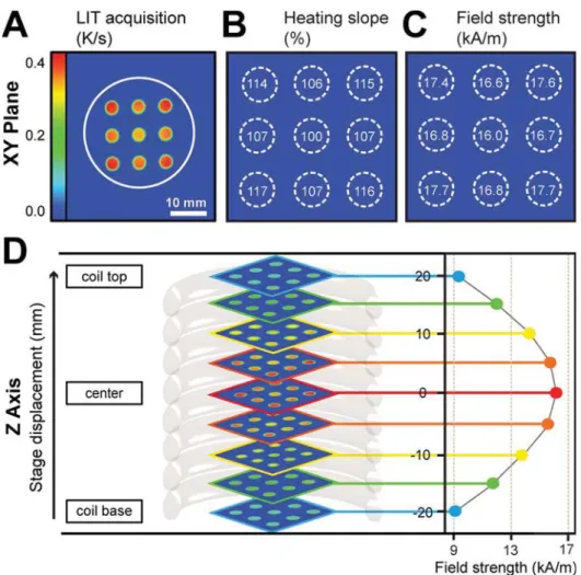
on size and coating). To do so, we loaded all nine cuvettes of the sample holder with the same amount and concentration of magnetic nanoparticles (16 mg/mL). A LIT recording of this layout immediately revealed the disparities in the magneticfield in the XY plane (Figure 2A), as the heating power of the nanoparticles, although identical in batch, material and concentration, was not identical in all cuvettes and we observed variations in the heating slopes (i.e., up to 17%, Figure 2.B) depending on the position of the sample. Given that thefield strength was previously measured with a capture-coil device in the central cuvette, LIT recordings enabled the back-calculation of thefield strength in every other respective cuvette (Figure 2C) using the magnetocrystalline anisotropy constant values estimated from the SAR values obtained from the sample in the central cuvette.
To provide a more extensive impression of the AMF strength within the entire coil, the holder was moved through the coil along the Z axis, while LIT acquisitions were continuously made at every increment (i.e., 5 mm,Figure 2D). Once again, these data were compiled in accordance with their spatial coordinates. The field intensity along the coil was also calculated with the pick-up coil: The results and a comparison with the theoretical ones are reported in the Supporting Information, Figure S4.
Figure 2. Inhomogeneities in the alternating magnetic field can be visualized by LIT. Magnetic field inhomogeneities will unavoidably lead to different results (e.g., while repositioning the sample). By using LIT, these variations can be visually rendered over the XY plane. This is done by loading identical nanoparticle solutions in all sample cuvettes and investigating their thermal signatures (A). Discrepancies in the heating profiles (B) are thus revealed, and are used to calculate the magneticfield strength in the respective cuvettes (C). For variations in the Z axis, the procedure is repeated while gradually displacing the sample holder in the coil (D). In this case thefield is calculated at each height for the central cuvette.
4.3. ILP Dependence on the Magnetic Field Strength. A precise knowledge of the AMF distribution within the coil is fundamental for an accurate determination of SAR. Never-theless, this parameter strongly depends on the field strength.33,64 Therein, the ILP was introduced by Kallumadil and colleagues39 in 2009 as a move toward a system-independent parameter and was intended to facilitate comparison between studies. Although the ILP has been used frequently in the literature, the degree to which it experimentally varies over a broader selection offield strengths is still an open topic of investigation.51 Therefore, in a preliminary trial, we investigated the SAR and ILP values of custom-made SPIONs (Figure 3A,B; seeSupporting Informa-tion for details on size and coating) as a function of field strength while keeping the frequency constant. Indeed, a dependence of the ILP on the magneticfield was observed in this series of measurements (Figure 3B). In particular, the ILP was not constant and exhibited a tendency to increase when the magnetic field strength decreased. To validate these results, simulations (Figure 3A,B) and FOC measurements ( Support-ing Information, Figure S5) were performed and compared to
the recorded values. These data were in good agreement with the experimentally measured values, and confirmed that the variations in the ILP are a consequence of thefield-dependent magnetic susceptibility of the nanoparticles.39,41In this regard, the LRT predicts that the susceptibility, as shown ineqs 4and 5, depends on the applied magneticfield, as well as on the size distribution.
We furthermore investigated the thermal behavior of SPIONs of commercial origin. Obtained by aqueous coprecipitation from iron salt precursors with a base, these SPIONs exhibited a drastically different size (distribution) and shape from the custom-made SPIONs synthesized by thermal decomposition (see Supporting Information for TEM micro-graphs). The experiments were performed on three nominally identical samples that all originated from the same supplier but were from different production batches. These suspensions were aliquoted at identical concentrations and their thermal properties were again measured as a function of the field strength (i.e., from 2.6 kA/m up to 13.9 kA/m). Again, ILP values exhibited a similar behavior as observed previously, with an overall increase in relation to a decreasing magnetic field Figure 3. Correlating experimental SAR and ILP values (LIT) to mathematical simulations (MS) as a function of the magnetic field strength. The thermal behavior of SPIONs is strongly dependent on the strength of the AMF to which they are exposed. This is reflected particularly well by the SAR (A) and ILP values (B) collected at different field strengths by LIT. Experimental values are shown individually (n = 9) and expressed in terms of their average (dashed line)± 1 SD (bars).
Figure 4. Commercial nanoparticles, field-dependent heating power and batch-to-batch variations. Identical measurements were performed as a function of the magneticfield strength, revealing the dependence of this factor on both the SAR (A) and the ILP (B), the latter exhibiting a continuous rise when approaching low AMF strengths. Moreover, these results highlight that SPIONs, even when produced under identical synthetic conditions, exhibit variations between batches. Experimental values are shown individually (n = 3) and expressed in terms of their average (dashed line)± 1 SD (bars).
strength (Figure 4B). Given the absolute ILP values, it should be noted that the recorded data related to previously reported results on the same nanoparticles (i.e., between 1.31 and 2.67 nHm2/kg),39
in particular when a comparable field range was applied (i.e., around 5−6 kA/m).
Finally, another important source of variability was high-lighted in these measurements: that nanoparticle batches, despite having been made under identical conditions, may vary considerably in their heating power. Indeed, from the SAR and ILP values recorded from these apparently identical samples (seeFigure 4A,B and Supporting Information, Figure S6, for FOC measurements), significant batch-to-batch variations of up to 30% were evident. These discrepancies, observed previously by Kallumadil and colleagues,39were ultimately associated with differences in the physical properties of the batches. In particular, while TEM micrographs showed that all samples exhibited fairly similar structures (Supporting Information), their hydrodynamic diameters measured by DLS were different, being 57± 4 nm (sample 1), 50 ± 2 (sample 2) and 39.6 ± 0.9 nm (sample 3), respectively. This shows that particles originating from the same synthetic method exhibit different physical properties, e.g. their hydrodynamic diameters, and that these divergences fundamentally relate to the heating abilities of the SPIONs.
5. CONCLUSIONS
Although magnetic nanoparticles and their applications are on the rise, their translation to the clinic still remains limited. The reason for this might lie in the difficulties related to improving the chemical design of the nanoparticles in terms of synthetic reproducibility, biocompatibility, and thermal efficiency. In order to do this, correct analysis of their heating behavior is imperative. In this respect, we have recently introduced lock-in thermography (LIT) as a new reliable technique for quantifying the heating properties of SPIONs in different colloidal states and at different concentrations.47,52The present work discusses the theory behind LIT and gives a detailed description on how this technique can be implemented to investigate critical aspects that can impair quantification of the heating power. The effect of magnetic field strength has been evaluated, both in regard to spatial inhomogeneities and its relation to the ILP. Indeed we have shown that discrepancies between ILP values as a function of magnetic field strength can be substantial. Nevertheless, due to the difficulty of providing a system-independent analytical solution to this query, the authors still believe that the ILP can represent a very relatable comparative unit, provided that each value is correlated by thefield strength used in a given study and that a series of ILP values are given for a specific particle batch. Given these insights, we hope that these notions will lead to more relatable results among groups, and consequently a higher degree of consensus within the community on which materials are more suitable for future applications.
■
ASSOCIATED CONTENT*
S Supporting InformationThe Supporting Information is available free of charge on the ACS Publications websiteat DOI:10.1021/acs.jpcc.7b09094.
Details on SPIONs synthesis and characterization, magnetic size distribution, XRD data, magnetic field inhomogeneity, andfiber optic cable measurements on SPIONs (PDF)
■
AUTHOR INFORMATIONCorresponding Authors
*(A.P.-F.) E-mail:alke.fi[email protected]. *(M.L.) E-mail:[email protected]. *(M.B.) E-mail:[email protected]. ORCID Marco Lattuada:0000-0001-7058-9509 Alke Petri-Fink:0000-0003-3952-7849 Present Address
∥Marine Science Institute and Department of Molecular, Cell &
Developmental Biology, University of California, 3154 Marine Biotechnology Building, Santa Barbara, California 93106, United States.
Author Contributions
‡C.A.M. and F.C. contributed equally. The manuscript was
written through contributions of all authors. All authors have given approval to thefinal version of the manuscript.
Notes
The authors declare no competingfinancial interest.
#
These authors are joint senior authors.
■
ACKNOWLEDGMENTSThis work was supported by the Swiss National Science Foundation (159803 and PP00P2_159258), the National Center of Competence in Research Bio-Inspired Materials, the Commission for Technology and Innovation (Project 18083.1 PFNM-NM), the Adolphe Merkle Foundation, the University of Fribourg and the Zurich University of Applied Sciences (ZHAW). The support of the Dr. Alfred Bretscher Fund is gratefully acknowledged, and access to TEM was kindly provided by the Microscopy Imaging Centre of the University of Bern. Access to VSM was kindly provided by Prof. Ann M. Hirt from the Institute for Geophysics of the ETH Zurich.
■
REFERENCES(1) Laurent, S.; Dutz, S.; Häfeli, U. O.; Mahmoudi, M. Magnetic Fluid Hyperthermia: Focus on Superparamagnetic Iron Oxide Nanoparticles. Adv. Colloid Interface Sci. 2011, 166, 8−23.
(2) Park, J.; An, K.; Hwang, Y.; Park, J.-G.; Noh, H.-J.; Kim, J.-Y.; Park, J.-H.; Hwang, N.-M.; Hyeon, T. Ultra-Large-Scale Syntheses of Monodisperse Nanocrystals. Nat. Mater. 2004, 3, 891−895.
(3) Gupta, A. K.; Gupta, M. Synthesis and Surface Engineering of Iron Oxide Nanoparticles for Biomedical Applications. Biomaterials 2005, 26, 3995−4021.
(4) Lattuada, M.; Hatton, T. A. Functionalization of Monodisperse Magnetic Nanoparticles. Langmuir 2007, 23, 2158−2168.
(5) Lee, N.; Yoo, D.; Ling, D.; Cho, M. H.; Hyeon, T.; Cheon, J. Iron Oxide Based Nanoparticles for Multimodal Imaging and Magneto-responsive Therapy. Chem. Rev. 2015, 115, 10637−10689.
(6) Périgo, E. A.; Hemery, G.; Sandre, O.; Ortega, D.; Garaio, E.; Plazaola, F.; Teran, F. J. Fundamentals and Advances in Magnetic Hyperthermia. Appl. Phys. Rev. 2015, 2, 041302.
(7) Hofmann-Amtenbrink, M.; von Rechenberg, B.; Hofmann, H. Superparamagnetic Nanoparticles for Biomedical Applications. Nano-structured Materials for Biomedical Applications 2009, 2, 119−149.
(8) Pankhurst, Q. A.; Connolly, J.; Jones, S. K.; Dobson, J. Applications of Magnetic Nanoparticles in Biomedicine. J. Phys. D: Appl. Phys. 2003, 36, R167−R181.
(9) Thiesen, B.; Jordan, A. Clinical Applications of Magnetic Nanoparticles for Hyperthermia. Int. J. Hyperthermia 2008, 24, 467− 474.
(10) Johannsen, M.; Gneveckow, U.; Eckelt, L.; Feussner, A.; Waldöfner, N.; Scholz, R.; Deger, S.; Wust, P.; Loening, S. A.; Jordan, A. Clinical Hyperthermia of Prostate Cancer Using Magnetic
Nanoparticles: Presentation of a New Interstitial Technique. Int. J. Hyperthermia 2005, 21, 637−647.
(11) Jordan, A.; Scholz, R.; Wust, P.; Fähling, H.; Felix, R. Roland Felix. Magnetic Fluid Hyperthermia (MFH): Cancer Treatment with AC Magnetic Field Induced Excitation of Biocompatible Super-paramagnetic Nanoparticles. J. Magn. Magn. Mater. 1999, 201, 413− 419.
(12) Mody, V. V.; Singh, A.; Wesley, B. Basics of Magnetic Nanoparticles for Their Application in the Field of Magnetic Fluid Hyperthermia. Eur. J. Nanomed. 2013, 5, 11−21.
(13) Neuberger, T.; Schöpf, B.; Hofmann, H.; Hofmann, M.; Von Rechenberg, B. Superparamagnetic Nanoparticles for Biomedical Applications: Possibilities and Limitations of a New Drug Delivery System. J. Magn. Magn. Mater. 2005, 293, 483−496.
(14) Bonnaud, C.; Monnier, C. A.; Demurtas, D.; Jud, C.; Vanhecke, D.; Montet, X.; Hovius, R.; Lattuada, M.; Rothen-Rutishauser, B.; Petri-Fink, A. The Insertion of Nanoparticle Clusters into Vesicle Bilayers. ACS Nano 2014, 8, 3451−3460.
(15) Amstad, E.; Kohlbrecher, J.; Müller, E.; Schweizer, T.; Textor, M.; Reimhult, E. Triggered Release from Liposomes through Magnetic Actuation of Iron Oxide Nanoparticle Containing Membranes. Nano Lett. 2011, 11, 1664−1670.
(16) Hernández, R.; Sacristán, J.; Asín, L.; Torres, T. E.; Ibarra, M. R.; Goya, G. F.; Mijangos, C. Magnetic Hydrogels Derived from Polysaccharides with Improved Specific Power Absorption: Potential Devices for Remotely Triggered Drug Delivery. J. Phys. Chem. B 2010, 114, 12002−12007.
(17) Mehdaoui, B.; Meffre, A.; Carrey, J.; Lachaize, S.; Lacroix, L. M.; Gougeon, M.; Chaudret, B.; Respaud, M. Optimal Size of Nano-particles for Magnetic Hyperthermia: A Combined Theoretical and Experimental Study. Adv. Funct. Mater. 2011, 21, 4573−4581.
(18) Rosensweig, R. E. Heating Magnetic Fluid with Alternating Magnetic Field. J. Magn. Magn. Mater. 2002, 252, 370−374.
(19) Munoz-Menendez, C.; Conde-Leboran, I.; Baldomir, D.; Chubykalo-Fesenko, O.; Serantes, D. The Role of Size Polydispersity in Magnetic Fluid Hyperthermia: Average vs. Local Infra/over-Heating Effects. Phys. Chem. Chem. Phys. 2015, 17, 27812−27820.
(20) Filippousi, M.; Angelakeris, M.; Katsikini, M.; Paloura, E.; Efthimiopoulos, I.; Wang, Y.; Zamboulis, D.; Van Tendeloo, G. Surfactant Effects on the Structural and Magnetic Properties of Iron Oxide Nanoparticles. J. Phys. Chem. C 2014, 118, 16209−16217.
(21) Serantes, D.; Simeonidis, K.; Angelakeris, M.; Chubykalo-Fesenko, O.; Marciello, M.; Morales, M. P.; Baldomir, D.; Martinez-Boubeta, C. Multiplying Magnetic Hyperthermia Response by Nanoparticle Assembling. J. Phys. Chem. C 2014, 118, 5927−5934.
(22) Urtizberea, A.; Natividad, E.; Arizaga, A.; Castro, M.; Mediano, A. Specific Absorption Rates and Magnetic Properties of Ferrofluids with Interaction Effects at Low Concentrations. J. Phys. Chem. C 2010, 114, 4916−4922.
(23) Wildeboer, R. R.; Southern, P.; Pankhurst, Q. A. On the Reliable Measurement of Specific Absorption Rates and Intrinsic Loss Parameters in Magnetic Hyperthermia Materials. J. Phys. D: Appl. Phys. 2014, 47, 495003.
(24) De La Presa, P.; Luengo, Y.; Multigner, M.; Costo, R.; Morales, M. P.; Rivero, G.; Hernando, A. Study of Heating Efficiency as a Function of Concentration, Size, and Applied Field in γ-Fe2O3 Nanoparticles. J. Phys. Chem. C 2012, 116, 25602−25610.
(25) Andreu, I.; Natividad, E. Accuracy of Available Methods for Quantifying the Heat Power Generation of Nanoparticles for Magnetic Hyperthermia. Int. J. Hyperthermia 2013, 29, 739−751.
(26) Huang, S.; Wang, S.-Y.; Gupta, A.; Borca-Tasciuc, D.-A.; Salon, S. J. On the Measurement Technique for Specific Absorption Rate of Nanoparticles in an Alternating Electromagnetic Field. Meas. Sci. Technol. 2012, 23, 035701.
(27) Wang, S. Y.; Huang, S.; Borca-Tasciuc, D. A. Potential Sources of Errors in Measuring and Evaluating the Specific Loss Power of Magnetic Nanoparticles in an Alternating Magnetic Field. IEEE Trans. Magn. 2013, 49, 255−262.
(28) Conde-Leboran, I.; Baldomir, D.; Martinez-Boubeta, C.; Chubykalo-Fesenko, O.; Del Puerto Morales, M.; Salas, G.; Cabrera, D.; Camarero, J.; Teran, F. J.; Serantes, D. A Single Picture Explains Diversity of Hyperthermia Response of Magnetic Nanoparticles. J. Phys. Chem. C 2015, 119, 15698−15706.
(29) Lemal, P.; Geers, C.; Rothen-Rutishauser, B.; Lattuada, M.; Petri-Fink, A. Measuring the Heating Power of Magnetic Nano-particles: An Overview of Currently Used Methods. Mater. Today Proc., in press.
(30) Natividad, E.; Castro, M.; Mediano, A. Adiabatic vs. Non-Adiabatic Determination of Specific Absorption Rate of Ferrofluids. J. Magn. Magn. Mater. 2009, 321, 1497−1500.
(31) Mac Oireachtaigh, C.; Fannin, P. C. Investigation of the Non-Linear Loss Properties of Magnetic Fluids Subject to Large Alternating Fields. J. Magn. Magn. Mater. 2008, 320, 871−880.
(32) Ahrentorp, F.; Astalan, A. P.; Jonasson, C.; Blomgren, J.; Qi, B.; Mefford, O. T.; Yan, M.; Courtois, J.; Berret, J. F.; Fresnais, J.; Sandre, O.; Dutz, S.; Müller, R.; Johansson, C. Sensitive High Frequency AC Susceptometry in Magnetic Nanoparticle Applications. AIP Conf. Proc. 2010, 1311, 213−223.
(33) Carrey, J.; Mehdaoui, B.; Respaud, M. Simple Models for Dynamic Hysteresis Loop Calculations of Magnetic Single-Domain Nanoparticles: Application to Magnetic Hyperthermia Optimization. J. Appl. Phys. 2011, 109, 083921.
(34) Beković, M.; Trlep, M.; Jesenik, M.; Goričan, V.; Hamler, A. An Experimental Study of Magnetic-Field and Temperature Dependence on Magnetic Fluid’s Heating Power. J. Magn. Magn. Mater. 2013, 331, 264−268.
(35) Zhong, J.; Liu, W.; Du, Z.; César de Morais, P.; Xiang, Q.; Xie, Q. A Noninvasive, Remote and Precise Method for Temperature and Concentration Estimation Using Magnetic Nanoparticles. Nano-technology 2012, 23, 075703.
(36) Zhong, J.; Liu, W.; Jiang, L.; Yang, M.; Morais, P. C. Real-Time Magnetic Nanothermometry: The Use of Magnetization of Magnetic Nanoparticles Assessed under Low Frequency Triangle-Wave Magnetic Fields. Rev. Sci. Instrum. 2014, 85, 094905.
(37) Pi, S.; Liu, W.; Zhong, J.; Xiang, Q.; Morais, P. C. Towards Real-Time and Remote Magnetonanothermometry with Temperature Accuracy Better than 0.05 K. Sens. Actuators, A 2015, 234, 263−268. (38) Vollmer, M.; Möllmann, K.-P. Infrared Thermal Imagings: Fundamentals, Research and Applications; John Wiley & Sons: Weinheim, Germany, 2010.
(39) Kallumadil, M.; Tada, M.; Nakagawa, T.; Abe, M.; Southern, P.; Pankhurst, Q. A. Suitability of Commercial Colloids for Magnetic Hyperthermia. J. Magn. Magn. Mater. 2009, 321, 1509−1513.
(40) Hergt, R.; Dutz, S.; Röder, M. Effects of Size Distribution on Hysteresis Losses of Magnetic Nanoparticles for Hyperthermia. J. Phys.: Condens. Matter 2008, 20, 385214.
(41) Dutz, S.; Hergt, R. Magnetic Nanoparticle Heating and Heat Transfer on a Microscale: Basic Principles, Realities and Physical Limitations of Hyperthermia for Tumour Therapy for Tumour Therapy. Int. J. Hyperthermia 2013, 29, 790−800.
(42) Bordelon, D. E.; Goldstein, R. C.; Nemkov, V. S.; Kumar, A.; Jackowski, J. K.; Deweese, T. L.; Ivkov, R. Magnetic Fields With Enhanced Uniformity for Biomedical Applications. IEEE Trans. Magn. 2012, 48, 47−52.
(43) Stauffer, P. R.; Sneed, P. K.; Hashemi, H.; Phillips, T. L. Practical Induction Heating Coil Designs for Clinical Hyperthermia with Ferromagnetic Implants. IEEE Trans. Biomed. Eng. 1994, 41, 17− 28.
(44) Busse, G.; Wu, D.; Karpen, W. Thermal Wave Imaging with Phase Sensitive Modulated Thermography. J. Appl. Phys. 1992, 71, 3962−3965.
(45) Kuo, P. K.; Ahmed, T.; Jin, H.; Thomas, R. L. Phase-Locked Image Acquisition in Thermography. Proc. SPIE 1988, 41−47.
(46) Breitenstein, O.; Warta, W.; Langenkamp, M. Lock-in Thermography: Basics and Use for Evaluating Electronic Devices and Materials; Springer-Verlag: Berlin and Heidelberg, Germany, 2010.
(47) Monnier, C. A.; Lattuada, M.; Burnand, D.; Crippa, F.; Martinez-Garcia, J. C.; Hirt, A. M.; Rothen-Rutishauser, B.; Bonmarin, M.; Petri-Fink, A. A Lock-in-Based Method to Examine the Thermal Signatures of Magnetic Nanoparticles in the Liquid, Solid and Aggregated States. Nanoscale 2016, 8, 13321−13332.
(48) Rosensweig, R. E. E. Ferrohydrodynamics; Dover Publications, Inc.: New York, 1985.
(49) Lak, A.; Kraken, M.; Ludwig, F.; Kornowski, A.; Eberbeck, D.; Sievers, S.; Litterst, F. J.; Weller, H.; Schilling, M. Size Dependent Structural and Magnetic Properties of FeO-Fe3O4 nanoparticles. Nanoscale 2013, 5, 12286−12295.
(50) Shliomis, M. I.; Stepanov, V. I. Theory of the Dynamic Susceptibility of Magnetic Fluids: Relaxation Phenomena in Condensed Matter; John Wiley & Sons: 1994.
(51) Coïsson, M.; Barrera, G.; Celegato, F.; Martino, L.; Vinai, F.; Martino, P.; Ferraro, G.; Tiberto, P. Specific Absorption Rate Determination of Magnetic Nanoparticles through Hyperthermia Measurements in Non-Adiabatic Conditions. J. Magn. Magn. Mater. 2016, 415, 2−7.
(52) Lemal, P.; Geers, C.; Monnier, C. A.; Crippa, F.; Daum, L.; Urban, D. A.; Rothen-Rutishauser, B.; Bonmarin, M.; Petri-Fink, A.; Moore, T. L. Lock-in Thermography as a Rapid and Reproducible Thermal Characterization Method for Magnetic Nanoparticles. J. Magn. Magn. Mater. 2017, 427, 206−211.
(53) Gokhale, P. Mixed Convective Heat Transfer and Evaporation at the Air-Water Interface. Ph.D. Thesis, Clemson University: 2007.
(54) Liu, J.; Yang, W.; Dai, J. Research on Thermal Wave Processing of Lock- in Thermography Based on Analyzing Image Sequences for NDT. Infrared Phys. Technol. 2010, 53, 348−357.
(55) Krapez, J.-C. Compared Performances of Four Algorithms Used for Modulation Thermography. Quantitative Infrared Thermography 1998, 148−153.
(56) Gupta, R.; Breitenstein, O. Temperature Drift Correction for Fast Lock-in Infrared Thermography. 21st European Photovoltaic Solar Energy Conference 2006, 332−335.
(57) Sun, S.; Zeng, H. Size-Controlled Synthesis of Magnetite Nanoparticles. J. Am. Chem. Soc. 2002, 124, 8204−8205.
(58) Burnand, D.; Monnier, C. A.; Redjem, A.; Schaefer, M.; Rothen-Rutishauser, B.; Kilbinger, A.; Petri-Fink, A. Catechol-Derivatized Poly(vinyl Alcohol) as a Coating Molecule for Magnetic Nanoclusters. J. Magn. Magn. Mater. 2015, 380, 157−162.
(59) Amstad, E.; Gillich, T.; Bilecka, I.; Textor, M.; Reimhult, E. Ultra-Stable Iron Oxide Nanoparticle Colloidal Suspensions Using Dispersants with Catechol Derived Anchor Groups. Nano Lett. 2009, 9, 4042−4048.
(60) Boutry, S.; Forge, D.; Burtea, C.; Mahieu, I.; Murariu, O.; Laurent, S.; Vander Elst, L.; Muller, R. N. How to Quantify Iron in an Aqueous or Biological Matrix: A Technical Note. Contrast Media Mol. Imaging 2009, 4, 299−304.
(61) Michen, B.; Geers, C.; Vanhecke, D.; Endes, C.; Rothen-Rutishauser, B.; Balog, S.; Petri-Fink, A. Avoiding Drying-Artifacts in Transmission Electron Microscopy: Characterizing the Size and Colloidal State of Nanoparticles. Sci. Rep. 2015, 5, 9793.
(62) Monnier, C. A.; Bonmarin, M.; Crippa, F.; Geers, C.; Petri-Fink, A. Sample Holder and Lock-in Thermography System with Such. US 62/331,017 May 03, 2016.
(63) Gesellshaft, V. VDI Heat Atlas.; Springer-Verlag: Berlin and Heidelberg, Germany, 2010.
(64) Serantes, D.; Baldomir, D.; Martinez-Boubeta, C.; Simeonidis, K.; Angelakeris, M.; et al. Influence of Dipolar Interactions on Hyperthermia Properties of Ferromagnetic Particles. J. Appl. Phys. 2010, 108, 073918.