Petroleum
hydrocarbon mineralization in anaerobic
laboratory
aquifer columns
Daniel
Hunkeler, Dominik Jorger
¨
1,
Katharina
Haberli,
¨
Patrick
Hohener
¨
),
Josef Zeyer
Swiss Federal Institute of Technology ETH( ), Institute of Terrestrial Ecology, Soil Biology, CH-8952 Schlieren, Switzerland
Abstract
The anaerobic biodegradation of hydrocarbons at mineral oil contaminated sites has gathered increasing interest as a naturally occurring remediation process. The aim of this study was to investigate biodegradation of hydrocarbons in laboratory aquifer columns in the absence of O2and
NOy3
, and to calculate a mass balance of the anaerobic biodegradation processes. The laboratory columns contained aquifer material from a diesel fuel contaminated aquifer. They were operated at 258C for 65 days with artificial groundwater that contained only SO2y and CO
4 2 as externally
supplied oxidants. After 31 days of column operation, stable concentration profiles were found for most of the measured dissolved species. Within 14 h residence time, about 0.24 mM SO42y were
consumed and dissolved Fe IIŽ . Žup to 0.012 mM ,. Mn IIŽ . Žup to 0.06 mM ,. and CH4Žup to 0.38
mM were produced. The alkalinity and the dissolved inorganic carbon. ŽDIC concentration.
increased and the DIC became enriched in 13C. In the column, n-alkanes were selectively removed while branched alkanes persisted, suggesting a biological degradation. Furthermore, based on changes of concentrations of aromatic compounds with similar physical–chemical properties in the effluent, it was concluded that toluene, p-xylene and naphthalene were degraded. A carbon mass balance revealed that 65% of the hydrocarbons removed from the column were recovered as DIC, 20% were recovered as CH4, and 15% were eluted from the column. The calculations indicated that hydrocarbon mineralization coupled to SO4
2y
reduction and methanogenesis con-tributed in equal proportions to the hydrocarbon removal. Hydrocarbon mineralization coupled to
)
Corresponding author. Tel.: q41-1-633-6042; fax: q41-1-633-1122; e-mail: [email protected]
1
Present address: BMG Engineering AG, CH-8952 Schlieren, Switzerland.
Fe IIIŽ .and MnŽIV. reduction was of minor importance. DIC, alkalinity, and stable carbon isotope balances were shown to be a useful tool to verify hydrocarbon mineralization.
Keywords: Intrinsic bioremediation; Petroleum hydrocarbons; Groundwater; Stable carbon isotopes; Methano-genesis; Sulfate reduction
1. Introduction
Ž
Contamination of aquifers with petroleum hydrocarbons designated as hydrocarbons .
throughout the text is a widespread environmental problem that has led to the development of several remediation technologies. In situ bioremediation has found special attention because it ideally leads to complete mineralization of the hydrocarbons
Ž
without expensive excavation of the contaminated zone Battermann, 1983; US National .
Research Council, 1993 . In aquifers contaminated with hydrocarbons, indigenous Ž microbial populations that can mineralize hydrocarbons are usually established Thomas
.
and Ward, 1994 . In the contaminated zones, anaerobic conditions often prevail because
Ž .
the O demand exceeds the O supply Bouwer, 1992 . Therefore, engineered in situ2 2
Ž
bioremediation schemes are usually based on an external supply of oxidants O , H O ,2 2 2
y
. Ž
andror NO3 to increase the aerobic and denitrifying mineralization rates Battermann, .
1983; Hutchins et al., 1991; Hunkeler et al., 1995 .
During the last years, however, it has been shown in laboratory studies that the mineralization of various aromatic and aliphatic hydrocarbons can also be coupled to the
Ž . Ž . 2y
reduction of Fe III , Mn IV , SO4 and CO as summarized by Holliger and Zehnder2
Ž1996 . Field studies suggest that biodegradation under these redox conditions can. Ž
significantly contribute to the removal of hydrocarbons from aquifers Baedecker et al., .
1993; Borden et al., 1995; Thierrin et al., 1995 . In an aquifer contaminated with crude
Ž .
oil, which was not treated by active measures Essaid et al., 1995 , a greater amount of Ž .
hydrocarbon was degraded under anaerobic conditions 60% than under aerobic condi-Ž .
tions 40% due to the limited supply of O . The authors of the study estimated that2
about 19% of the hydrocarbon degradation was coupled to Fe reduction, 5% was coupled to Mn reduction, and 36% was coupled to methanogenesis. We reported on an aquifer at Menziken, Switzerland, which was contaminated with diesel fuel and treated
y
Ž . Ž . by adding O , NO2 3 and nutrients. Despite these additions, dissolved Fe II , Mn II and CH4 were found in the contaminated zone, and the SO42y concentration decreased, indicating that hydrocarbons were mineralized under Fe-reducing, Mn-reducing, SO42y
-Ž .
reducing, and methanogenic conditions as well Hunkeler et al., 1995 . In the field, however, it is difficult to demonstrate that the consumption of oxidants is coupled to the mineralization of hydrocarbons, and that a related amount of hydrocarbons is removed ŽMadsen, 1991; Hunkeler et al., 1997 . Laboratory aquifer columns allow an ex situ. verification of hydrocarbon mineralization, since complete carbon mass balance can be established. Hydrocarbon mineralization under aerobic and denitrifying conditions in the contaminated aquifer at Menziken was verified previously using laboratory aquifer
Ž .
In this study, hydrocarbon mineralization in the absence of O and NOy
was
2 3
investigated using laboratory aquifer columns. The objectives of the investigations were Ž .1 to study the evolution of Fe-reducing, Mn-reducing, SO42y-reducing, and
Ž .
methanogenic conditions; 2 to relate the consumption of oxidants and the production Ž .
of reduced species to the production of dissolved inorganic carbon DIC based on DIC, Ž .
alkalinity, and stable carbon isotope balances; 3 to evaluate the contribution of the Ž .
various redox processes to hydrocarbon mineralization; 4 to perform a carbon mass Ž .
balance; and 5 to determine which hydrocarbons were degraded.
2. Materials and methods
2.1. Experimental set-up
Ž . Ž
The columns Fig. 1A were identical to those described elsewhere Hess et al., .
1996 . They had an inner diameter of 5 cm and a total length of 47 cm. Sampling ports Ž
were made of stainless-steel hypodermic needles ID 1.5 mm, Unimed, Geneva,
. Ž
Switzerland placed into GC septa Injection Rubber Plugs Part. No. 201-35584, .
Shimadzu, Japan that were fitted into 4.8 mm borings. The aquifer material used to fill the columns was excavated from a diesel fuel contaminated aquifer in Menziken, Switzerland in which Mn-reducing, Fe-reducing, SO2y-reducing and methanogenic
4
Ž .
conditions were observed Hunkeler et al., 1995 . The excavated material was sieved Ž- 4.5 mm . Dried material consisted of - 1% silt and clay - 0.02 mm , 13% fine. Ž .
Ž . Ž .
sand 0.02–0.2 mm and 86% coarse sand 0.2–4.5 mm and contained about 40% wrw
Ž .
carbonates mainly CaCO . The concentration of weathered diesel fuel was 950 mg3
y1
Ž .
kg dry weight. The material was amended with fresh diesel fuel Esso, Switzerland to yield a total hydrocarbon concentration of 1410 mg kgy1
dry weight. Water-saturated material was homogenized by vigorous stirring and subsequently used to fill two columns. After allowing the material to settle for 2 days, the column filling covered a length of 39 cm and had a total porosity of 0.21, calculated from the volume, weight and density of the material. The hydrocarbon-amended aquifer material, which was used to fill the columns, is denoted as initial aquifer material throughout the text.
The columns were operated at 25 " 0.58C in a vertical position under upflow
Ž y1.
conditions flow rates of 10.0 " 0.5 ml h . Artificial groundwater consisted of 6.00 mM NaHCO , 0.20 mM Na SO and 0.05 mM MgSO P 7H O in distilled water. It was3 2 4 4 2
Ž .
autoclaved at 1208C for 20 min. Sterile solutions of CaCl P 2H O 0.25 mM final conc.2 2
Ž .
and KH PO2 4 0.01 mM final conc. were added after autoclaving. The pH was adjusted to 7.5 using 1 M sterile HCl. Concentrations of dissolved oxygen were lowered to - 0.1 mg ly1
by passing the artificial groundwater through silicone tubes of 2 m length in a
Ž .
bottle that was continuously flushed with N2 Zeyer et al., 1986 . Two identical columns were operated over 65 days. Transport parameters were characterized by adding 1 mM NaBr to the artificial groundwater at day 39 of operation. Breakthrough curves were obtained by measuring Bry
-concentrations and analyzed using the computer code
Ž .
average groundwater residence time of 14 h, and a peclet number of 1.6. Comparable transport parameters and concentration profiles of dissolved species were observed in both columns.
2.2. Sampling and analysis of dissolÕed species
Depending on the chemical species, 3 to 7 concentration profiles were measured Ž 13 . during 65 days of column operation. The stable carbon isotope composition d C of the DIC was measured once on day 48. Water samples were taken using 10 ml glass
Ž .
syringes equipped with stainless steel valves Merck, Dietikon, Switzerland to avoid loss of volatile compounds. The syringes were filled without headspace at the same rate as the flow rate in the column. Samples were taken in the inverse direction to the water flow starting at the column outlet to minimize the disturbance. Unless stated otherwise, water samples from the columns were filtered using 0.22 mm Millipore PTFE filters ŽMillipore, Volketswil, Switzerland . The sums of Ca, Mg, Fe and Mn in the form of.
Ž . Ž . Ž . free ions and complexes with redox state qII are denoted as Ca II , Mg II , Fe II and
Ž . Ž . y 2y
Mn II . Dissolved S yII corresponds to the sum of H S, HS2 and S . For the Ž . Ž . Ž . Ž .
measurement of dissolved Ca II , Mg II , Fe II , Mn II , and dissolved organic carbon ŽDOC , samples were acidified with distilled HNO to yield a final concentration of. 3
2y y y
Ž . Ž .
0.025 M HNO . Concentrations of SO3 4 , Cl , Br , Ca II and Mg II were determined
Ž .
using a Dionex DX-100 ion chromatograph Dionex, Sunnyvale, USA . Ammonium and
Ž . Ž .
dissolved S yII were measured colorimetrically APHA, 1989 . Fe and Mn were Ž
quantified by atomic absorption spectroscopy AAS; Varian SpectrAA 400, Varian .
Techtron, Springvale, Australia . Since the solubility of amorphous FeOOH in the
Ž .
absence of strong ligands is - 1 mM at pH 6 to 8 Stumm and Morgan, 1996 , it was assumed that the measured concentration of dissolved Fe corresponds to the concentra-tion of Fe2q in the form of free ions and complexes in the original sample. DOC
Ž .
concentrations were determined with a Horiba TOC-analyzer Horiba, Kyoto, Japan . Before analysis, the acidified samples were vigorously bubbled with N2 to ensure complete stripping of DIC. It has to be taken into account that volatile hydrocarbons Že.g., monoaromatic compounds and volatile metabolites are stripped as well. Concen-. trations of dissolved CO2 and CH4 were determined using 10 ml glass syringes that were filled with 4 ml sample without contact with the atmosphere and an additional 2 ml N headspace. After shaking the syringes and equilibration for 4 h, the partial pressure2
Ž
of the gases were measured by gas chromatography Fisons Model 8000; Fisons,
. Ž .
Rodano, Italy on a HayeSep D column Alltech, Deerfield, IL at 708C with N as2
Ž .
carrier and a Carlo Erba thermal conductivity detector Fisons, Rodano, Italy . Concen-trations of dissolved gases were calculated from Henry’s law using the following Henry
y1 y1 Ž
constants at 258C: CO :0.0339 M atm2 , CH :0.00129 M atm4 Stumm and Morgan, .
1996 . Alkalinity was measured by potentiometric titration using Gran plots for
graphi-Ž . Ž .
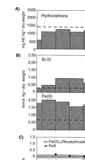
Fig. 1. A Schematic illustration of column that was operated in upright position. B Arithmetic mean of concentrations of dissolved species measured between days 31 and 65 and d13C of DIC measured at day 48.
The concentrations given at 0 cm column length corresponds to the concentrations measured in the bottle with the artificial groundwater. For DIC and the d13C of the DIC, no values are given at 0 cm column length
because the DIC concentration and d13C changed during the passage of the water through the silicone tube in
the gas exchange bottle. The concentrations given at 39 cm column length correspond to the concentrations measured in the effluent of the column.
Ž .
cal determination of the end point Stumm and Morgan, 1996 . The DIC concentration and pH was calculated based on the alkalinity and the concentration of dissolved CO2
ŽStumm and Morgan, 1996 ..
For stable carbon isotope analysis of the DIC, 10 ml of water were collected in glass syringes without headspace. The DIC was precipitated as BaCO by the addition of 0.13
Ž . Ž
ml of a CO -free NaOH solution 1.5 M and 0.4 ml of a CO -free BaCl solution 1.22 2 .
mM . After 10 h of equilibration, the sample was discharged from the syringe through a 0.22 mm Millipore PTFE filter. The filtrate was dried at 1058C for 12 h. The BaCO3 was converted to CO under a vacuum by the addition of H PO . The 13C:12C ratios
2 3 4
Ž
were measured with a Fisons Prism isotope-ratio mass spectrometer Fisons,
Mid-. Ž 13 .
dlewich, Cheshire, UK and are reported in the usual delta notation d C referenced to
Ž . Ž .
the PDB Peedee belemnite standard Coplen, 1996 .
To quantify the elution of hydrocarbons from the column, 80 to 420 ml sample were taken at the outlet of the column using 500 ml separatory funnels. The separatory funnels contained 5 to 10 ml pentane with 1-chloroctane as an internal standard and were chilled on ice to avoid evaporation of the pentane. The hydrocarbons were extracted into the pentane by vigorous shaking. The organic phase was analyzed by gas
Ž . Ž .
chromatography GC using a capillary Bregnard et al., 1996 as well as a packed
Ž .
separatory column Haner et al., 1995 . The packed column allowed separation of m-
¨
and p-xylene, which could not be separated on the capillary column. Hydrocarbons were identified and quantified using external standards. The peaks that could not be identified were quantified using the average response factor of the identified peaks. Some of the unidentified peaks may have consisted of volatile metabolites. Benzene could not be quantified due to poor separation from the solvent.
2.3. Sampling and analysis of column matrix
At day 65, the column operation was stopped, and one column was frozen at y188C. The frozen material was extruded and sliced as shown in Fig. 1A. The frozen slices were immediately transferred to an anaerobic chamber containing a N atmosphere. All data2
of compounds in the solid and water phase shown in the results section were obtained from this column.
Hydrocarbons were extracted by sonication using CH Cl as the solvent according to2 2
Ž .
the EPA method 3550 US Environmental Protection Agency, 1989 . The total hydro-carbon concentration and the concentration of single compounds were determined by
Ž .
capillary GC analysis of the extracts as described in detail by Bregnard et al. 1996 . For stable carbon isotope analysis of the weathered diesel fuel, contaminated aquifer material that had not been amended with fresh diesel fuel was extracted with CH Cl .2 2 The extract was evaporated to a constant weight, and 10 ml of the residue was combusted in an evacuated quartz tube at 9508C for 3 h using 1 g CuO as an oxidant. The CO2 that was produced was analyzed with a Fisons Optima isotope-ratio mass
Ž . 13
spectrometer Fisons, Middlewich, Cheshire, UK . The d C of the fresh diesel fuel was determined identically as that of the extracted hydrocarbons. For stable carbon isotope analysis of the carbonates in the aquifer material, a sample of aquifer material was ground, and the d13C was determined identically as that of the precipitated BaCO .
Ž .
FeS was extracted with 0.5 M HCl according to Heron et al. 1994 . The extraction
3q Ž
was performed at 258C to avoid oxidation of H S by Fe2 Von Gunten and Zobrist,
. Ž . Ž .
1993 . In the extracts, Fe II was analyzed using the phenanthroleine method and S yII
Ž .
using the methylene blue method APHA, 1989 .
Microbial cells were removed from aquifer solids by vortexing 1 g of aquifer material Ž
in 10-ml filtered artificial groundwater containing 0.1% Na P O4 2 7 Balkwill et al., .
1988 . The aquifer solids were allowed to settle down for 2 min; then, the cells in the supernatant were fixed, stained with DAPI and directly counted with a Zeiss Axioplan
Ž .
epifluorescence microscope Zeiss, Oberkochen, Germany as reported by Hahn et al. Ž1992 ..
2.4. Calculations
Ž .
Saturation calculations were performed with MICROQL Westall, 1986 using
stabil-Ž . Ž .
ity constants from Thorstenson and Plummer 1977 , Matsunaga et al. 1993 and
Ž .
Stumm and Morgan 1996 . The stability constants were corrected for temperature and ionic strength using the van’t Hoff equation and the Guntelberg approximation, respec-
¨
Ž .
tively Stumm and Morgan, 1996 . The consumption or production of dissolved species during 65 days of column operation was quantified by multiplying the difference between the average concentration in the effluent, and the inflow with the flow rate and Ž . the length of the operation time. The average concentration of hydrocarbons, S yII ,
Ž .
and Fe II in the solid phase after termination of column operation was obtained by multiplying the concentration in each slice with the weight of the slice, adding the amounts of all eight slices and dividing the sum by the total weight of the aquifer material. The total elution of DOC and dissolved hydrocarbons from the column was obtained by integrating the concentration vs. time curves of the effluent. The reported uncertainties of measured values are standard uncertainties determined according to
Ž .
International Organization for Standardization 1993 . Uncertainties on calculated values Ž
were estimated using the law of propagation of uncertainty International Organization .
for Standardization, 1993 .
3. Results
3.1. Concentrations of dissolÕed species
The average of the concentrations of dissolved species measured between days 31 and 65 are shown in Fig. 1B. Between days 31 and 65, the general shape of the concentration profiles remained constant. In the first 26 cm of the column, SO2y was
4
Ž .
almost completely consumed and the average S II concentrations were higher than 1
Ž . Ž .
mM Fig. 1B . The Fe II concentration was constant between 2 and 20 cm column Ž .
length, but increased at column length ) 20 cm. The Mn II , CH , alkalinity and DIC4 concentrations steadily increased with increasing column length. The d13C of the DIC
Ž .
increased by 3.1‰ Fig. 1 B . The pH increased until 14 cm column length and then decreased again.
For CH and CO , the partial pressures were calculated from the concentrations of4 2
dissolved gases and the Henry coefficients. The partial pressure of CH increased to 0.24
atm at the column end. The partial pressure of CO was 0.006 " 0.001 atm, and the2
partial pressure of N was 0.98 atm, assuming that the water was in equilibrium with2 respect to N at the column inlet, and N was neither consumed nor produced in the2 2 column. Thus, the total partial pressure of the dissolved gases increased to greater than 1 atm due to the production of CH . This increase explains the observed formation of gas4 bubbles in the aquifer material. The gas bubbles were mainly found at column lengths ) 20 cm.
3.2. Concentrations of inorganic species in solid phase and saturation calculations
Ž .
At the end of the column experiment, the highest S yII concentrations in the solid
Ž . Ž .
phase were found between 8 and 26 cm column length Fig. 2B while the Fe II concentrations were elevated by about 1.3 " 0.3 mmol kgy1
dry weight compared to the initial aquifer material over the entire length of the column. Saturation calculations were performed based on the measurements of dissolved species made between day 38 and 49 depending on the species. Samples were saturated with respect to FeS at sampling ports located at 8, 14 and 20 cm column length and saturated or oversaturated with respect to
Ž . Ž .
FeCO3 Siderite at 26, 35 and 39 cm column length Fig. 2C . Samples of all sampling
Ž . Ž
ports were undersaturated with respect to MnCO3 Rhodocrosite and MnS data not
. Ž .
shown . Furthermore, all samples were saturated with respect to CaCO3 Calcite and
Ž . Ž .
low-magnesium calcites, and undersaturated with respect to CaMg CO3 2 Dolomite and magnesium calcites containing more than 7% mole magnesium carbonate. Direct cell counts resulted in 6.7 " 1.0 P 107 cells gy1
dry aquifer material. No significant change between the cell numbers at the beginning and the end of the experiment was observed.
3.3. Concentrations of hydrocarbons
At the end of the experiment, total hydrocarbon concentrations in the solid phase were found to be lower than in the initial aquifer material in all slices between 0 and 35
Ž .
cm column length Fig. 2C . However, in the last slice, the total hydrocarbon concentra-tion was elevated. The largest decrease of the total hydrocarbon concentraconcentra-tion was observed in the first slice. In the initial aquifer material, n-alkanes as well as i-alkanes Žisoprenoid alkanes, e.g., farnesane, norpristane, pristane, phytane were present Fig.. Ž
.
3A . After 65 days of column operation, n-alkane concentrations were below the
Ž .
detection limit in all slices, while the i-alkanes were still present Fig. 3B . In total, 200
y1
Ž .
mg kg dry weight hydrocarbons were removed Table 1 . One third of the decrease of the hydrocarbon concentration in the column could be attributed to the removal of
n-alkanes, while the remaining two-thirds was due to the removal of unidentified
Ž . 13
compounds. The i-alkane concentration remained constant Table 1 . The d C of the weathered diesel fuel in the aquifer material was y29.7‰, the d13C of the added diesel
Ž . Ž .
Fig. 2. A Hydrocarbon concentration in the aquifer material before broken line and after 65 days of column
Ž . Ž . Ž . Ž .
operation. B S yII and Fe II concentration in the aquifer material before broken line and after 65 days of
Ž . Ž .
column operation. C Saturation indices of FeCO , FeS, CaCO3 3 and CaMg CO3 2 calculated from data measured between day 38 and 49. Positive values indicate oversaturation; negative values indicate undersatura-tion. The hatched areas correspond to the range of uncertainty of the calculations.
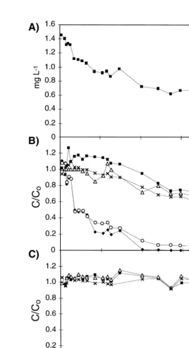
The concentration of the hydrocarbons detected in the effluent of the column was 1.5
y1
Ž . y1
mg l at day 1 Fig. 4A . It decreased to 0.7 mg l at day 20, and then remained at a constant level of 0.64 " 0.03 mg ly1
Approxi-Ž .
Fig. 3. GC analysis of hydrocarbons in the aquifer material at the start of the experiment A and in the aquifer
Ž .
material of slice 2–8 cm after 65 days of column operation B . UCM: unresolved complex mixture, 10–21:
Ž .
carbon numbers of n-alkanes, f s farnesane 2,6,10-trimethyldodecane , i-C16sC -isoprenoid alkane16 Ž2,6,10-trimethyltridecane , n s norpristane 2,6,10-trimethylpentadecane , pr s pristane 2,6,10,14-tetrameth-. Ž . Ž
. Ž .
ylpentadecane , ph s phytane 2,6,10,14-tetramethylhexadecane . o-terphenyl: internal standard. GC analysis
Ž . Ž .
of dissolved hydrocarbons in effluent samples taken at day 1 C and day 55 D of column operation. 1–16: compound number according to Table 2. Cl-octane: internal standard.
mately 50% of the mass of the hydrocarbons detected at day 1 consisted of toluene, ethylbenzene, and xylenes. Further 20% of the mass of detected hydrocarbons were
Ž .
other monoaromatic and di-aromatic compounds Table 2 . The remaining 30% could
Table 1
Ž .
Quantification of diesel fuel hydrocarbons HC by gas chromatography
Diesel Initial Average concentration
fuel concentration after 65 days
y1 y1
Ž . Ž .
components mg HC kg dry weight mg HC kg dry weight
Total hydrocarbons 1410 1210
Ž .
Total n-alkanes n-C10to n-C21 70 - 6
Ž .
Total i-alkanes f, i-C , n, pr, ph16 65 62
Ž .
Fig. 4. Sum of detected hydrocarbons in the effluent of the column A . Ratio of the actual concentration to the
Ž . Ž .
initial concentration of various mono- B and C and di-aromatic D hydrocarbons. The temporal variations of the concentrations of isopropylbenzene, 3- and 4-ethyltoluene, 1,2,3- and 1,2,5-trimethylbenzene and 1,2,4,5-tetramethylbenzene were similar to those shown in C.
Table 2
Concentration of mono- and di-aromatic hydrocarbons in the effluent of the column at day 1 and 55
Compound Effluent concentration
y1 y1 a y1
Ž . Ž . Ž .
No. Name Day 1 mg l Day 55 mg 1 log KOW l
1 Toluene 314 - 2 2.65 2 Ethylbenzene 37 19 3.13 3 p-Xylene 223 6 3.18 4 m-Xylene 64 29 3.20 5 o-Xylene 70 31 3.13 6 Isopropylbenzene 11 9 3.66 7 n-Propylbenzene 25 23 3.69 8 3- and 4-Ethyltoluene 48 43 y 9 1,3,5-Trimethylbenzene 12 8 3.55 10 2-Ethyltoluene 37 34 3.53 11 1,2,4-Trimethylbenzene 48 47 3.58 12 1,2,3-Trimethylbenzene 37 33 3.58 13 1,2,4,5-Tetramethylbenzene 13 11 4.00 14 Naphthalene 39 26 3.36 15 2-Methylnaphthalene 39 46 3.86 16 1-Methylnaphthalene 36 36 3.87 Not identified 403 198 Total 1456 599 a
From Eastcott et al., 1988.
Ž .
Octanol–water partitioning coefficient KOW at 258C of the hydrocarbons.
not be identified. The decrease of the hydrocarbon concentration in the effluent was Ž mainly due to decreasing concentrations of toluene, ethylbenzene, and xylenes Fig.
. y1
3C,D; Table 2 . The DOC concentration in the effluent decreased from about 2 mg l Žday 14 to 0.2 mg l. y1 Žday 56 ..
4. Discussion
4.1. Microbial processes
In this study, hydrocarbon mineralization was assessed by calculating the expected DIC and alkalinity production based on the observed consumption of oxidants and production of reduced species, and by comparing it to the observed DIC and alkalinity
Ž .
production see below . The chosen approach corresponded to that applied in a related
Ž .
field study Hunkeler et al., 1997 . The calculation of the expected DIC and alkalinity production requires the postulation of microbial hydrocarbon mineralization processes ŽTable 3 . In aquifers, the microbial reduction of Fe- and Mn-oxides is generally more.
Ž
important than the abiotic dissolution of these minerals Stone and Morgan, 1984;
. Ž .
Lovley et al., 1991 . Therefore, the increase of the concentration of dissolved Fe II and Ž .
Mn II in the column was attributed to the action of Fe- and Mn-reducing
microorgan-Ž .
isms Processes 1 and 2, Table 3 . Under the conditions created in this study, the
2y 2y
Ž . consumption of SO4 is most likely due to microbial reduction of SO4 to S yII
Table 3
Stoichiometric equations of selected processes involved in anaerobic mineralization of hydrocarbon. Contribu-tions to DIC production, contribution to alkalinity production and d13C of the DIC.
a
No. process A B C
13
n contribution to contribution to d C of DIC
b b 13 n
DIC alkalinity d CDI C
n n
Ž .
ÕDI C ÕAlk ‰
Microbial hydrocarbon mineralization
q c ² : Ž . 1 0.17 CH1.85 qFeOOH s q2 H ™ 0.17 CO2 q0.17 q2 y29.9 2H qFe q1.66 H O2 q c ² : Ž . 2 0.34 CH1.85 qMnO s q2 H ™ 0.34 CO2 2 q0.34 q2 y29.9 2H qMn q1.31H O2 2I q c ² : 3 1.37 CH1.85 qSO4 q2 H ™1.37 CO2 q1.37 q2 y29.9 qH Sq1.27 H O2 2 d ² : 4 1.37 CH1.85 q0.74 H O™ 0.37 CO qCH2 2 4 q0.37 0 q50 Geochemical processes Ž . Ž . Ž . 5a 0.67 FeOOH s qH S™ 0.67 FeS s q0.33 S 02 0 0 y q1.33 H O2 2q q Ž . 5b Fe qH S™ FeS s q2 H2 0 y2 y q 2H e Ž .
6 CaCO s q2 H lCO qCa3 2 qH O2 q1 q2 q0.7
f q 2H e Ž . 7 MgCO s q2 H lCO qMg3 2 qH O2 q1 q2 q0.7 2q q g Ž . 8 CO qFe2 qH Ol FeCO s q2 H2 3 y1 y2 a
All species are given in the form in which they exist at the reference point of the alkalinity titration
ŽpH s 4.3 . Thus, the number of protons that are produced or consumed corresponds to alkalinity consumption.
or production. The species printed bold were used to quantify the processes.
b
Moles per mole stoichiometric turnover.
c 13
Ž . Ž . 2y
The d C of the DIC produced coupled to Fe III -, Mn IV - and SO4 -reduction was assumed to correspond to the d13C of the hydrocarbons present in the column although there is a debate about possible isotope
2y
Ž .
fractionation during SO4 -reducing hydrocarbon mineralization Landmeyer et al., 1996 .
d
The d13C of the DIC produced by fermentative–methanogenic hydrocarbon mineralization was calculated
assuming that the hydrocarbons were completely degraded to CO2 and CH4 in the ratio given by the
Ž . 13
stoichiometric equation Edwards and Grbic-Galic, 1994 . The d C of the CH was assumed to be y60‰,4
Ž .
which is typical for microbially produced CH4 Whiticar et al., 1986 .
e
Measured stable carbon isotope composition of carbonate in a sample of the aquifer material.
f
May have been present as magnesium calcite or dolomite.
g
For the stable carbon isotope balances, the d13C of the precipitated FeCO was calculated for each segment 3
of the column based on the d13C of the DIC and the isotope fractionation factor between DIC and FeCO 3 ŽCarothers et al., 1988 . Fractionation equilibrium was assumed..
ŽProcess 3, Table 3; Zehnder and Zinder, 1980 . Methanogenesis mainly occur through.
Ž .
two pathways, acetate fermentation and CO2 reduction Whiticar et al., 1986 . If the hydrocarbons are completely mineralized, similar amounts of CO are produced inde-2
Ž
pendent of the pathway Process 4, Table 3; Grossman et al., 1989; Herczeg et al., 1991; .
Grossman, 1997 .
4.2. Geochemical processes
In addition to microbial processes, geochemical processes that influence the concen-w Ž . Ž . Ž .x
and DIC have to be included when calculating the expected DIC and alkalinity
Ž .
production. The geochemical processes Processes 5 to 8, Table 3 were postulated based on saturation calculations and analysis of the solid phase as discussed in this paragraph.
Ž .
Since the dissolved S yII concentrations were lower than expected based on the
2y 2y Ž .
consumption of SO4 and only about 1% of the SO4 was recovered as S yII in the Ž .
effluent of the column, it can be concluded that the dissolved S yII was removed from Ž .
the water phase close to location of its generation. The removal of S yII from the Ž .
water phase was confirmed by analyzing the distribution of the S yII in the solid phase ŽFig. 2 B : Elevated S yII concentrations were mainly found in the zone of high SO. Ž . 42y
Ž . Ž .
reduction 0–26 cm . Dissolved S yII can be removed from the water phase by
2q 2q Ž .
precipitation with Fe and Mn Matsunaga et al., 1993 or reaction with Fe- and
Ž .
Mn-oxides Dos Santos Afonso and Stumm, 1992 . Precipitation of MnS is unlikely because all samples were undersaturated with respect to MnS. Precipitation of FeS ŽProcess 5b, Table 3 may have occurred because some samples were saturated with.
Ž . Ž . Ž
respect to FeS Fig. 2C . However, the reaction of S yII with FeOOH Process 5a,
. Ž .
Table 3 can be the predominant S yII removing process even when the water phase is
Ž .
oversaturated with respect to FeS Von Gunten and Zobrist, 1993; Furrer et al., 1996 . In Ž .
this study, we assumed that S yII was also mainly removed by reaction with FeOOH Ž .
to form FeS and S 0 . The column filling appeared increasingly black with time, Ž .
confirming that FeS was formed. However, the recovery of S yII in the solid phase
Ž . Ž .
was only 25% of the S yII expected by process 5a. The remaining S yII may have
Ž 2y .
been transformed to other S species e.g. S O2 3 , polysulfides . Ž .
At column length ) 20 cm, the dissolved Fe II concentration may have been
Ž .
influenced by the precipitation of FeCO3 Process 8, Table 3 , since samples were oversaturated with respect to FeCO . The amount of FeCO that had precipitated can be3 3
Ž .
roughly estimated by subtracting the observed amount of S yII in the solid phase from
Ž . Ž .
the total amount of Fe II extracted by 0.5 M HCl Heron et al., 1994 . This results in 0.8 mmol for the zone with oversaturation with respect to FeCO . Thus, in the column3
up to 0.8 mmol, FeCO may have precipitated. In addition to precipitation of FeCO ,3 3
Ž .
dissolution of Ca and Mg carbonate Processes 6 and 7, Table 3 was taken into account
Ž . Ž . Ž .
based on the changes of concentrations of Ca II and Mg II in water samples Fig. 1B .
4.3. DIC and alkalinity balances
The contributions of the postulated processes to DIC and alkalinity production were quantified based on average changes in concentrations of dissolved species, and the stoichiometric coefficients given in columns A and B of Table 3. For quantification of process 1, the Fe2q precipitated as FeCO was considered in addition to the increase of
3
Ž .
the dissolved Fe II concentration. It was assumed that 0.8 mmol FeCO had precipi-3 tated at a constant rate in the zone of the column oversaturated with respect to FeCO .3 The calculations rely on the assumption that the oxidants were exclusively used to mineralize hydrocarbons. Furthermore, an average H:C ratio of 1.85 was assumed,
Ž .
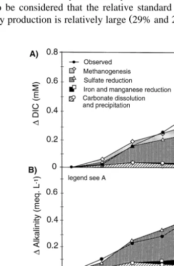
The expected and observed DIC production agreed well in the first half of the column ŽFig. 5A . In the second half, the observed DIC production was higher than expected.. However, the deviation was within the range of uncertainty. The expected alkalinity production corresponded well to the measured alkalinity production throughout the
Ž .
whole column Fig. 5B . The agreement between the expected and observed DIC and alkalinity production indicates that the postulated processes and the assumption that the oxidants were exclusively used for hydrocarbon mineralization are plausible. However, it has to be considered that the relative standard uncertainty of the observed DIC and
Ž .
alkalinity production is relatively large 29% and 24%, respectively . Furthermore, other
Ž . Ž .
Fig. 5. A Expected inorganic carbon production standard uncertainty"0.04 mM and observed inorganic
Ž . Ž . Ž
carbon production standard uncertainty"0.16 mM . B Expected alkalinity production standard uncertainty
y1. Ž y1. Ž .
"0.06 meq l and observed alkalinity production standard uncertainty"0.14 meq l . C Expected and
13 Ž . 13
observed d C of the dissolved inorganic carbon DIC . The standard uncertainty of the observed d C corresponds to the size of the marker.
processes than postulated in Table 3 may have occurred as well. For example, reduction
Ž . 2y
of FeOOH by S yII could also have lead to the formation of S O2 3 or polysulfides in
Ž . Ž .
addition to S 0 and FeS Dos Santos Afonso and Stumm, 1992; Peiffer et al., 1992 .
Ž .
The DIC balance Fig. 5A suggests that 67% of the DIC was produced by hydrocarbon mineralization coupled to SO2y reduction, 30% coupled to
methanogene-4
Ž . Ž .
sis, and 3% coupled to Fe III and Mn IV reduction. If CH4 is considered as end product of PHC mineralization in addition to DIC, hydrocarbon mineralization coupled to SO2y reduction and methanogenesis equally contributed to hydrocarbon
mineraliza-4
tion. DIC production by Ca- and Mg-carbonate dissolution corresponded approximately with DIC removal by the precipitation of FeCO . The main process producing alkalinity3
was SO2y reduction. 4
Ž . 2q Ž .
If S yII had been removed by precipitation with Fe Process 5b, Table 3 instead
Ž .
of reaction with FeOOH Process 5a, Table 3 , the expected alkalinity production would have been the same, since both processes are not tied to a net alkalinity production or consumption. The expected DIC production, however, would have been larger if one
Ž . 2q
assumes that the reduction of Fe III to produce the Fe necessary for the precipitation of the FeS was coupled to hydrocarbon mineralization. Hydrocarbon mineralization
Ž .
coupled to Fe III reduction would account for 11% instead of 3% of the expected DIC
Ž . Ž . 2y
production. If S yII had reacted with FeOOH to form Fe II and S O2 3 or
polysul-Ž 2y 2y. Ž . Ž .
fides S4 , S5 instead of FeS and S 0 , the contribution of Fe III reduction to Ž . hydrocarbon mineralization would have been smaller, since the produced Fe II would have partly originated from an abiotic process that is not coupled to hydrocarbon mineralization.
4.4. Stable carbon isotope balance
Since the d13C of DIC is dependent on the process responsible for its production, stable carbon isotope balances of the DIC can be used to verify the postulated processes. The d13C of the expected DIC was calculated based on two mass balance equations for 12 13
Ž . 13
C and C Hunkeler et al., 1997 and compared to the measured d C.
kq 1 k n
CDICsCDICq
Ý
DCDICŽ .
1n
kq 1 13 kq1 k 13 k n 13 n
C Pd C sC Pd C q
Ý
DC P d CŽ .
2DIC DIC DIC DIC DIC DIC
n
kq 1 k Ž .
where CDIC, CDIC mM is the expected DIC concentration at sampling ports k q 1 and
13 kq1 13 k Ž . 13
k, respectively; d CDIC, d CDIC ‰ is the expected d C at sampling ports k q 1
n Ž . Ž .
and k, respectively; DCDIC mM is the expected DIC production by process n Table 3 between sampling ports k and k q 1, which was quantified as discussed above; and
13 n Ž . 13 Ž .
d CDIC ‰ is the d C of DIC produced by process n Table 3 .
The calculation resulted in an increase of the d13C of the DIC by 2.2‰ between the
Ž .
sampling port at 2 cm and the column outlet Fig. 5C . Except for the shift between the Ž sampling port at 2 and 8 cm, the calculated and measured curves correspond well Fig.
. 13
5C . The increase of the d C was mainly caused by DIC production coupled to methanogenesis. The agreement between calculated and measured d13C in this study
turnover of oxidants and reduced species are plausible. A shift to a more positive d13C Ž
was also observed in field studies where methanogenic conditions were found Baedecker .
et al., 1993; Landmeyer et al., 1996 .
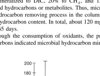
4.5. Carbon balance
A carbon balance was performed over the whole period of 65 days of column
Ž .
operation Fig. 6 , considering both mineralization of hydrocarbons to DIC and CH ,4
and elution of hydrocarbons and metabolites from the column. The total DIC production was calculated based on the observed DIC production, and was corrected for carbonate dissolution and precipitation. The elution of non-volatile metabolites from the column was assumed to be reflected in the measured DOC concentrations in the effluent. Since DOC concentrations were measured after vigorously bubbling the samples, it was assumed that DOC measurements did not reflect the elution of volatile aromatic hydrocarbons and volatile metabolites. Therefore, elution of these compounds was considered separately based on concentrations of dissolved hydrocarbons and metabo-lites measured in the pentane extract of the effluent.
The sum of carbon compounds in the effluent over the whole period of operation corresponded to the observed decrease of the hydrocarbon content in the aquifer material ŽFig. 6 . The carbon balance indicates that about 65% of the removed hydrocarbons. were mineralized to DIC, 20% to CH , and 15% were eluted from the column as4
unaltered hydrocarbons or metabolites. Thus, microbial mineralization was the predomi-nant hydrocarbon removing process in the column, accounting for 85% of the decrease of the hydrocarbon content. In total, about 120 mg C kgy1
dry weight were mineralized within 65 days.
Although the consumption of oxidants, the production of DIC and the removal of hydrocarbons indicated microbial hydrocarbon mineralization, no increase of the biomass
Fig. 6. Carbon balance over 65 days of column operation. DICmi ncorresponds to the total DIC production minus the DIC produced by carbonate dissolution.
in the column was observed. The increase of the biomass may have been smaller than the range of uncertainty of the detection method, since biomass yields of anaerobic
Ž
microbial cultures are usually low Edwards et al., 1992; Edwards and Grbic-Galic, .
1994 .
4.6. Degradation of selected compounds
Ž Since n-alkanes were removed from the aquifer material in contrast to i-alkanes Fig.
.
3A,B, Table 1 , it can be concluded that n-alkanes were degraded and possibly mineralized. Their transformation to dissolved metabolites is unlikely because the elution of DOC was 6 times smaller than the decrease of the n-alkane content in the aquifer material. Assuming that the alkanes were completely mineralized, half of the consumption of oxidants and production of reduced species can be attributed to the mineralization of n-alkanes.
In Fig. 4B,C,D, the ratios of the actual to the initial concentration of various
mono-Ž .
and di-aromatic compounds denoted as relative concentrations are shown. The relative concentration of ethylbenzene, o-xylene and m-xylene decreased to about 0.7 within 65
Ž .
days of column operation Fig. 4B . The relative concentration of toluene and p-xylene decreased to less than 0.1 within 24 days. Since toluene and p-xylene have similar
Ž .
physical–chemical properties Table 2 as ethylbenzene, o-xylene, and m-xylene, a similar decrease of the relative concentration would be expected if all compounds were only removed by elution from the column. The much faster decrease of the relative concentration of toluene and p-xylene compared to the other compounds suggests that toluene and p-xylene were removed by microbial degradation in addition to elution from the column. The relative concentrations of the propylbenzenes, ethylbenzenes,
trimethyl-Ž .
and tetramethylbenzenes, given in Table 2 Nos. 6–13 , remained constant during the entire operation period. In Fig. 4C, the relative concentrations are illustrated for
n-propylbenzene, 2-ethyltoluene, and 1,2,4-trimethylbenzene. The constant relative
con-centrations indicate that no significant loss of these compounds during the period of the experiment either by elution or by biodegradation. The relative concentrations of naphthalene decreased to about 0.6 while the ratio of 1- and 2-methylnaphthalene
Ž .
remained constant Fig. 4D , suggesting that biodegradation of naphthalene probably did occur.
Thus, the analysis of hydrocarbon concentrations in the aquifer material and the effluent of the column indicates that, of the identified compounds, n-alkanes, toluene,
p-xylene and naphthalene were degraded with lag phases of less than 65 days at
observable rates. Biodegradation of these compounds in the absence of O and NOy
2 3
Ž was also observed in various microbial cultures, in microcosms and field studies Lovley and Lonergan, 1990; Aeckersberg et al., 1991; Edwards et al., 1992; Edwards and Grbic-Galic, 1994; Thierrin et al., 1995; Ball and Reinhard, 1996; Beller et al., 1996;
. Ž
Coates et al., 1996 . The elution of other compounds at constant concentrations e.g.,
. Ž .
trimethylbenzene or at constant ratios e.g., ethylbenzene to o-xylene and m-xylene in our study does not mean that these compounds are not biodegradable in the absence of O and NOy
. To degrade these compounds, a longer incubation time may be required.
2 3
In addition, the presence of easily degradable compounds may inhibit the degradation of Ž other compounds. A sequential degradation of monoaromatic compounds toluene,
. 2y
p-xylene and o-xylene under SO4 reducing conditions was observed in a microcosm
Ž .
study by Edwards et al. 1992 . In their study, toluene was degraded first followed by
p-xylene and finally o-xylene. 4.7. Implications for bioremediation
This study demonstrates that in the absence of O and NOy
, hydrocarbon
mineraliza-2 3
tion coupled to SO2y reduction and methanogenesis can substantially contribute to the 4
removal of hydrocarbons from contaminated aquifer material. Hydrocarbon
mineraliza-Ž . Ž .
tion coupled to Fe III and Mn IV reduction was of minor importance in our study. In field cases, a larger percentage of the hydrocarbon mineralization may be coupled to
Ž . Ž .
Fe III and Mn IV reduction due to the longer residence time of the water in the contaminated zone. DIC, alkalinity, and stable carbon isotope balances were shown to be a useful tool to verify hydrocarbon mineralization.
Ž
In the columns, selected aromatic compounds of toxicological concern e.g., toluene, .
p-xylene and naphthalene and n-alkanes were degraded. However, some other
com-pounds such as ethylbenzene, m-xylene, o-xylene and trimethylbenzenes were not degraded at significant rates, but eluted from the column at a constant concentration over the entire period of the experiment. If a similar degradation pattern is observed in field cases, these compounds may pollute the groundwater over a longer period of time. However, the more recalcitrant compounds may be degraded as well, once the more degradable compounds are mineralized, or they may be degraded in zones of the aquifers where aerobic or denitrifying conditions are re-established due to mixing of
Ž .
polluted with unpolluted groundwater Eganhouse et al., 1996 .
Acknowledgements
We thank J. McKenzie, S. Bernasconi and J. Teranes for providing the facilities for isotope analysis and for helpful discussions; A. Haner and T. Bregnard for the assistance
¨
in hydrocarbon analysis; and G.T. Townsend and two referees for reviewing the Ž manuscript. The work was supported by the Swiss National Science Foundation Priority
. Programme Environment .
References
Aeckersberg, F., Bak, F., Widdel, F., 1991. Anaerobic oxidation of saturated hydrocarbons to CO by a new2
type of sulfate-reducing bacterium. Arch. Microbiol. 156, 5–14.
Ž .
APHA American Public Health Association , 1989. Standard methods for the examination of water and wastewater, Am. Public Health Association, Washington, DC, 981 pp.
Baedecker, M.J., Cozzarelli, I.M., Eganhouse, R.P., Siegel, D.I., Bennett, P.C., 1993. Crude oil in a shallow sand and gravel aquifer: III. Biogeochemical reactions and mass balance modeling in anoxic groundwater. Appl. Geochem. 8, 569–586.
Balkwill, D.L., Leach, F.R., Wilson, J.T., McNabb, J.F., White, D.C., 1988. Equivalence of microbial biomass measures based on membrane lipid and cell wall components, adenosine triphosphate, and direct counts in subsurface aquifer sediments. Microb. Ecol. 16, 73–84.
Ball, H.A., Reinhard, M., 1996. Monoaromatic hydrocarbon transformation under anaerobic conditions at Seal Beach, California: Laboratory studies. Environ. Toxicol. Chem. 15, 114–122.
Battermann, G., 1983. A large scale experiment on in situ biodegradation of hydrocarbons in the subsurface. In: Ground Water in Water Resources Planning, Vol. II, IASA Publication 142. Int. Association of Hydrological Sci., London, pp. 983–987.
Beller, H.R., Spormann, A.M., Sharma, P.K., Cole, J.R., Martin, R., 1996. Isolation and characterization of a novel toluene-degrading sulfate-reducting bacterium. Appl. Environ. Microbiol. 62, 1188–1196. Borden, R.C., Gomez, C.A., Becker, M.T., 1995. Geochemical indicators of intrinsic bioremediation. Ground
Water 33, 180–189.
Ž .
Bouwer, E.J., 1992. Bioremediation of organic contaminants in the subsurface. In: Mitchell, R. Ed. , Environ. Microbiol. Wiley, New York, pp. 287–318.
Bregnard, T.P.-A., Hohener, P., Haner, A., Zeyer, J., 1996. Degradation of weathered diesel fuel by¨ ¨
microorganisms from a contaminated aquifer in aerobic and anaerobic microcosms. Environ. Toxicol. Chem. 15, 299–307.
Carothers, W.W., Adami, L.H., Rosenbauer, R.J., 1988. Experimental oxygen isotope fractionation between siderite-water and phosphoric acid liberated CO -siderite. Geochim. Cosmochim. Acta 52, 2445–2450.2
Coates, J.D., Anderson, R.T., Lovley, D.R., 1996. Oxidation of polycyclic aromatic hydrocarbons under sulfate-reducing conditions. Appl. Environ. Microbiol. 62, 1099–1101.
Coplen, T.B., 1996. New guideline for reporting stable hydrogen, carbon, and oxygen isotope-ratio data. Geochim. Cosmochim. Acta 60, 3359–3360.
Ž .Ž .
Dos Santos Afonso, M., Stumm, W., 1992. The reductive dissolution of iron III hydr oxides by hydrogen sulfide. Langmuir 8, 1671–1675.
Eastcott, L., Shiu, W.Y., Mackay, D., 1988. Environmentally relevant physical-chemical properties of hydrocarbons: A review of data and development of simple correlations. Oil and Chemical Pollution 4, 191–216.
Edwards, E.A., Wills, L.E., Reinhard, M., Grbic-Galic, D., 1992. Anaerobic degradation of toluene and xylene by aquifer microorganisms under sulphate-reducing conditions. Appl. Environ. Microbiol. 58, 794–800. Edwards, E.A., Grbic-Galic, D., 1994. Anaerobic degradation of toluene and o-xylene by a methanogenic
consortium. Appl. Environ. Microbiol. 60, 313–322.
Eganhouse, R.P., Dorsey, T.F., Phinney, C.S., Westcott, A.M., 1996. Processes affecting the fate of monoaromatic hydrocarbons in an aquifer contaminated by crude oil. Environ. Sci. Technol. 30, 3304–3312. Essaid, H.I., Bekins, B.A., Godsy, M.E., Ean, W., 1995. Simulation of aerobic and anaerobic biodegradation
processes at a crude oil spill site. Water Resour. Res. 31, 3309–3327.
Furrer, G., von Gunten, U., Zobrist, J., 1996. Steady-state modelling of biogeochemical processes in columns with aquifer material: I. Speciation and mass balances. Chem. Geol. 133, 15–28.
Grossman, E.L., Coffman, K., Fritz, S.J., Wada, H., 1989. Bacterial production of methane and its influence on groundwater chemistry in east-central Texas aquifers. Geology 17, 495–499.
Grossman, E.L., 1997. Stable carbon isotopes as indicators of microbial activity in aquifers. In: Hurst, C.J.
ŽEd. , Manual of Environ. Microbiol., Am. Soc. for Microbiol., Washington, DC, pp. 565–576..
Hahn, D., Ammann, R.I., Ludwig, W., Akkermans, A.D.L., Schleifer, K.H., 1992. Detection of microorgan-isms in soil after in situ hybridization with rRNA-targeted, fluorescently labelled oligonucleotides. J. Gen. Microbiol. 138, 879–887.
Haner, A., Hohener, P., Zeyer, J., 1995. Degradation of p-xylene by a denitrifying enrichment culture. Appl.¨ ¨
Environ. Microbiol. 61, 3185–3188.
Herczeg, A.L., Richardson, S.B., Dillon, P.J., 1991. Importance of methanogenesis for organic carbon mineralisation in groundwater contaminated by liquid effluent, South Australia. Appl. Geochem. 6, 533–542.
Ž . Ž .
Heron, G., Crouzet, C., Bourg, A.C.M., Christensen, T.H., 1994. Speciation of Fe II and Fe III in contaminated aquifer sediments using chemical extraction techniques. Environ. Sci. Technol. 28, 1698– 1705.
Hess, A., Hohener, P., Hunkeler, D., Zeyer, J., 1996. Bioremediation of a diesel fuel contaminated aquifer:¨
simulation studies in laboratory aquifer columns. J. Contam. Hydrol. 23, 329–345.
Holliger, C., Zehnder, A.J.B., 1996. Anaerobic biodegradation of hydrocarbons. Curr. Opin. Biotechnol. 7, 326–330.
Hunkeler, D., Hohener, P., Haner, A., Bregnard, T.P.-A., Zeyer, J., 1995. Quantification of hydrocarbon¨ ¨
Ž .
J. Eds. , Groundwater Quality: Remediation and Protection. IAHS Publication No. 225, IAHS Press, Wallingford, Oxfordshire, pp. 421–430.
Hunkeler, D., Hohener, P., Bernasconi, S., Zeyer, J., 1997. In situ bioremediation of petroleum hydrocarbon¨
contaminated aquifer: assessment of mineralization based on alkalinity, inorganic carbon and stable carbon isotope balances. J. Contam. Hydrol., submitted.
Hutchins, S.R., Downs, W.C., Wilson, J.T., Smith, G.B., Kovacs, D.A., Fine, D.D., Douglass, R.H., Hendrix, D.J., 1991. Effect of nitrate addition on biorestoration of fuel-contaminated aquifer: field demonstration. Ground Water 29, 571–580.
International Organization for Standardization, 1993. Guide to the expression of uncertainty in measurement, Int. Org. for Standardization, Geneva, 101 pp.
Landmeyer, J.E., Vroblesky, D.A., Chapelle, F.H., 1996. Stable carbon isotope evidence of biodegradation zonation in a shallow jet-fuel contaminated aquifer. Environ. Sci. Technol. 30, 1120–1128.
Lovley, D.R., Lonergan, D.J., 1990. Anaerobic oxidation of toluene, phenol, and p-cresol by the dissimilatory iron-reducing organism GS-15. Appl. Environ. Microbiol. 56, 1858–1864.
Ž .
Lovley, D.R., Phillips, E.J.P., Lonergan, D.J., 1991. Enzymatic versus nonenzymatic mechanisms for Fe III reduction in aquatic sediments. Environ. Sci. Technol. 25, 1062–1067.
Madsen, E.L., 1991. Determining in situ biodegradation: facts and challenges. Environ. Sci. Technol. 25, 1663–1673.
Matsunaga, T., Karametaxas, G., von Gunten, H.R., Lichtner, P.C., 1993. Redox chemistry of iron and manganese minerals in river-recharged aquifers: a model interpretation of a column experiment. Geochim. Cosmochim. Acta 57, 1691–1704.
Millner, G.C., Nye, A.C., Jamer, R.C., 1992. Human health based soil cleanup guidelines for diesel fuel No. 2.
Ž .
In: Kostecki, P.T., Calabrese, E.J. Eds. , Contaminated Soils: Diesel Fuel Contamination. Lewis Publish-ers, Chelsea, MI, pp. 165–216.
Peiffer, S., Dos Santos Afonso, M., Wehrli, B., Gachter, R., 1992. Kinetic and mechanism of reaction of H S¨ 2
with lepidocrocite. Environ. Sci. Technol. 26, 2408–2413.
Ž . Ž .
Stone, A.T., Morgan, J.J., 1984. Reduction of manganese III and manganese IV oxides by organics: 2. Survey of the reactivity of organics. Environ. Sci. Technol. 18, 617–624.
Stumm, W., Morgan, J.J., 1996. Aquatic Chemistry. Wiley, New York, 1022 pp.
Thierrin, J., Davis, G.B., Barber, C., 1995. A ground-water tracer test with deuterated compounds for monitoring in situ biodegradation and retardation of aromatic hydrocarbons. Ground Water 33, 469–476.
Ž .
Thomas, J.M., Ward, C.H., 1994. Introduced organisms for subsurface bioremediation. In: Norris, R.D. Ed. , Handbook of Bioremediation. CRC Press, Boca Raton, FL, pp. 227–244.
Thorstenson, D.C., Plummer, L.N., 1977. Equilibrium criteria for tow component solids reacting with fixed composition in an aqueous phase—example: the magnesium calcites. Am. J. Sci. 277, 1203–1233. Toride, N., Leij, F.J., van Genuchten, M.T., 1995. The CXTFIT code for estimating transport parameters from
laboratory or field tracer experiments. US Salinity Laboratory, Agricultural Res. Service, Riverside, CA, August 1995, Res. Report No. 137.
US Environmental Protection Agency, 1989. Test methods for evaluating solid waste Physicalrchemical methods. US Department of Commerce, National Technical Information Service, Washington, DC. US National Research Council, 1993. In situ bioremediation: when does it work? Natl. Academy Press,
Washington, DC, 207 pp.
Von Gunten, U., Zobrist, J., 1993. Biogeochemical changes in groundwater-infiltration systems: column studies. Geochim. Cosmochim. Acta 57, 3895–3906.
Westall, J.C., 1986. A chemical equilibrium program in basic. Department of Chemistry, Oregon State Univ., Corvallis, OR.
Whiticar, M.J., Faber, E., Schoell, M., 1986. Biogenic methane formation in marine and freshwater environments: CO2 reduction vs. acetate fermentation—isotopic evidence. Geochim. Cosmochim. Acta 50, 693–709.
Ž .
Zehnder, A.J.B., Zinder, S.H., 1980. The sulfur cycle. In: Hutzinger, O. Ed. , The Handbook of Environmen-tal Chemistry, Vol. 1rPart A, Springer, Berlin, pp. 105–145.
Zeyer, J., Kuhn, E.P., Schwarzenbach, R.P., 1986. Rapid microbial mineralization of toluene and 1,3-dimeth-ylbenzene in the absence of molecular oxygen. Appl. Environ. Microbiol. 52, 944–947.