Aerodynamic design of an aspirated counter-rotating compressor

Aerodynamic Design of an Aspirated

Counter-Rotating Compressor

by

Jody Kirchner

B.A.Sc (Mechanical Eng), University of British Columbia (2000)

Submitted to the Department of Aeronautics and Astronautics

in partial fulfillment of the requirements for the degree of

Master of Science

at the

MASSACHUSETTS INSTITUTE OF TECHNOLOGY

June 2002

@

Massachusetts Institute of Technology 2002. All rights reserved.

A uthor ...

...

Dep$rtrent of Aeronautics and Astronautics

May 1, 2002

Certified by...

Jack L. Kerrebrock

Professor Emeritus of Aeronautics and Astronautics

Thesis Supervisor

Accepted by...

...

Wallace E. Vander Velde

Professor of Aeronautics and Astronautics

Chair, Committee on Graduate Students

MASSACHUSETTS iNSTITUTE OF TECHNOLOGY

AERO

Aerodynamic Design of an Aspirated Counter-Rotating

Compressor

by

Jody Kirchner

Submitted to the Department of Aeronautics and Astronautics on May 1, 2002, in partial fulfillment of the

requirements for the degree of Master of Science

Abstract

A primary goal in compressor design for jet engines is the reduction of size and weight. This can be achieved by increasing the work output per stage, thereby reducing the required number of stages. In this thesis, the aerodynamic design of a high speed compressor that produces a pressure ratio of 9.1:1 in only two stages (rather than the typical six or seven) is presented. This is accomplished by employing blade aspiration in conjunction with rotor counter-rotation. Aspiration has been shown to make feasible significantly increased blade loading and counter-rotation provides a means of taking full advantage of this potential throughout a multistage compressor.

The aspirated counter-rotating compressor was designed using a one-dimensional stage analysis program coupled with an axisymmetric throughflow code and a quasi-three-dimensional cascade code for blade design. The design of each stage focussed on maximising pressure ratio within diffusion factor and relative inlet Mach number (i.e. shock loss) constraints. The exit angle of the first stator was optimised to maximise the pressure ratio of the counter-rotating (second) rotor. The blade design code MISES allowed for each feature of the blade sections, including aspiration, to be precisely designed for the predicted conditions. To improve the process of designing blades with MISES, extensive analysis of previously designed high-speed aspirated blades was performed to identify the relationships between various blade features. Thesis Supervisor: Jack L. Kerrebrock

Acknowledgments

I would like to thank my advisor Professor Jack Kerrebrock for suggesting this project, providing guidance while giving me space to figure things out on my own, and, perhaps most importantly, keeping me excited about the project along the way.

I would also like to thank Ali Merchant for providing supervision and for putting up with my struggles with all the CFD programs. Also, thanks for writing an excellent PhD thesis which was an invaluable reference for this work. Thanks to Brian Schuler for teaching me how to use MISES and for providing assistance along the way.

Finally, a very special thanks to all the friends I have made at MIT who have helped make this a great experience.

Contents

1 Introduction

1.1 _{Motivation and Background . . . .}

1.2 O bjectives . . . . 1.3 O utline. . . . . 2 Compressor Theory 2.1 Stage A nalysis . . . . 2.2 Dimensionless Parameters . . . . 2.3 Losses ... ... 2.3.1 _{V iscous Losses . . . .} 2.3.2 _{Shock Losses . . . .} 2.4 A spiration . . . . 3 Design Methodology and 0

3.1 Design Process . . . .

3.2 Goals and Constraints . .

4 Stage and Flowpath Design

4.1 Stage Analysis . . . . 4.1.1 Work Distribution 4.1.2 Interstage Swirl . . 4.1.3 Geometry . . . . . 4.2 Flowpath Generation . . . bjectives . . . . . . . . 13 13 17 17 19 19 21 22 23 24 25 29 29 31 33 33 34 34 36 37

4.3 Throughflow Analysis . . . . 38 4.3.1 Code Description . . . . 39 4.3.2 Results . . . . 40 4.4 Design Summary . . . . 41 5 Blade Design 45 5.1 Code Description . . . . 45 5.2 Design Process . . . . 47 5.3 Blade Features . . . . 51 5.3.1 Incidence . . . . 52 5.3.2 Camber Distribution . . . . 54 5.3.3 Thickness Distribution . . . . 56 5.3.4 Leading Edge . . . . 58 5.3.5 Trailing Edge . . . . 59 5.3.6 Aspiration . . . . 60

5.4 Final Blade Designs. . . . . 61

5.4.1 Stage 1. . . . . 61

5.4.2 Stage 2. . . . . 67

5.4.3 Summary . . . . 72

6 Conclusion 75 6.1 Compressor Design Summary . . . . 75

6.2 Concluding Remarks on Design Process . . . . 76

6.3 Future W ork . . . . 77

List of Figures

1-1 Work output of counter-rotating relative to conventional compressor 1-2 Conventional modern engine and conceptual engine with aspirated

counter-rotating compressor (adapted from Reference [8]) . . . .

2-1 Compressor stage nomenclature . . . .

2-2 Correlation of diffusion factor and loss parameter .

2-3 Variation of entropy rise due to shock loss with inlet

2-4 Suction slot (adapted from Reference [18]) . . . . .

2-5 Effect of aspiration on a blade boundary layer [18] .

3-1 Compressor design process . . . .

4-1 Variation of rotor 2 diffusion factor with inlet swirl 4-2 Stator 1 exit angle distribution . . . . 4-3 Flowpath and blades . . . . 4-4 Throughflow pressure contours . . . . 4-5 Velocity triangles . . . . 5-1 5-2 5-3 5-4 5-5 5-6 5-7 Mach number 15 16 20 24 26 . . . . 27 . . . . 27 . . . . 30 . . . . 35 . . . . 36 . . . . 38 . . . . 41 . . . . 42

Blade section design flowchart . . . . Blade pressure distribution design templates . . . . Correction of blade surface bump . . . . Impact of blade surface bump on inviscid pressure distribution Blade section parameters . . . . Stagger angle versus turning angle . . . . Maximum camber versus turning angle . . . . . . . . 48 . . . . 49 . . . . 50 50 51 54 55

5-8 Typical rotor camber di 5-9 Maximum thickness ver 5-10 Leading edge radius ver 5-11 Diverging trailing edge 5-12 5-13 5-14 5-15 5-16 5-17 5-18 5-19 5-20 5-21 5-22 5-23 5-24 5-25 A-i A-2 A-3 A-4 A-5 A-6 A-7 A-8 hape hap stributions . . . . .

sus inlet Mach number sus inlet Mach number

paraete... ..pramte... ... parameter . . . . ... e parameter . . . . ... ... . . . . . . . . Rotor 1 hub . ... Rotor 1 50% span . Rotor 1 50% span s Rotor 1 tip . . . . Stator 1 hub . ... Stator 1 50% span Stator 1 50% span s Stator 1 tip . . . . Rotor 2 hub . ... Rotor 2 50% span . Rotor 2 tip . . . . Stator 2 hub . ... Stator 2 50% span Stator 2 tip . . . . Rotor 1 25% Span . Rotor 1 75% Span . Stator 1 25% Span Stator 1 75% Span Rotor 2 25% Span. Rotor 2 75% Span. Stator 2 25% Span Stator 2 75% Span 56 58 59 60 62 63 63 64 65 66 66 67 68 69 70 71 72 72 83 84 84 85 85 86 86 87

List of Tables

3.1 Design goals and constraints . . . . 31

4.1 Stage design results . . . . 43

Chapter 1

Introduction

1.1

Motivation and Background

A driving force in compressor design is the desire to achieve a high pressure ratio and efficiency while maintaining or decreasing the size (particularly length) and weight of the compressor. It is also beneficial to reduce the number of parts, especially blades which are expensive to produce and maintain. To this end it is necessary to develop means of improving the performance of individual compressor stages so that fewer stages are required for a given application.

The pressure ratio attainable in a compressor stage has traditionally been limited by viscous effects on the blades, in particular flow separation. However, recent work by Kerrebrock and others has shown that removing a portion of the boundary layer fluid from the blade surface through aspiration can delay separation and allow for significantly increased blade loading (see for example [11], [12]). This in turn reduces the number of stages required to obtain the desired compressor pressure ratio. A low-speed compressor stage employing aspiration has been built and tested success-fully [18, 21] and a high-speed stage has been designed and is under construction for testing [18]. With aspiration shown to be viable way of raising the loading limits of blades, it is an opportune time to consider means of taking advantage of the ability to do more work with each stage.

stationary blade row, or stator. The rotor does work on the fluid given by

WR = w(r 2v2 - riV) (1.1)

where w is the angular velocity and rv is the angular momentum per unit mass (also called swirl) at the inlet (1) and exit (2). The stator converts some fraction of the rotor work into a static pressure rise. Equation 1.1 shows that there are two ways to increase the work of a stage: increase the tip speed and increase the change in swirl or turning. However, tip speed in modern compressors is limited by structural constraints, so increased turning must be considered as a means to obtain any increase in work.

There is a wide range of design options to choose from in selecting the swirl at the inlet to the rotor, riv1, but in modern high-work compressors the stators typically remove all of the swirl from the upstream rotors, so that the flow entering each rotor is axial (rivi = 0). Even with advances in blade design, there is a limit on how far the rotor can turn the flow from the axial direction and, therefore, how much work it can do on the flow. However, if the flow entering the rotor has swirl against the direction of rotation (riv < 0), for the same rotor exit angle the amount of work is increased. This can be achieved throughout a multistage compressor by reducing the turning of the stators (or removing the stators altogether) and alternating the direction of rotation of the spools. This is termed counter-rotation.

Figure 1-1 shows the ratio of the ideal work output of a simple two-stage counter-rotating compressor to that of a conventional two-stage compressor given by

Wcounter _ wr(vc - Vb)counter - 1 +-tan

WeO wr(ve - Vb)cO 2

where a is the exit angle of the first stator for the counter-rotating configuration. Geometrically, the configurations are identical except for the exit angle of the first stator which is zero for the conventional configuration and varies for the counter-rotating configuration. This simple analysis shows that a significant increase in work is possible with counter-rotation.

A more extensive assessment of the performance improvement possible for a single compressor stage with inlet counter-swirl was made by Law and Wennstrom [14].

1.5

1.45-

-~1.4-1 Rotor 1 Stator 1: Rotor 2 Stator 2

variable . 1.35- exit angle

- All swirl left in flow

-2 1.3 no stator 1.25- 1.2-0 1.15-0 o 1.1 1.05-1 0 0.1 0.2 0.3 0.4 0.5 0.6 0.7 0.8 0.9 1

Fraction of swirl remaining after Stator 1

Figure 1-1: Work output of counter-rotating relative to conventional compressor

They designed and tested a stage with counter-swirl imparted by inlet guide vanes. With a tip speed of 1500ft/sec the rotor successfully achieved a pressure ratio of 2.42 at a peak isentropic efficiency of 91.6%. The stage pressure ratio and isentropic efficiency were 2.30 and 85.8% respectively.

The use of counter-rotation in previous compressor designs has not resulted in such a considerable improvement. Since the feasible increase in blade loading has been restricted by viscous effects, a large number of stages have still been required. However, mechanical limitations make possible the application of counter-rotation between only a few stages, so the overall impact on performance has been low. How-ever, in a compressor with few stages (two or three), such as would be feasible with aspirated blades, the benefits of counter-rotation can be captured by each stage with-out an unrealistically large number of spools. Therefore there is an opportunity for significant performance improvement if aspiration and counter-rotation are utilised

together.

Preliminary work was done at MIT by Freedman to determine the best config-uration for an aspirated counter-rotating compressor and for the engine in which

it would operate [9]. Several compressor configurations involving different

combina-tions of rotors and stators were investigated, but it was concluded that a conventional rotor-stator configuration was optimal. Attempts to maximise the residual swirl and minimise the compressor length by removing the stators resulted in unacceptably high Mach numbers and losses in the rotors. The compressor and engine configuration that was developed previously is shown schematically in Figure 1-2 along with a conven-tional modern engine with the same pressure ratio for comparison. The decrease in the length of the engine made possible by increasing the work output per stage via counter-rotation and aspiration is significant.

Conventional

Aspirated Counter-rotating

Figure 1-2: Conventional modern engine and conceptual engine with aspirated

1.2

Objectives

The purpose of this work was to continue with the development of the multi-stage aspirated counter-rotating compressor discussed in Section 1.1. More specifically, the primary goal was to produce a detailed aerodynamic design of a two-stage compressor to be tested in the Blowdown Compressor facility at MIT. These tests will be used to assess the validity of the aspirated counter-rotating concept for use in practical applications.

Although other applications are possible, it is presently thought that an aspirated counter-rotating compressor would be ideal for use as a core compressor in a long range supersonic cruise aircraft. This is mainly because such aircraft are especially sensitive to weight. This foreseen application provided the basis for many of the parameters of the current design.

1.3

Outline

The body of this thesis details the steps and results of the compressor design. Chapter 2 provides a theoretical background for the work, including the important parameters and equations for the stage analysis and evaluation of losses and aspiration. The steps of the design process as well as the goals and constraints are presented in Chapter 3. Chapter 4 discusses the design of the compressor stages and the flowpath including the work distribution and geometry choices. The results of a computational throughflow analysis are also presented in this chapter. Chapter 5 describes the design of the blade sections using a quasi-three-dimensional turbomachinery cascade code and presents the final blade designs. Finally, Chapter 6 provides some conclusions, including a summary of the compressor design as well as a discussion of future work.

Chapter 2

Compressor Theory

2.1

Stage Analysis

In a one-dimensional compressor stage analysis, the flow through a blade row (rotor and stator) is described by the changes in velocity components as shown in Figure 2-1. The components shown as solid vectors represent absolute velocities and those shown as dotted vectors represent velocities relative to the rotating frame of reference of the rotor. The conditions at the stage inlet (denoted with the subscript 1) are known either from the compressor inlet conditions (for the first stage) or the upstream stage exit conditions (for subsequent stages). To simplify the analysis, it is often assumed that the axial velocity, w, is constant, although in reality it will fluctuate across the blade rows.

The change in tangential velocity, v, across the rotor can be related to the stag-nation temperature, T, rise by the Euler equation

C,(T2- Tti) = w(r2v2 - riv1) (2.1)

where w is the rotational speed, r is the radius, and c, is the specific heat at constant pressure. In the design problem considered here, the stagnation temperature change is fixed by the desired pressure ratio and the required tangential velocity change must be found. The pressure ratio

=

-(2.2) Pt1

ROTOR STATOR v V2 V3 P3i Vcr V2~ W r w2 v or W3 owr j3/ _V2

Figure 2-1: Compressor stage nomenclature and temperature ratio

T - - (2.3)

T

are related by the efficiency of the stage, TI, which is the ratio of the ideal work of the blade row to the actual work required to give the desired pressure ratio. The efficiency is affected by entropy losses due to viscous shear forces, shocks, etc. In a simplified stage analysis, a value of efficiency is assumed at the start so that the temperature ratio can be found from

T = 1 + (2.4)

where -y is the ratio of specific heats.

With the required tangential velocity downstream of the rotor known from the Euler equation, the other velocity components at this position can be found from geometry. The relations are

V2 = W - V2 (2.5)

V2 /= w2 +v 22 , V2'= W2+4 , (2.6)

V2V2 V2+ V

02 = arctan , and

#'2

).

The primed values are relative to the rotor frame of reference.

The flow through the stator involves only diffusion without energy addition and generally the exit angle of the stator is a flexible design parameter. It is chosen based

on the inlet flow desired for the downstream component, within the aerodynamic constraints of the blade (for example, the separation characteristics). Once the stator exit angle is chosen, the velocity components at that position can be found from

V3 = wtan/33 , and (2.8)

V = w2 +v 32 . (2.9)

Generally, it is useful to represent the velocities through the compressor as Mach numbers given by

M=- . (2.10)

a The quantity a is the local speed of sound

V2

a = RT = yR (T - 2p(2.11)

where R is the specific gas constant, and T is the static temperature.

For a counter-rotating compressor stage, the analysis is the same as that for a conventional stage except that the tip speed used in the Euler equation is negative. When determining the velocity components geometrically, care must be taken to use tangent and sine functions rather than cosine so that the negative relative velocities

are preserved.

2.2

Dimensionless Parameters

From the quantities obtained in the stage analysis, several useful dimensionless pa-rameters can be defined, in addition to the pressure and temperature ratios. These dimensionless parameters are useful in summarising a compressor design since val-ues for different compressors can be compared more directly than can dimensional parameters.

The work done across the stage, cAT, and the rotor speed, wr, are combined to give the stage loading coefficient which is a measure of the fraction of blade energy transferred to the fluid

w=)2 _{. (2.12)}

The axial velocity, w, and the rotor speed are combined to give the flow coefficient w

=_ .(2.13)

The absolute value of the rotational speed is used here so that the flow coefficient will be positive for the counter-rotating rotor. The distribution of loading in the stage is represented by the degree of reaction which is the ratio of the static enthalpy, cT, rise in the rotor to that in the stage

RC = T T (2.14)

T3 - T1

The fractional change in axial velocity through a blade row is termed the axial velocity ratio

AVR = . (2.15)

W1

This value is important to blade boundary layer behaviour which depends heavily on whether the flow is accelerating (AVR > 1) or decelerating (AVR < 1). In the stage analysis described in Section 2.1, the axial velocity ratio will be equal to one (since axial velocity is assumed constant), but this will not in general be the case. For flow in which large density changes occur, such as in high-speed compressors, a more useful parameter is the axial velocity density ratio

AVDR - P (2.16)

p1w1

which represents the streamtube contraction or expansion through the blade row.

2.3

Losses

In low-speed compressors the most significant source of loss is viscous shear on the blades. However, for high-speed compressors, such as that considered here, shock losses can be up to seven or eight times larger than viscous losses (as seen with the aspirated blades designed by Merchant [18]). Therefore, an accurate model for both types of loss is important. More minor sources of loss such as tip leakage losses and possible shroud losses are not considered here.

To avoid results that are dependant on the frame of reference (moving for the rotor and stationary for the stator), the losses are presented in terms of the resulting entropy increase in the flow, As [10]. The entropy rises due to each component of loss for the rotor and stator can be added to give the total entropy increase for the stage. The entropy rise and temperature ratio of the stage give the adiabatic efficiency

res* 0 /cP - 1

T-=l .(2.17)

2.3.1

Viscous Losses

Viscous losses in cascades are represented by a non-dimensional pressure loss coeffi-cient

A = . _(2.18)

Pt - P1

Analysis of cascade data by Lieblein [15] lead to a correlation between the loss coeffi-cient and the now widely used diffusion factor which is a measure of the deceleration

of the flow through the blade passages. The diffusion factor is given by

D = 1 V2 + |v2 - v1 (2.19)

V1 2-Vi

where the subscript 1 represents relative inlet flow and the subscript 2 represents relative exit flow. The solidity of the cascade, o, is the ratio of the chord length to the blade spacing. Figure 2-2 shows the Lieblein correlation between the loss parameter which is a function of the loss coefficient and the diffusion factor

W 2cos c f (D) . _(2.20)

cs1

2o-For low diffusion factors (below about 0.45) the viscous loss is almost constant, but above this value the loss increases rapidly due to boundary layer separation. For this reason, conventional blades are generally limited to diffusion factors well below 0.5.

Adding aspiration to blades reduces the boundary layer thickness. Therefore, it is possible to go to higher diffusion factors before approaching separation and incurring a rapid increase in loss. Schuler [21] presents a correlation between the diffusion factor and the loss parameter for aspirated blades, similar to Lieblein's correlation for conventional blades. This is also shown in Figure 2-2.

0 0.1 0.2 0.3 0.4 0.5 0.6 Diffusion factor

0.7 0.8 0.9 1

Figure 2-2: Correlation of diffusion factor and loss parameter Once the diffusion factor for a blade row has been determined from using Equation 2.19, the loss coefficient can be found from Figure 2-2 tionships derived from these curves (for example, see Reference [21]). rise corresponding to the loss coefficient is

the velocities or from rela-The entropy

a~sviscous

where the stagnation pressure, P'2, is relative to the frame of reference moving with

the blade row.

2.3.2

Shock Losses

Although shock losses have a significant impact on the performance of supersonic compressors, the models available are not as well established as those for viscous losses. Kerrebrock [10] suggests that the shock loss for a blade row be estimated as the average of the loss due to a normal shock at the relative inlet Mach number

0.06 0.05 0.04 0.03 ED a 0--J Conventional - - Aspirated -/ 0.02 0.01 0 1.1 '

and the loss due to a normal shock at the suction surface impingement location Mach number. Experimental data has shown that the actual shock losses in rotors are lower than predicted by this method, so it provides a conservative estimate.

The blade relative Mach number will be known from the stage analysis, but the shock impingement Mach number must be estimated since the position of the shock will not generally be known at this point in the design. Based on aspirated blades designed by Merchant, Schuler [21] presents an equation to estimate the shock im-pingement Mach number,

Mimp = 1.225Mre. (2.22)

With the Mach numbers known, the corresponding entropy rise through the shock is

27) 2 2+ (7y - 1)M 2'\ 27) 2"

/.XSshock cpn I + (M2 - 1) -Rln I + (M2 _ 1)

7+ 1(7y + 1) M2 7+ 1

(2.23) The average of the entropy rises at the two Mach numbers provides the entropy rise for the blade row.

The relationship between blade relative inlet Mach number and entropy rise due to shock loss (normalised by c,) is plotted in Figure 2-3. From the plot it is evident that above a relative inlet Mach number of about 1.5, losses begin to rise quickly above the low values seen at transonic Mach numbers. This is a useful guideline for supersonic compressor stage design.

2.4

Aspiration

Aspiration of a compressor blade involves removing some of the boundary layer fluid from the blade surface. The fluid is generally removed through a slot in the surface just ahead of a region of rapid pressure rise, often a shock impingement location. The effect is that the boundary layer growth is hindered and therefore separation is delayed. As shown in Section 2.3.1 this increases the diffusion limit for the blade, so that more work can be done for a given blade speed without incurring large losses. Aspiration is also thermodynamically beneficial since it removes high-entropy fluid from the flow.

0.12 c-Cj) 0.06-C. 0 0.04- 0.02-0 0.8 1 1.2 1.4 1.6 1.8 2

Inlet relative Mach number

Figure 2-3: Variation of entropy rise due to shock loss with inlet Mach number A schematic of a typical suction slot is shown in Figure 2-4. The most important features are the mass flux of fluid removed and the location and length of the suction slot. The effect of the mass removal can be represented by the resulting decrease in boundary layer displacement thickness

f82

6d*,t = - pwvw ds (2.24)

isi Peue

where (s2 - si) is the length of the suction slot and pwVw is the normal mass flux into the slot. The ratio of the displacement length due to suction to the upstream dis-placement thickness of the boundary layer, 6*, provides a measure of the effectiveness of the aspiration in decreasing the momentum and displacement thicknesses.

The displacement thickness ratio is used to define the suction coefficient which gives the suction mass flow as a fraction of the inlet flow

1 fs2 _{= * Reol}

1,

mj5 /1o Re (2.25)

Mn

'++

Figure 2-4: Suction slot (adapted from Reference [18])

Reynolds number based on chord length, H1 is the boundary layer shape parameter,

and o is the solidity of the blade row [18].

The effect of aspiration on the growth of a typical boundary layer on a high-work supersonic rotor blade is illustrated in Figure 2-5 [18]. Without suction the overall loss of the blade is 3 times higher than with suction and the viscous loss is 10 times higher.

C~ .0255

(a) Without aspiration (b) With aspiration

Chapter 3

Design Methodology and

Objectives

3.1

Design Process

The design process followed in this work was adapted from that used by Merchant [18] to design low- and high-speed aspirated compressor stages. The process is outlined schematically in Figure 3-1.

Given a set of goals and constraints for the compressor, the first step in the design process is to determine the required flow properties upstream and downstream of each stage, including the flow angles and velocities. From this information the flowpath and axial blade geometry can be generated. The geometry and the parameters from the stage design are then input to an axisymmetric throughflow solver which provides more detailed aerodynamic information. The throughflow solver also outputs the data required for the quasi-three-dimensional design of the blades which is performed in the next step. Finally a complete three-dimensional analysis of the design is performed. After each step, the new (and presumably improved) information gained is input to the previous step to refine the design. This leads to an iterative process for which the final goal is agreement between the results from each analysis and satisfaction of the constraints of the problem. This thesis carries the design only through the quasi-three-dimensional design phase.

design goals (e.g. pressure ratio) design constraints (e.g. maximum diffusion factor)

STAGE DESIGN FLOWPATH GENERATION

flowpath and blade geometry wheel speed swirl THROUGH-FLOW (MTFLOW) flow behaviour diffusion factors

1"q

blade inverse design

blade sections

Figure 3-1: Compressor design process

loss blockage stagger camber thickness .. ........ . 3-D

3.2

Goals and Constraints

The main goal of this work was to design a compressor that will be used in experiments to assess the use of counter-rotation together with aspiration. Based on this intended application and on past compressor designs several parameters of the design were fixed or constrained to be within certain limits. These values are summarised in Table 3.1.

Number of stages 2

Total pressure ratio, 7r 10

Inlet Mach number, Ma 0.65

Maximum tip speed, Utip 457m/sec (1500ft/sec)

Minimum inlet hub/tip ratio 0.5

Maximum diffusion factor 0.7

Maximum (blade) relative inlet Mach number 1.5

Maximum solidity 3.5

Table 3.1: Design goals and constraints

The pressure ratio goal for the compressor was 10:1 in two stages. This was deter-mined to be feasible based on past work on the aspirated counter-rotating compressor and on aspirated compressor stages. To obtain this pressure ratio, the tip speed of the compressor was chosen to be the maximum possible within structural limitations. A high tip speed and pressure ratio are consistent with the expected application of the counter-rotating compressor as a core compressor. The inlet Mach number of 0.65 is also a typical core compressor value.

The inlet hub-to-tip radius ratio was constrained by the requirements of the ex-perimental setup. Namely, the fact that the motor to drive the first stage will likely be located below the hub casing at the compressor inlet. As discussed in Section 2.3.1, the maximum allowable diffusion factor for the aspirated blades was determined based on previous work. For diffusion factors higher than 0.7 it is expected that viscous losses will increase rapidly. Likewise, the relative inlet Mach number should be below

1.5 to avoid large shock losses. Finally, the maximum solidity requirement exists to limit the number of blades required and help avoid blockage problems. The value of 3.5 was chosen based on past experience and is at the high end of the typical range so as to help keep diffusion losses low.

Chapter 4

Stage and Flowpath Design

The first step in the design process was to quantify the properties of each stage, including the geometry, flow angles, Mach numbers, and losses, based on the given values and constraints. Many of the design variables were unconstrained so some investigation of previous designs and experimentation was required to find the best combination of parameters. Once the stage properties were fixed, the flowpath was generated and a throughflow CFD code was used to analyse the design. This process was repeated until the throughflow results were acceptable.

4.1

Stage Analysis

To design the stages, a simple stage analysis program was developed with the proce-dure described in Section 2.1 implemented at three spanwise locations: hub, mean, and tip. Radial equilibrium was assumed. The diffusion factors and viscous and shock losses were also computed using the models discussed in Section 2.3. This program facilitated the relatively quick investigation of many design alternatives and hence allowed for some rudimentary design optimization. The primary metric used to de-termine the best design at this step was the distribution of diffusion factors. However, consideration was also given to the relative Mach numbers entering the blade rows, since shock losses were expected to be significant.

4.1.1

Work Distribution

A primary goal of the stage design was to fix the pressure ratio or work division for the stages. For ease of design, the pressure ratio of the first stage was chosen to match that of the high-speed aspirated stage designed by Merchant [18]. The design of this stage, including the blade sections, has been completed successfully. The pressure ratio of the second stage was then fixed by the overall compressor requirement. The required pressure ratios of the rotors were initially estimated using an assumed pressure ratio for the stators. This was revised when more accurate values were available from the throughflow analysis.

4.1.2 Interstage Swirl

The swirl distribution (rv) at the exit of the first stator is critical to the design since it directly determines the usefulness of the counter-rotation. However, determining the optimum distribution was not straightforward as several competing design variables are influenced by the swirl, including the diffusion factors at several locations. Clearly, maximizing the swirl entering the second stage maximizes the benefit of counter-rotation. The pressure ratio of the second rotor can be increased while decreasing the diffusion factors of both stators. However, the residual swirl increases the relative Mach number entering the second rotor, thereby increasing the shock losses. The swirl also increases the reaction of the second stage meaning that the rotor shares a larger burden in producing the enthalpy rise in the stage. The diffusion factor of the second rotor is affected by the swirl as well, but the relationship is relatively complicated as it depends on the radial location. This is illustrated in Figure 4-1.

A preliminary investigation of the effects of the stator swirl distribution (as dis-cussed above) was completed with the stage analysis program. However, there were secondary effects of the distribution that were only evident in the throughflow so-lution. These effects were more complicated and not easy to quantify. Therefore, iteration on this feature of the design using the throughflow code was necessary.

-00 0 0.64 0.63 -0.62 -Range of final design~-~---Hu 0.61 0 5 10 15 20 25 30 35

Stator 1 exit angle

Figure 4-1: Variation of rotor 2 diffusion factor with inlet swirl

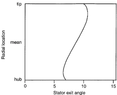
It is characterised by approximately constant angles in the vicinity of the hub and tip and a linear variation between to give a roughly s-shaped distribution. The maximum angle is about 10 degrees near the tip and the minimum is about 7 degrees near the hub which puts the distribution within the ideal range for minimising the diffusion

factors of the second rotor as shown in Figure 4-1. The maximum exit angle of 10

degrees also ensures that the relative tip Mach number of the downstream rotor is not much higher than 1.5. Although this angle distribution was chosen to give the

best aerodynamic results, it is also beneficial from a structural standpoint since the

stator trailing edge is closer to being perpendicular to the wall at the hub and tip

than would be the case for a linear distribution, for example.

The final diffusion factors determnined with the throughilow code were higher than those predicted

tip 0 4u Co, 8 mean CE hub 0 5 10 15

Stator exit angle

Figure 4-2: Stator 1 exit angle distribution

4.1.3

Geometry

Once the flow properties across each blade row were fixed, an estimate of the required area variation was found using a modified form of the corrected mass flow equation also used by Freedman [9],

A2. PtI T 2 MX1 (I + y M2) 2(y-1)(41

- = - -(4.1)

A1 Pt2 Ta Mx2 (1 + 2 IM 12) 2(y-1)

where Mx is the axial Mach number. The use of the total rather than axial Mach

number in the last term is a simple - although not completely accurate - means of

taking into account the effect of swirl. The actual area change that is found by solving differential equations of motion for swirling flow (such as those presented by Anderson,

Heiser and Jackson [2]) is generally smaller than that found with Equation 4.1 so a correction must be applied. This was determined iteratively using the solution from

the throughflow computations, particularly the axial velocity density ratio (Equation

2.16). The value of the axial velocity density ratio should be around one at the hub.

The blade heights were fixed by the compressor throughflow area (neglecting the

tip clearance required for the rotor), but the chord lengths and solidities were among the unconstrained design variables. For all of the blade rows, the hub solidity was set

close to the maximum allowable value to keep the diffusion factors low. Approximately constant chord lengths were used for all blade rows to maximize the solidities away from the hub. The values of the chord lengths were determined from the aspect ratios. These were chosen based on other modern high-speed core compressor designs.

4.2

Flowpath Generation

The large pressure ratios across each stage in this design necessitate area contractions that are much larger than typically seen in axial compressors. This made the flowpath design particularly challenging. Frequently, axial compressors are designed with a constant tip radius which means only the hub is contoured to achieve the required area variation. This minimizes the turning required for a given rate of rotation (because the radii are kept high) and helps keep the losses low. Also, the possibility of the rotor hitting the tip casing during forward-backward vibration is virtually eliminated. However, if the required area contractions are large a constant tip radius leads to a very convoluted profile at the hub. This can adversely affect the flow behavior and increase the structural complexity. Also, there is some benefit to decreasing the tip radius in that it accelerates the flow at the tip and decreases the diffusion factors there. Therefore, for this design a linearly decreasing tip radius was used. The angle of the tip casing relative to the rotational axis is about 3".

Approximate radial coordinates for the hub were determined from the required area (found using Equation 4.1) upstream and downstream of each blade row. Axial coordinates were determined by taking axial projections of the blades and assuming a blade row separation distance of one-quarter of the maximum chord length of the

up-stream blade as suggested by Mattingly [16]. The cubic spline package in MATLAB 2

was used to interpolate between the hub points and generate a smooth flowpath. A major objective in this process was to avoid sharp curves so as to reduce the pos-sibility of flow separation and minimize the pressure gradients caused by streamline curvature. Across the rotors the hub was constrained to be linear to avoid

ical complexity. The linear tip radius decrease lead to a hub ramp angle at the first rotor of about 30'. For the subsequent blade rows, the hub ramp angle decreases approximately linearly.

After the flowpath was initially generated, it was optimised using the results of the throughflow computations (discussed in the next section). This primarily involved further smoothing of the hub profile and small area changes based on the computed axial velocity density ratios. The final flowpath with the axial blade projections is shown in Figure 4-3. 3* STATOR 2 STATOR 1 300 ROTOR 1

Figure 4-3: Flowpath and blades

4.3

Throughflow Analysis

To obtain more accurate estimates for the compressor performance (and improve the design where necessary), the results of the stage design were analysed with a throughflow CFD code. This code was also used to generate the input files for the blade design.

4.3.1

Code Description

The throughflow analysis was performed with MTFLOW, an axisymmetric code de-veloped at MIT by Drela [5]. MTFLOW solves the Euler equations on a streamline grid taking into account the effects of swirl, loss generation, and blockage which are input as spanwise distributions. End wall boundary layers, spanwise mixing, and non-axisymmetric effects are not modelled in the code.

For reference, the 3-D Euler equations in vector form are

80

oP

a

+ + + = pQ (4.2)

where U is the state vector, F, G, and H are the flux vectors in the x, y, and x directions respectively, and

Q

/ \ / Pu pu 2 + P pu~v Puw u(pE +p) / I, p pu pv pw pE I p~v PYLV pv H-pvw v(pE +p) / (4.3)

/

In these vectors, E is the total rotary

0 0

Q2y - 2Qw

Q2z + 2Qv

0

internal energy given by

,1(22 12 E = e+ 1- (U2+ V2 + 2 2) r2 2 2 (4.5) (4.6) \

In MTFLOW, the differential continuity and energy equations (the first and last equa-tions respectively) are not actually solved. Instead a constant mass flow is prescribed along each streamtube to enforce continuity and the total enthaply is prescribed at every point in the flowfield to satisfy the energy equation. These parameters are then used as input to the streamwise momentum equation, which in MTFLOW has the form

dp + pqdq + pVodVo + pd(ZAS) - pd(AW) = 0 . (4.7) With some manipulation, this can be converted to the entropy-convection equation

-pdS + pd(LAS) + pd(AH) = 0 . (4.8)

In MTFLOW either equation can be used, depending on the user's specified prefer-ence.

The geometric inputs required by MTFLOW include the flowpath and axial blade projections. For each blade row, the number of blades and non-dimensionalised wheel speed must also be specified. The blockage, circulation (rv), and adiabatic loss (AS) at each blade row are input as spanwise profiles. The output from MTFLOW includes the positions of streamlines, radial profiles of Mach numbers, flow angles, diffusion factors, and pressure ratios, and actual blade chord lengths (found from the computed flow angles and given axial chord lengths). The pressure contours are also computed. Since some of the quantities computed by MTFLOW are variables that may be inputs to the design process - most importantly in this case the pressure ratios, chord lengths and stator exit flow angles - the results from MTFLOW will not necessarily agree with the initial design intent. The extent to which they do agree is highly dependent on the accuracy of the analysis with which the MTFLOW input values are obtained. Therefore, some iteration is usually required to obtain the desired values.

4.3.2

Results

The pressure contours from the throughflow solution are shown in Figure 4-4. The contours show a high static pressure rise across the second stage as compared to the first stage (due to the higher pressure in the second stage). A region of low static

pressure rise can be seen near the hub of the first stage from rotor mid-chord to stator mid-chord, similar to that seen in Merchant's high-speed aspirated compressor [18]. This is due to the low reaction at the hub. This phenomenon is not seen in the second stage which has less spanwise variation in reaction.

Figure 4-4: Throughflow pressure contours

4.4

Design Summary

The important parameters of the compressor design as determined from the stage analysis and throughflow computations are given in Table 4.1. The overall pressure ratio of the compressor is about 9.2:1 which is short of the initial goal of 10:1, but was the maximum determined to be feasible within the diffusion factor constraints. The pressure ratios and stage loading coefficients for each stage are noticeably higher than those expected for conventional core compressor stages. The reaction for the second stage is also relatively high indicating that the rotor shares a disproportionately high fraction of the loading. The velocity triangles at hub and tip for each blade row are shown in Figure 4-5.

STAGE 1

Rotor Tip Stator Tip

residual swirl

V ' NVb'VN* Va

r

Rotor Hub Stator Hub

residual swirl

NN

STAGE 2

Rotor Tip Stator Tip

%d _or c, Ve

Roor HuNtto u

Figure -5:V

Vd -- - -- - V

- wr

Rotor Hub Stator Hub

/e

Table 4.1: Stage design results

Stage 1 Stage 2

Tip speed 457 m/sec -457 m/sec

Rotor pressure ratio 3.60 2.75

Stage pressure ratio 3.40 2.70

Estimated (average) efficiency 93% 95%

Meanline reaction 0.58 0.72

Flow coefficient 0.58 0.5

Stage loading coefficient 0.70 0.77

Rotor hub solidity 3.5 3.5

Stator hub solidity 3.0 3.0

Inlet corrected mass flow 212 kg/sec -M2

Inlet hub/tip radius ratio 0.5

Outlet hub/tip radius ratio 0.92

Chapter 5

Blade Design

The blade design process involved first designing two-dimensional sections and then stacking the sections radially to produce a three-dimensional blade shape. The blade sections were designed with a turbomachinery cascade code using data extracted from the throughflow solution. This included streamline radii, inlet and outlet flow conditions, chord length, and pitch. In the process of designing the blade sections, an attempt was made to reduce the complexity and difficulty of high-speed aspirated blade design by analysing the relationships between features of previously designed blades.

5.1

Code Description

The blade design code used was MISES, a quasi-three-dimensional turbomachinery cascade solver developed at MIT by Drela et al [7, 25]. In MISES, the flow field is divided into a viscous region, extending from the body surface to a height equal to the displacement thickness of the boundary layer, and an inviscid region outside of this. In the viscous region, the flow is modelled by a two-equation integral boundary layer formulation. In the inviscid region, the flow is governed by the 3-D Euler equa-tions (given in Equaequa-tions 4.2 to 4.5) projected onto an axisymmetric streamsurface of varying radius and thickness. As with MTFLOW, either the standard momentum equation (4.7) or the entropy convection equation (4.8) can be solved depending on

the user's specification. The viscous and inviscid equations are coupled in MISES via the edge velocity and displacement thickness to yield a system of non-linear equations which are solved simultaneously.

In addition to blade analysis, MISES has inverse-design capabilities. Both mixed-inverse and modal-mixed-inverse methods are available, but the former was used in this work. In mixed-inverse design, the desired pressure distribution over a segment of the blade is prescribed by modifying the distribution for a seed geometry. MISES then perturbs the seed geometry at each point to achieve the specified pressure. The camber and thickness of the blade can be preserved during inverse design if desired.

The geometric inputs required for MISES include the blade coordinates and pitch and the radius and thickness of the stream surface on which the blade-to-blade flow is computed. The latter is provided by the throughflow code. The input flow conditions required depend on the boundary conditions imposed and can vary as the calculation proceeds. All of the relevant parameters, including the inlet and outlet Mach numbers, flow angles, and pressures are provided by the throughflow code. For the high-speed blades designed in this work, the boundary conditions generally imposed were the inlet Mach number and pressure, the so-called leading edge Kutta condition (for blades with non-sharp leading edges), the trailing edge Kutta condition and either the inlet flow slope or the exit pressure.

Given the above boundary conditions, the outputs from MISES include cascade exit quantities such as the Mach number, flow angle, and pressure. The viscous and shock losses and the diffusion factor for the blade section are also computed.

In the version of MISES used for this work, the boundary layer formulation in-cludes a suction model. The required inputs to this model are the suction coefficient,

Cm (given by equation 2.25), and the location and length of the suction slot. When

suction is applied it decreases the boundary layer displacement thickness, so it appears as a negative displacement of the streamline at the edge of the viscous layer.

5.2

Design Process

The design process for a blade section is broken up into an inviscid design (represented in MISES by setting the Reynolds number equal to zero) and a viscous design. The steps followed to design the blades in this work are outlined as a flowchart in Figure 5-1.

The process begins with a seed geometry that is generally a previous design that has similar turning (defined as the difference between the exit and inlet flow angles) and inlet Mach number to the present design. A suitable inviscid design is then found by alternately modifying the geometry manually and using the inverse design capabilities of MISES. Often a slightly increased back pressure is imposed during this phase of the design to simulate the effects of viscosity, particularly the deviation of the flow at the blade trailing edge.

For the inviscid design, the geometry modification generally involves choosing the maximum camber to produce the required turning and setting the maximum thickness location based on the shock impingement point. The leading edge radius is chosen according to the inlet Mach number. The stagger angle required to achieve the desired incidence is also found. The choice of these parameters will be discussed in more detail in Section 5.3. The manual geometry modification is performed with XFOIL, an inviscid airfoil design and analysis program developed by Drela [4].

In the inverse design mode, the pressure distribution is modified to match a sub-sonic, transub-sonic, or supersonic template depending on the inlet Mach number. The templates are shown in Figure 5-2 with the important features noted. Inverse design is particularly useful for smoothing the pressure distribution, eliminating pressure spikes at the leading edge where the flow transitions to the pressure and suction sur-faces, and reducing the shock strength by adding precompression. Often the blade shape produced through inverse design has local kinks or bumps. This usually occurs when the pressure distribution is prescribed across a shock. These defects in the blade

surface are smoothed manually using XFOIL.

modification of maximum edge blade smoothing

t

modification of blade shape and trailing edge

modification of maximum camber and thickness, tagger, trailing edge shape

cp

mild pressure gradient

. ... ... . ... _{so nic (M=1)r i (M 1}

No x/c uniform loading

(a) Subsonic

cp smooth deceleration; cp mild precompression

no shock shock

mild pressure gra<

acceleration at

N x/c diverging trailing edge 0 x/c mild pressure gradient

(b) Transonic (c) Supersonic

otherwise can be difficult to detect visually, but will be detrimental to the off-design performance of the blade. The bumps can be located by computing the inviscid pressure distribution over the airfoil using the BLDSET function in MISES. The presence of a bump will result in a local peak in the pressure distribution. An example of a blade with a small bump is shown in Figure 5-3 with the corrected geometry overlayed. The corresponding inviscid pressure distributions are shown in Figure 5-4. The reduction in the pressure spike after the geometry modification can be clearly seen.

3,

Modif ied

Original

0.0 0.0 0.3 0.4 0.5

Figure 5-3: Correction of blade surface bump

RS SINL 0L CM 1.1430 0.2800 -0.0166 -2.0 -1.s CP -1.0 -0.5 0.0 -0.5 1.0

(a) Original blade with bump Figure 5-4: Impact of blade surface

R5

SINL CL CM

1.1430 0.2799 -0.0163

(b) Modified blade with reduced bump bump on inviscid pressure distribution Once an acceptable inviscid design for a blade section is obtained, the viscous solution is computed. The location of the suction slot and the amount of suction are

05 0.2 0.!1 0. 0. 1 _j -2.0 -1.s CP -1.0 -0.5 0.0 0.5 1.01 0. ... - ... ...

chosen so as to prevent the boundary layer from separating. If the boundary layer is found to separate regardless of suction, the inviscid design must be modified. It is generally also necessary to slightly modify the maximum camber and thickness, incidence and trailing edge geometry in the viscous design phase. For supersonic blades, the inviscid solution must usually be re-converged after making geometry modifications and before proceeding with the viscous solution. Although inverse design can be used to modify the viscous design, it is not generally as effective as with the inviscid design, especially for supersonic blades. Inverse design cannot be used (convergence will not be reached) if the boundary layer is separated.

5.3

Blade Features

The main geometric and flow features of a high-speed aspirated compressor blade section are shown in Figure 5-5. Of the geometric variables labelled, only the blade

P2

(a) Geometry parameters (b) Flow parameters

Figure 5-5: Blade section parameters

spacing or pitch, p, inlet and outlet flow angles,

#1

trailing edge geometries, and location and amount of aspiration.

Determining the optimum combination of these parameters to produce the re-quired turning with minimum losses is not a straightforward process and depends heavily on the experience of the designer. As discussed in Section 5.2, the process is generally made easier (and quicker) by beginning with a previously designed blade with similar parameters to those sought. In this work, an attempt was made to reduce the subjectivity of the design process by identifying, and in some cases quantifying, the relationships between various parameters of high-speed aspirated blades. To this end, extensive analysis of the high-speed aspirated blade designs successfully com-pleted by Merchant [18] was performed. These results were used to guide the initial design of some of the blades for the aspirated counter-rotating compressor, however a much larger design space was ultimately explored for the final designs. Therefore, data for these blades was included in the analysis to strengthen the results.

The following sections discuss the issues involved in designing a high-speed aspi-rated blade section with MISES. The focus is on the features that are directly modified in the design process. The relationships presented are useful for obtaining a good ini-tial design for the blade although it is almost inevitable that some modification will be required to obtain the best possible final design. Merchant [18] provides a more detailed discussion of the theory behind the design of each region of the blade.

5.3.1

Incidence

The incidence of the blade is defined as the difference between the inlet flow direction and the projection of the blade camber line at the leading edge

i = 1-Xi (5.1)

The angle of the blade camber line is in turn a function of the camber of the blade and the stagger, , which is the angle of the chordline relative to the axial direction. If the cascade passage is choked and the bow shock is attached to the leading edge of the blade, then the 'unique incidence' condition exists and the inlet flow angle is fixed for a given inlet Mach number, blade thickness, and blade suction surface

angle. As described by Cumpsty [3], the 'unique incidence' inlet flow angle can be found from continuity and the Prandtl-Meyer relation applied along a characteristic

extending from far upstream to the point, e, on the blade where the expansion wave

from the leading edge of the adjacent blade intersects the suction surface,

1 + V (M) = c + v (Me) . (5.2)

To design blades with 'unique incidence' using MISES the cascade exit pressure is constrained and the leading edge geometry and stagger are chosen such that the calculated inlet flow angle matches that provided by the throughflow solution.

For most of the high-speed aspirated blades, the bow shock is actually slightly detached from the leading edge and some spillage of flow between cascade passages is possible. Therefore, the 'unique incidence' flow angle need not be matched exactly (it should be close, however, to keep mass flow capacity and efficiency high). There is also a computational advantage to constraining the inlet flow angle in MISES (to match the throughflow value) rather than the exit pressure and then choosing the leading edge geometry and stagger angle based on other criteria. In particular, it is desirable to minimize spikes in the pressure distribution on the suction and pressure sides of the blade at the leading edge and to reduce the leading edge shock loss (these properties are also affected by the leading edge geometry which will be discussed in Section 5.3.4). It was found in this work that using these criteria gives a blade design for which the 'unique incidence' flow angle matches the angle provided by the throughflow code very closely. This was confirmed by re-computing the flow over a completed blade without the inlet flow angle constrained.

With the leading edge geometry and camber angle fixed by other design consider-ations, the stagger angle is the primary variable used to obtain the correct incidence for the blade. For high-speed aspirated blades, the stagger angle that gives the correct incidence and the turning angle of the blade, (02 - 01), are highly correlated. Figure 5-6 shows the relationship. Once an approximate stagger angle is determined, it must generally be modified slightly throughout the design process as the geometry evolves.