HAL Id: hal-03113862
https://hal.inrae.fr/hal-03113862
Submitted on 18 Jan 2021
HAL is a multi-disciplinary open access
archive for the deposit and dissemination of
sci-entific research documents, whether they are
pub-lished or not. The documents may come from
teaching and research institutions in France or
abroad, or from public or private research centers.
L’archive ouverte pluridisciplinaire HAL, est
destinée au dépôt et à la diffusion de documents
scientifiques de niveau recherche, publiés ou non,
émanant des établissements d’enseignement et de
recherche français ou étrangers, des laboratoires
publics ou privés.
Distributed under a Creative Commons Attribution| 4.0 International License
Rapid measurement of the adult worker population size
in honey bees
Stan Chabert, Fabrice Requier, Joël Chadoeuf, Laurent Guilbaud, Nicolas
Morison, Bernard Vaissière
To cite this version:
Stan Chabert, Fabrice Requier, Joël Chadoeuf, Laurent Guilbaud, Nicolas Morison, et al.. Rapid
measurement of the adult worker population size in honey bees. Ecological Indicators, Elsevier, 2021,
122, pp.107313. �10.1016/j.ecolind.2020.107313�. �hal-03113862�
Ecological Indicators 122 (2021) 107313
1470-160X/© 2020 The Authors. Published by Elsevier Ltd. This is an open access article under the CC BY license (http://creativecommons.org/licenses/by/4.0/).
Rapid measurement of the adult worker population size in honey bees
Stan Chabert
a,b,*, Fabrice Requier
c, Jo¨el Chadoeuf
d, Laurent Guilbaud
a, Nicolas Morison
a,
Bernard E. Vaissi`ere
aaInstitut National de Recherche pour l’Agriculture, l’alimentation et l’Environnement (INRAE), UR406 Abeilles et Environnement, site Agroparc, domaine Saint-Paul, CS 40509 F-84914 Avignon cedex 9, France
bAssociation Nationale des Agriculteurs Multiplicateurs de Semences Ol´eagineuses (ANAMSO), Ferme exp´erimentale, 2485 route des P´ecolets, F-26800 ´Etoile-sur-Rhˆone, France
cUniversit´e Paris-Saclay, CNRS, IRD, UMR ´Evolution, G´enomes, Comportement et ´Ecologie, F-91198 Gif-sur-Yvette, France
dInstitut National de Recherche pour l’Agriculture, l’alimentation et l’Environnement (INRAE), Statistics, UR1052, 67 all´ee des chˆenes, domaine Saint-Maurice, CS 60094, F-84143 Avignon cedex, France
A R T I C L E I N F O Keywords: Apis mellifera Population size Crop pollination Colony collapse Evaluation method Field monitoring A B S T R A C T
Changes in agricultural practices have lead to pollination deficits in entomophilous crops, leading to a growing interest in supplementing farmlands with managed colonies of honey bee, Apis mellifera. However, the metrics of a colony as a pollination unit is controversial due to the wide range of adult population sizes encountered in a colony, especially in relation with the time of year and beekeeping management. Correctly measuring the number of adult honey bees per hive is critical for farmers to adjust the number of colonies they need to meet crop pollination demand. We tested a simple non-invasive method to estimate the adult worker population size of colonies based on common beekeeping handlings. This method consisted in counting the number of inter-frames covered with adult bees (called IFB thereafter) from above the hive body. Based on the monitoring of 181 colonies, we investigated the nature of the relation between IFB and the adult bee population size and its context- dependence to the meterological conditions and hive type. We then evaluated the possible improvement of the method with additional IFB counted in the supers and from below the hive body. Finally, we analysed the robustness of the method by comparing estimates obtained from colonies observed by experimented and naive observers. We revealed a clear-cut logarithmic relation between the IFB and the adult population size, covering the effects of meteorological conditions and hive type. The counting of IFB from above the hive body were particularly sensitive to meteorological conditions, unlike those counted from below the hive body. Moreover, the counting of additional IFB from the supers slightly improved the estimates of adult population size. Inter-estingly, no difference of estimate was detected between experimented and naive observers, suggesting applied simplicity of the method. The IFB counting method thus provides a simple, non-invasive and robust indicator of the adult population size of a managed honey bee colony. The counting of IFB from below the hive body should be recommend due to the sensitivity to meteorological conditions of the counting of IFB from above the hive body. Beyond crop pollination, we also highlighted application perspectives of this method as an indicator of survival probability. This method can therefore be viewed as a standard for routine field monitoring (i) to help farmers to estimate rigorously the number of colonies they need to meet the crop pollination demand and (ii) to help beekeepers assessing the mortality risk of their colonies.
1. Introduction
Over the last century, changes in agricultural landscapes and prac-tices have lead to widespread pollination deficits in pollinator-
dependant crops (Kremen et al., 2002; Garibaldi et al., 2016; Koh
et al., 2016), and to a growing interest in introducing managed
polli-nator species in these crops (Garibaldi et al., 2017). This phenomenon
started at the beginning of the 20th century in USA, where pome fruit
farmers started to rent Apis mellifera colonies from commercial bee-keepers and to introduce them in their orchards as a standard farming
* Corresponding author at: Institut National de Recherche pour l’Agriculture, l’alimentation et l’Environnement (INRAE), UR406 Abeilles et Environnement, site Agroparc, domaine Saint-Paul, CS 40509 F-84914 Avignon cedex 9, France.
E-mail address: stan.chabert@inrae.fr (S. Chabert).
Contents lists available at ScienceDirect
Ecological Indicators
journal homepage: www.elsevier.com/locate/ecolind
https://doi.org/10.1016/j.ecolind.2020.107313
input (Farrar, 1931; Crane, 1999; Kellar, 2018; Ferrier et al., 2018). Since then, farmers have introduced diverse managed insect polli-nator species in entomophilous crops such as bumblebee colonies (Bombus spp.; Hymenoptera: Apidae) and gregarious mason bees (Osmia
spp.; Hymenoptera: Megachilidae) (Garibaldi et al. 2017), but the honey
bee remains the most commonly used species, especially in open fields (Farrar, 1931; Parker et al., 1987; Garibaldi et al., 2009, 2017). The current most common pollinator management practice to reduce polli-nation deficits in crops consists in increasing the stocking rate of honey
bee colonies per unit area of target crop (Rollin and Garibaldi, 2019).
Yet some studies showed that this practice does not necessarily lead to a
reduction in pollination deficit (Degrandi-Hoffman et al., 1987; Viana
et al., 2014; Gaines-Day and Gratton, 2016; Garratt et al., 2018), and it
can even worsen the deficit in some specific cases (Aizen et al., 2014;
Bennett and Isaacs, 2014; S´aez et al., 2014; Grass et al., 2018; Ramos et al., 2018). Delaplane and Mayer (2000) recommended some stocking rates of honey bee colonies per hectare for many entomophilous crops,
based on the mean values recorded in the literature. Yet Farrar (1931)
already questioned a long time ago the relevance of the colony unit when measuring the stocking rate of honey bees, raising “the lack of a uniform standard for measuring colony efficiency”. Indeed, the adult population of honey bee colonies can vary from 10,000 to 65,000 adult
bees (Farrar, 1937). Assessing this adult honey bee population is
therefore a required first step to optimise crop pollination by supplying
the adequate pollinator number (Garibaldi et al., 2020).
To date, three methods have been proposed to estimate the adult worker population size of honey bee colonies. The first consists in weighing the overall adult honey bee population during the night with the counting and weighing of a sample of bees to get their mean indi-vidual weight, the total population being then calculated by a simple extrapolation from this mean individual weight (Farrar, 1937). This method is accurate to estimate the adult population, but it is very time- consuming, it has an unknown impact on the colonies, and it is also challenging to apply routinely in the field due to the night inspections. The second method consists in sequentially removing all the frames
from the hive and weighing the frames with and without bees (Odoux
et al., 2014; Requier et al., 2017), or measuring the frame areas covered
with adult bees, either directly with the human eye (Burgett and
Bur-ikam, 1985; Imdorf et al., 1987; Dainat et al., 2020; Hernandez et al.,
2020), through a grid (Mattila and Seeley, 2007), or through picture
taking and computer-assisted image analysis (Delaplane et al., 2013). In
these latter cases, the adult bee population is calculated by multiplying the frame areas covered with adult bees with the bee density of fully covered frames. This bee density is obtained either by direct bee
weighing (Burgett and Burikam, 1985; Imdorf et al., 1987; Dainat et al.,
2020), or by counting bees in a sampled area (Mattila and Seeley, 2007),
or by measuring the mean surface area of a bee (Hernandez et al., 2020).
These methods are less time-consuming and less restrictive than the first one, but they are also less accurate as the bee density of a fully covered frame can vary substantially (see the different values reported between
Burgett and Burikam, 1985; Mattila and Seeley, 2007; Delaplane et al., 2013; Dainat et al., 2020; Hernandez et al., 2020). Also, it is often used during the course of the day and the adult bee populations assessed can vary with the time of day, the season, and the meteorological conditions. Indeed, the volume of the bee population contained in the colony can be
affected by temperature (Szabo, 1980; Omholt, 1987; Southwick and
Heldmaier, 1987; Sumpter and Broomhead, 2000; Abou-Shaara et al.,
2017), solar radiation (Szabo, 1980; Vicens and Bosch, 2000; Clarke and
Robert, 2018), wind (Pinzauti, 1986; Vicens and Bosch, 2000), and it
varies greatly over the season (Odoux et al., 2014; Requier et al., 2017).
At last, as already stressed by van Dooremalen et al. (2018), this method
is still quite invasive and can impact the colony. For instance, it can disrupt the propolis envelope, which takes part in bee social immunity (Evans and Spivak, 2010), it can cause thermoregulation issues,
espe-cially when ambient temperature is low (Seeley and Visscher, 1985),
and it can lead to a decrease in queen egg-laying or to queen death,
which is especially problematic in autumn or winter while queen
replacement is not possible (van Dooremalen et al. 2018).
The third method, called the “cluster count”, consists in counting, during the day, the number of tops of frames covered with adult honey bees from the top of the hive body (and the number of bottoms of frames from the bottom of the supers when present), without removing the
frames from the hive (Nasr et al., 1990; van Dooremalen et al., 2018).
This method is the simplest and fastest one, and is already commonly used to assess the performance of the colonies introduced for crop
pollination service (McGregor, 1976; Delaplane and Mayer, 2000), and
it has been used recently as a reference for thermographic imaging (Shaw et al., 2011; L´opez-Fern´andez et al., 2018). But no equivalence with the adult bee population size has been provided to date. Overall, to date, no method provides a combination of simple measurement and robust estimate (e.g. including effects of meteorological conditions or hive type) of the adult population of honey bee colonies.
The general objective of our study was to test a simple method, based on the former studies, to enable beekeepers, scientists or any other
observer such as bee brokers (Ferrier et al., 2018) to assess the adult
worker honey bee population size (thereafter called simply bee popu-lation) in a colony and with a particular attention to its practicability for routine use in the field. For this purpose, we adapted the cluster count
method of Nasr et al. (1990) by studying the relation between the
number of inter-frames covered with adult honey bees (IFB) and the bee population, the latter being measured simultaneously using the night
weighing method of Farrar (1937). The only difference between the
cluster count of Nasr et al. (1990) and our IFB count is that the cluster
count consists in counting the number of tops (resp. bottoms) of frames covered with bees from the top (resp. bottom) of the hive body (resp. super), while the IFB count consists in counting the number of spaces
occupied by bees between frames (Fig. 1). Indeed, depending on the
conditions, adult bees may not be distributed over the tops of the frames, but be restricted to the spaces between the frames only. Given that bees are distributed in ellipses in the hive body, with a shift towards the
upper area (Owens, 1971; see also Fig. 8.2 in Seeley, 1985, p. 113), we
first tested the assumption that the IFB increased logarithmically with bee population size. Indeed, the IFB are recorded in one spatial dimen-sion, i.e. on the length of the inter-frames, whereas the bee population grows in two dimensions, on the length and the height of the inter- frames. Secondly, as the bee population does not have the same distri-bution behaviour in inter-frames between the top and the bottom of the
hive (Owens, 1971; Seeley, 1985), we tested the assumption that
recording IFB from below the hive body could lower the estimation error of the bee population compared to that obtained when considering only the IFB counted from above the hive body. We assessed also (i) the reliability of this estimation, and (ii) its robustness against the effects of meteorological conditions, of hive type (Dadant and Langstroth, i.e. two of the most common hive types used worldwide), and of observer experience (experienced versus naive observers). Given that such a simple estimate of the adult population of honey bee colonies can help farmers and beekeepers as an indicator of colony performance for crop
pollination (Geslin et al., 2017; Goodrich and Goodhue, 2020), and of
probability of seasonal and overwintering colony survival (Requier
et al., 2017), we further contextualised the use of this IFB method for crop pollination and honey bee colony losses, as two examples of field- realistic applications.
2. Materials and methods
2.1. Study site, biological model, and hive type
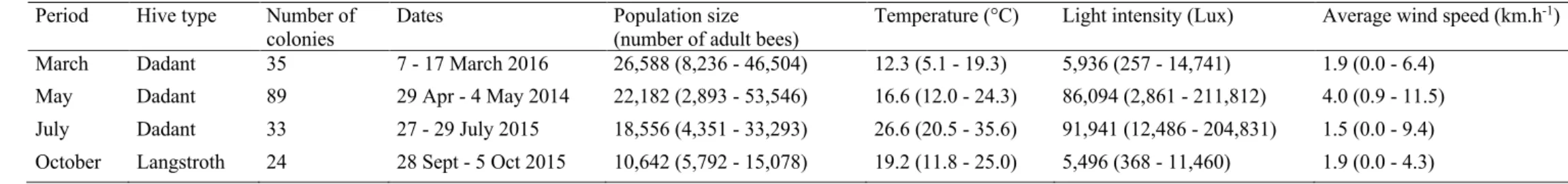
This study was carried out during four periods (i.e. seasons), in May 2014, July 2015, October 2015, and March 2016, on a different apiary in each period, all located close to the INRA centre of Avignon (France). A total of 181 colonies were examined using the same protocol (see below). The number of inspected colonies per apiary is given in
Table A.1.
The hives inspected in March, May and July were of Dadant type, whereas those inspected in October were of Langstroth type. The in-struction given to the beekeepers was to provide us with as many diverse honey bee colonies as possible regarding their bee populations. Both Dadant and Langstroth hives were composed of a 10-frame body, and an 8- or 9-frame super in May and July when the colonies were populous enough, excepted for hives inspected in March and October that never received any super.
2.2. The IFB method – counting the number of inter-frames covered with adult honey bees
The observation of a colony consisted in smoking a little the hive entrance with a bee-smoker, and then lifting the roof and the hive cover with a hive tool ca. one minute afterwards. Then the number of IFB was counted to the nearest half from above the hive body by the observer (Fig. 1a,b). The spaces located at the two external margins of the hive each equated to a half of an inter-frame, so that a maximum number of 10 IFB could be counted overall. The number of IFB could therefore be
equal to 0, 0.5, 1, …, 9, 9.5, or 10, depending on the bee population size. Then the top of the hive body was smoked as necessary and the hive
body was tipped on the side on another hive located nearby (Fig. 1c) or
directly on the floor of the inspected hive. To achieve that, when necessary, the ties binding the bottom board and the hive body were previously removed. In cases where the bottom boards were attached with screws or nails, screws were removed with an electric screwdriver, and nails with a crowbar. The IFB from the bottom of the hive body were
then counted in the same way as from above the hive body (Fig. 1d).
The hive body was then put back in place and re-attached to the bottom board, and the hive closed with its covering and its roof. In the presence of a super, the same kinds of counts were done above and below the super, with a maximum of 9 IFB counted from each side, and the two counts were averaged.
One colony observation took about 3 min per hive without super, and about 5 min per hive with one super, when the bottom boards were attached to the hive bodies with simple ties. When the bottom boards were attached with screws or nails, this time was naturally increased.
Fig. 1. Dadant hive bodies with about 2 (a) and 7 (b) inter-frames covered with adult bees (IFB) counted from above. (c) Dadant hive body tipped on the back side
2.3. Measurement of the bee population
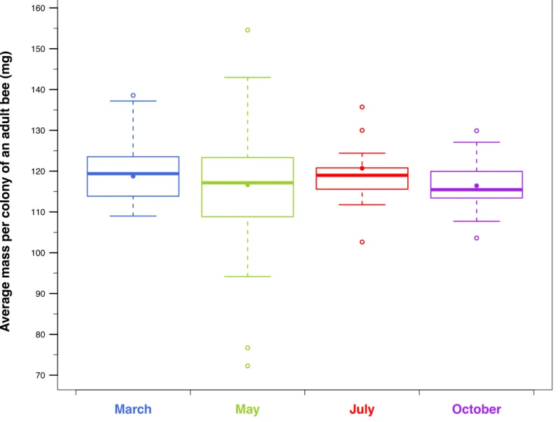
We used Farrar’s method (1937) to measure the adult bee popula-tion. This method required to weigh the total number of adult worker bees contained in the colony. At the end of each of the four periods of colony observations, the frames, super, hive body and bottom board of each hive were shaken and brushed above an empty swarm box at night with the aim to catch all of the adult bees of the colony in the box. This box was then weighed and its empty weight subtracted to get the weight of the bee population. When the bees were returned to their hive, a sample of ca. 100 bees was taken from the population, weighed, and
counted to obtain the mean weight per bee (Fig. A.1). This mean weight
was then used to convert the bee population weight into the number of bees that it contained. Data of bee population weights are summarised by period in Table A.1.
2.4. Relation between IFB and bee population
To establish the relation between the IFB and the bee population size, two situations were analysed separately, (i) hives for which there were no bees in the super, thereafter called ‘without super’, either because the colony was too small, or simply because there was no super, thereby forcing the bees to restrict their distribution to the hive body, and (ii) hives that were equipped with a super, called ‘with super’ (colonies observed during May and July). Colonies insufficiently large for bees to be distributed in a super, but nevertheless equipped with a super, in May and July, were therefore found in both situations. To account for the presence of bees in the super, the average IFB counted from above and below a super was divided by two before being added to the IFB counted in the hive body. We used this figure because the ratio of the area of a Dadant super frame to that of a Dadant hive body frame is 0.55.
Four kinds of piecewise polynomial functions were then made (Bolker, 2008): two functions with two breakpoints for hives ‘without
super’, one breakpoint b1 from which there were enough bees in the bee
population to start to observe IFB, and one breakpoint b2 beyond which
the ten inter-frames of the hive body were saturated with bees, and two
functions with just the first breakpoint b1 for hives ‘with super’. Beyond
the first breakpoint b1, two kinds of relations, linear and logarithmic,
were compared in each situation.
Let y denote the IFB, and let x the bee population. To express y ac-cording to x in hives ‘without super’ with a linear relation:
⎧ ⎪ ⎪ ⎪ ⎨ ⎪ ⎪ ⎪ ⎩ if x < b1,y = 0 if b1<x < b2,y = 10x b2− b1 − 10b1 b2− b1 +ε if x > b2,y = 10 (1) To express y according to x in hives ‘without super’ with a loga-rithmic relation: ⎧ ⎪ ⎪ ⎪ ⎪ ⎪ ⎪ ⎨ ⎪ ⎪ ⎪ ⎪ ⎪ ⎪ ⎩ if x < b1,y = 0 if b1<x < b2,y = 10 ln x ln ( b2/b 1 ) − 10 ln b1 ln ( b2/b 1 ) +ε if x > b2,y = 10 (2)
where b1 is the bee population from which bees start to be visible in
inter-frames, b2 is the bee population beyond which bees saturate the ten
inter-frames of the hive body, and ε is the error parameter.
To express y according to x in hives ‘with super’ with a linear relation:
{
if x < b1, y = 0
if x > b1,y = s(x − b1) +ε (3)
To express y according to x in hives ‘with super’ with a logarithmic relation: ⎧ ⎪ ⎨ ⎪ ⎩ if x < b1,y = 0 if x > b1,y = s ln ( x b1 ) +ε (4)
where b1 is the bee population from which bees start to be visible in
inter-frames, s is the slope of filling inter-frames by bees, and ε is the
error parameter.
The calculations made to obtain Eqs. (1), (2), (3) and (4) are given in
Appendix B.
All the statistics were computed with the software R, version 3.2.0 (R
Core Team, 2015). Asymptotic 95% confidence intervals of parameters of piecewise polynomial functions were estimated with the package
nlstools, version 1.0–2 (Baty et al., 2015).
As simple observations were repeated per colony (see Section 2.6),
the IFB counted during the various observations were averaged per colony. This analysis focused on the data collected by the experienced
observers (see Section 2.8) and on the IFB counted from above the hive
body (+ in the super for hives ‘with super’) in a first analysis, from the bottom (+ in the super for hives ‘with super’) in a second analysis, and on the average of the two (+ in the super for hives ‘with super’) in a third
analysis. Coefficients of determination R2 were calculated for each
relation by the deviance ratio, written as R2D (Nakagawa and Schielzeth,
2013), as well as AIC values (Akaike, 1973; Burnham and Anderson,
2002), to compare linear and logarithmic relations.
2.5. Reliability of estimating the bee population from IFB
To estimate the bee population from the IFB, the converses of the best supported relations previously found (linear or logarithmic) were calculated.
The converses of Eqs. (1) and (3) are of the form:
x =αy + β +ε, withα,β ∈ ℝ andε̃N(0,σ2) (5)
The converses of Eqs. (2) and (4) are of the form:
x = eαy+β+ε, withα,β ∈ ℝ andε̃N(0,σ2)
(Bolker, 2008) which can also be written as:
x =ηeαy+β, withα,β ∈ ℝ andη̃Log − N(0, eσ2)
(6) If the best supported relations previously found were logarithmic, the dependant variable x of the converse relation was transformed in
logarithm to linearise Eq. (6) and enable the estimation of α and β
pa-rameters with a linear model.
Six kinds of explanatory variables y were independently investi-gated: the IFB counted from above the hive body, from the bottom of the hive body, the average of the two, and these three variables with the addition of the mean IFB from the top and the bottom of the super divided by two when a super was present and contained bees. In these last three cases, two converses were estimated: as before, a first one with hives for which there was no bee in the super, called ‘without super’ (see
Section 2.4), and a second one with hives that were equipped with a super, called ‘with super’. As before, there were colonies insufficiently large for bees to be distributed in a super but nevertheless equipped with a super, in May and July, which were therefore in both situations.
To compare the reliability of the six different explanatory variables investigated, some statistics were estimated for each converse relation. As the residual error is constant in the linear Eq. (5) while it depends on the expected value in the exponential Eq. (6), these statistics were estimated differently between the two kinds of relations.
In the case of the relations of type Eq. (5), the three estimated
sta-tistics were: (i) the standard deviation σ of the residual error ε, (ii) the
97.5% quantile of the residual error ε distribution, called Q97.5% and
calculated by the product tγ=97.5%k=n-1 .σ, that express the absolute margin of
and (iii) the minimum number of observations required to estimate the mean bee population of a given apiary with a 95% confidence interval
included in a given margin of error of 10 or 20%, called Nmin-N and
calculated as follows: Nmin− N(x) = ⎛ ⎜ ⎝t k=n− 1 γ=97.5%σ μobsMe 100 ⎞ ⎟ ⎠ 2 (7) where tγk=n-1 is the quantile of γ order of the Student distribution with k
degrees of freedom, µobs is the mean of the bee populations observed, and
Me is the given margin of error in % (here 10 or 20%).
In the case of the relations of type Eq. (6), the four estimated statistics
were: (i) the standard deviation of the residual error η relative to the
expected value, called RSD (x), (ii) the 2.5% and 97.5% quantiles of the residual error η distribution relative to the expected value, called RQ2.5%
and RQ97.5%, that express the asymmetric relative margin of error of
estimating a bee population from IFB with a probability of 95%, and (iii) the minimum number of observations required to estimate the mean bee population of a given apiary with a 95% confidence interval included in
a given margin of error of 10 or 20%, called Nmin-LogN. These four
sta-tistics were calculated as follows:
RSD(x) = 100 ̅̅̅̅̅̅̅̅̅̅̅̅̅̅ eσ2− 1 √ (8) RQ2.5%(x) = 100 et k=n− 1 γ=2.5%σ−σ2 / 2 (9) RQ97.5%(x) = 100 et k=n− 1 γ=97.5%σ−σ2 / 2 (10) Δ(xi) = ( e tk=n− 1 γ=97.5% ̅̅̅̅̅̅̅̅̅̅̅̅̅̅̅̅̅̅σ Nmin− LogN(xi) √ − e tk=n− 1 γ=2.5% ̅̅̅̅̅̅̅̅̅̅̅̅̅̅̅̅̅̅σ Nmin− LogN(xi) √ ) e− σ2 2Nmin− LogN(xi) (11)
where σ2 is the variance of the residual error ε, tγk=n-1 is the quantile of γ
order of the Student distribution with k degrees of freedom. Eq. (11)
does not enable to calculate directly Nmin-LogN according to the margin of
error, but it can be found by testing several values of Nmin-LogN until Δ is
under 10 or 20%. Developments to get Eqs. (8), (9), (10) and (11) are
given in Appendix C.
2.6. Assessment of robustness – effect of meteorological conditions
Robustness describes the ability of an estimator not to be especially
sensitive to small changes in the data or assumptions (Wilcox, 2017; de
Smith, 2018). In other words and in our example, it describes the ability of the IFB to be as reliable to predict the bee population size whatever the changes in the observation conditions.
The ambient temperature was recorded every 5 min throughout the overall duration of observations by a sensor HOBO® Pro v2 (Onset® Computer Corporation, USA) placed under shelter near the apiaries. The light intensity was recorded every minute in lux during the same period and at the same place by a sensor HOBO® Pendant (Onset® Computer Corporation, USA) placed horizontally in broad daylight. The light in-tensity was then converted to relative light inin-tensity, that is by dividing the instant light intensity by the maximum instant light intensity recorded during one period. This helped to overcome strong differences in light intensity between periods. The average wind speed was recorded from the beginning to the end of colony observations and for each half- day, by an anemometer SKYWATCH® Eole (JDC Electronic SA, Switzerland) placed two meters high at the end of a telescopic tripod
near the apiaries. These data are summarised by period in Table A.1.
Simple colony observations were repeated between four and seven times
per colony, each time on a different but consecutive day (see Table A.1
for dates), to enable to test the effect of meteorological conditions on IFB on a given colony. Repeated colony observations alternated between morning and afternoon in a given period.
To test if the meteorological conditions impacted the IFB, the IFB counted from above and from below the hive body were modelled by a generalized linear mixed model (GLMM) approach using a binomial distribution. The fixed explanatory variables were, in order, the bee population in interaction with the period to test if the filling rate of inter- frames by bees changed according to the period or to the hive type (the ratio of the area of a Langstroth frame to that of a Dadant one is 0.79),
the ambient temperature (in ◦C), the relative light intensity (averaged
over the 60 min preceding the observation, in %), the average wind
speed over the half-day of observation (in km.h−1), the temporal shift
between observation and bee population weighing (in days) in inter-action with the period to take into account the potential evolution of the bee population during this time, and so the period. As colony observa-tions were repeated by colony, the colony number was set as a random explanatory variable. Four GLMMs were generated to test the impact of meteorological conditions on the IFB counted from above and from below the hive body by both experienced and naive observers. GLMMs
were generated with package lme4, version 1.1-14 (Bates et al., 2015b).
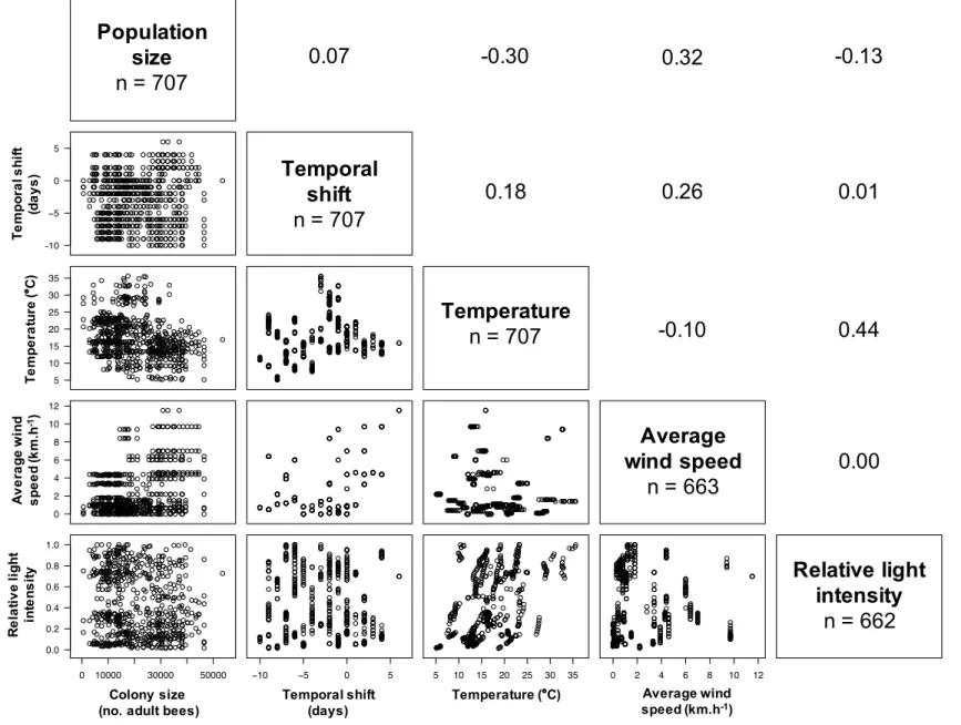
To check for collinearity between fixed explanatory quantitative variables, two variables were incorporated together in GLMMs only if
absolute value of correlation coefficient was less than 0.7 (Dormann
et al., 2013). Fig. A.2 displaying correlation coefficients values was
generated with package Rarity, version 1.3–6 (Leroy, 2016). To
stan-dardize effect sizes, fixed explanatory variables were centered and
standardized (Schielzeth, 2010).
As the null hypothesis significance testing approach is discussed (e.g.
Stephens et al., 2007; Stanton-Geddes et al., 2014; McShane et al.,
2019), we set the p value threshold to 0.001 in order to be more
con-servative (Johnson, 2013). Effect size and 95% confidence intervals
were also reported (Nakagawa and Cuthill, 2007). 95% confidence
in-tervals were estimated with the Wald method (Bates et al., 2015a).
Marginal R2 values were also calculated, written as R2GLMM(m) (
Naka-gawa and Schielzeth, 2013).
2.7. Assessment of robustness – effect of hive type
To test whether the hive type affected the filling rate of inter-frames by bees in relation with the bee population size and therefore the rela-tion between IFB and bee popularela-tion, the colony observarela-tions and the weighing of the bee population were made on two hive types, Dadant (N
=157) and Langstroth (N = 24). We could not sample more Langstroth
hives, as it was not the hive type mainly used by the beekeepers who provided us with the colonies. Dadant and Langstroth frames have different areas that can affect the filling rate: the ratio of the area of a Langstroth frame to that of a Dadant one is 0.79, so a Langstroth frame should fill up in bees 1/0.79 = 1.3 times faster with the same bee population than a Dadant frame. To compare the filling of inter-frames by bees regarding the bee population between the Dadant and Lang-stroth hives, the relation between the IFB and the bee population found for the Langstroth type was divided by the one found for the Dadant type on the range of bee populations sampled in common for both types (see
Table A.1). The Dadant hive was investigated during March, May and July, while the Langstroth hive was investigated in October. The period of October was therefore mixed up with the hive type.
2.8. Assessment of robustness – experienced versus naive observers
To test if the estimation of a bee population from the IFB was objective and if the robustness regarding the variations of the meteo-rological conditions was an objective pattern, the colony observations were performed each time by two kinds of observers: those who had already experience in beekeeping or had already applied the IFB method, which we called experienced observers, and naive ones, new to both situations. Both types of observers counted independently. The
statistics presented in Section 2.5 were compared between the two kinds
was similar or not to that of the experienced observers.
2.9. Application for ecological issues of colony loss and crop pollination
We used the BEEHAVE model (Becher et al., 2014) to illustrate the
interest of recording the IFB as an ecological indicator of colony survival and crop pollination performance. A total of 200 simulations of colony dynamics were computed during a complete year, with a Dadant hive type and ad libitum addition of supers. We first calibrated the model with
Becher et al.’s (2014) initial colony settings, i.e. European conditions of climate and landscape composition, associated with a random parame-terisation of the initial population for model stochasticity. To do so, we randomly attributed an initial adult population ranging from 9,000 to
13,000 bees on January 1st. In order to consider beekeeping
manage-ment conditions, we also enabled the ad-hoc options such as the Varroa
destructor mites treatment and the honey harvests.
Then, we ran the simulations in two lots, the healthy colonies (n = 100 simulations) and the disturbed colonies (n = 100 simulations), by a change in demographic and health parameters on the first day of simulation (and then applied them during the complete run). Healthy colonies consisted in simulations with random-boost of colony de-mographic rate and individual survivorship, and the absence of Varroa
destructor infestation. The boost of the colony demographic rate was
computed with an increase of the maximum egg-laying capacity of the queen between 1,600 and 1,800 eggs per day (default value of 1,600 eggs per day). The boost of the survivorship of bees was computed with a
decrease of the probability of worker larvae mortality between 3/103
and 1/102 per day of larvae development (default value of 1/102 per day
of larvae development), and with a decrease of the probability of forager
mortality between 7/106 and 1/105 per second of flight (default value of
1/105 per second of flight). The disturbed colonies consisted in
simu-lations with random-weakening of colony demographic rate (between 1,400 and 1,600 eggs per day) and individual survivorship (between 1/
102 and 3/102 per day of larvae development and between 1/105 and 3/
105 per second of flight), and an infestation with 2 to 10 Varroa
destructor mites/100 bees from which the prevalence of virus-infected
mites ranged from 30% to 50%.
The colony dynamics of the total number of bees was then converted
into a number of IFB inferred with Eq. (4), since the simulations included
supers and the below view turned out to be more robust (see results). The BEEHAVE model estimated the number of forager bees (an indicator of crop pollination performance) that was also converted into IFB. Simulation endpoints that were deemed insufficient for colony survival, i.e. the risk of colony collapse, were estimated through two following
thresholds according to Becher et al. (2014): (i) simulations that reach
population size smaller than 4,000 adult bees during the winter, and (ii) simulations that reach a null amount of honey stock during the winter season.
3. Results
A total of 181 colonies were observed during the four periods, with bee populations ranging from 2,893 to 53,546 adult bees, and a smaller
variability in October (Table A.1). As colonies had time to grow during
the temporal shift between the first colony observations and the bee population weighing in March, the observations made with a temporal shift strictly greater than four days were removed in the analyses of the
Sections 3.1 and 3.2 (see Section 3.3).
3.1. Relation between IFB and bee population size
The logarithmic relations between IFB and bee population were
systematically better supported than the linear ones by R2
D and AIC
values (all ΔAIC values > 9) in the Dadant hives observed by the experienced observers. This was true regardless of the observation considered, that is the IFB counted from above the hive body, from
below, the average of the two, or when also considering the bees con-tained in the super (Table A.2; Fig. 2).
Conversely, the linear relations were better supported, but with much less support (all ΔAIC values < 2), than the logarithmic ones in the Langstroth hives (Table A.2).
Bees started to be visible with a smaller bee population by observing the Dadant hive body from above than by observing it from below, ac-cording to the logarithmic relations in hives with or without super (Table A.2). However, the ten inter-frames were saturated with the same bee population on the top or the bottom of the hive body in Dadant hives without super. The filling rate of inter-frames by bees with the increase of the bee population was also higher when counting the IFB from below the hive body (plus in the super) than counting from above (plus in the super) in Dadant hives with a super.
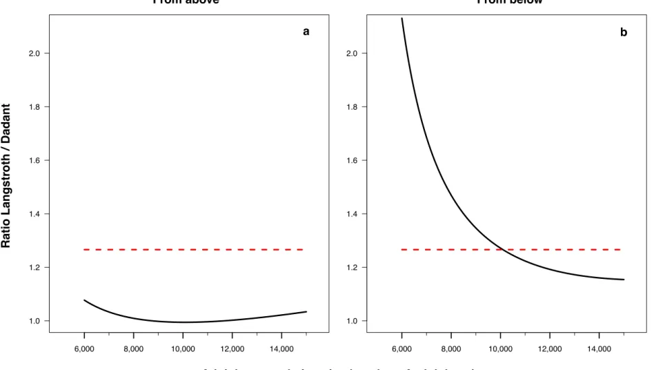
The filling rate of inter-frames by bees regarding the bee population size was nearly the same in Langstroth and Dadant hives when counting the IFB from above the hive body on the range of bee population sizes
included between 6,000 and 15,000 bees (Fig. 2a and A.3a). This rate
was, however, between 1.1 and 2.1 times higher in Langstroth hives compared to Dadant hives when counting the IFB from below the hive body, with a ratio approaching 1.3 between bee populations of 8,000 and 12,000 bees (Fig. 2b and A.3b).
In Dadant hives with or without super, the models with the best R2D
values were those where the IFB considered were those counted only
from below the hive body (Table A.2). In Langstroth hives, the models
with the best R2D values were, however, those where the IFB counted
from above and below the hive body were averaged.
3.2. Reliability of estimating the bee population from the IFB
Only the converses of the best supported types of relations found in
Section 3.1 were investigated in the following analyses, i.e. the expo-nential relation for Dadant hives, and the linear relation for Langstroth hives.
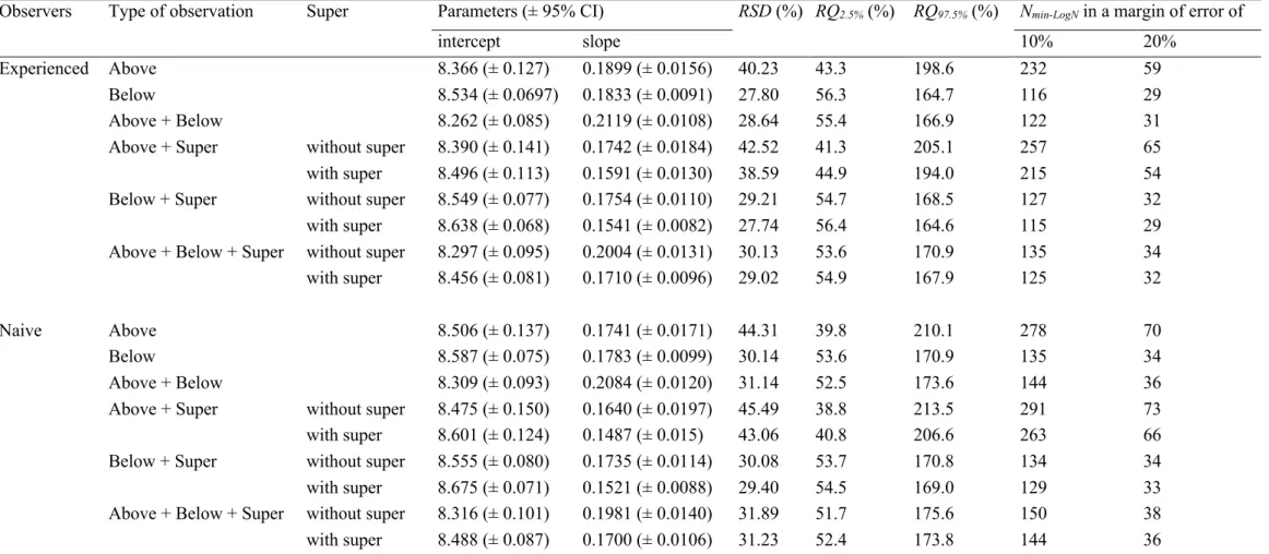
When disregarding the bees contained in the super, the kind of
observation with the smallest RSD, RQs or Nmin-LogN values in Dadant
hives observed by the experienced observers was the one with the IFB
considered from below only (Table A.3). Considering the averaged IFB
counted from above and below increased the estimation error. And considering only the IFB counted from above only increased even more this error. When including bees contained in the super, still in Dadant hives observed by the experienced observers, we observed the same pattern. There was in that case a little reduction of the error of estima-tion compared to when the bees contained in the super were not taken into account, considering the IFB counted from above only or from
below only (Table A.3). The RSD was 27.7% in this latter case, with an
error that varied between − 56% and +165% in 95% of the cases at the colony level. But this error gap can be reduced to 10 or 20% to estimate the mean bee population of colonies in an apiary, by sampling 115 or 29 colonies in this apiary (Table A.3).
The same pattern was observed again for Dadant hives inspected by
the naive observers, with higher RSD, RQs or Nmin-LogN values compared
to when colonies were observed by the experienced observers (Table A.3).
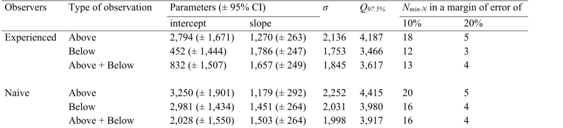
As for Dadant hives, the type of observation with the smallest σ,
Q97.5% or Nmin-N values in Langstroth hives observed by the experienced
observers was the one with the IFB recorded from below only (Table A.4). And still, as for Dadant hives, considering the averaged IFB counted from above and below increased the estimation error, and considering only the IFB counted from above increased even more this error. On the other hand, in Langstroth hives observed by the naive
observers, σ, Q97.5% or Nmin-N values were the smallest when the IFB
counted from above and below were considered both and averaged. The estimation error was slightly increased when the IFB was considered only from below, and it was even more when the IFB was considered only from above (Table A.4). Finally, σ, Q97.5% or Nmin-N values were
higher for the Langstroth hives observed by the naive observers than for
those observed by the experienced observers (Table A.4).
3.3. Assessment of robustness
We were able to cover a relatively large array of meteorological
conditions, from 5.1 to 35.6 ◦C for temperature, 257 to 211,812 Lux for
light intensity, and 0 to 11.5 km.h−1 for wind speed.
All the fixed explanatory quantitative variables investigated could be integrated together in models because of values of correlation
co-efficients among them less than 0.7 (Fig. A.2). The IFB counted from
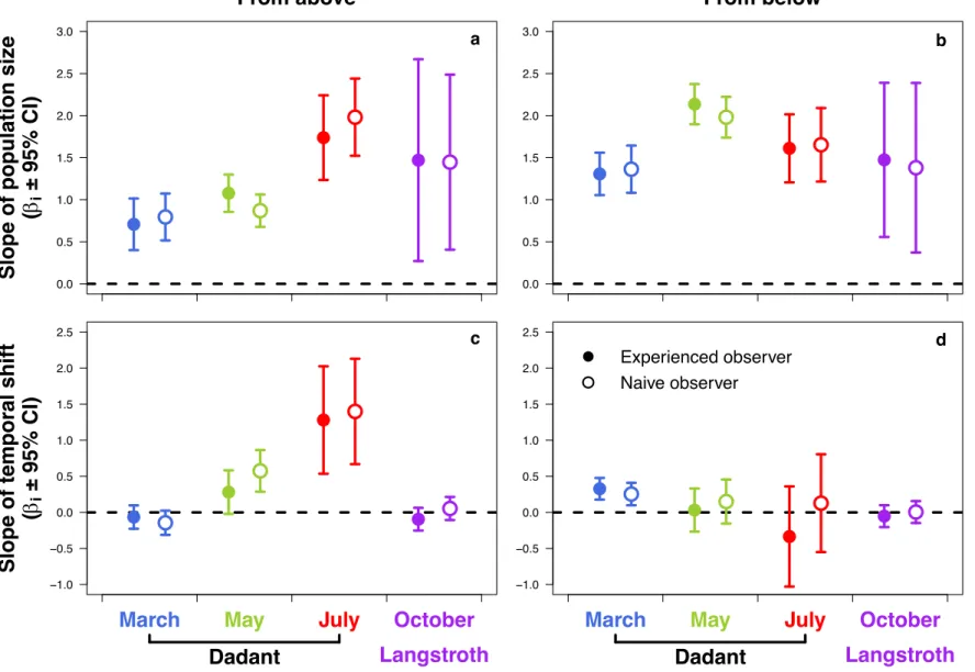
above and below the hive body was dependant first on the bee popu-lation, during the four periods and for the two kinds of observers (Table 1 and Fig. A.4). Colony observations from below were, however, more robust to meteorological conditions than from above. The IFB counted from above increased with the temperature, and decreased with the relative light intensity for both experienced and naive observers, with a more markedly slope for temperature, while the IFB counted from
below did not (Table 1). The IFB counted from above increased
more-over with the temporal shift between observation and bee population weighing during the period of July in the two types of observers, as well
as the IFB counted from below during the period of March (Fig. A.4). The
marginal R2
GLMM(m) values were higher in models with the IFB counted
from below than from above, for the two types of observers (Table 1).
According to these results, the observations made with a temporal shift between observation and bee population weighing greater than
four days during the period of March were removed from the analyses of
the previous Sections 3.1 and 3.2, to avoid an unwanted effect observed
on the IFB counted from below. No observations were removed for the period of July, despite a similar effect on the IFB counted from above, because the temporal shifts between observation and bee population weighing were all less than four days.
3.4. Application for ecological issues of colony losses and crop pollination
Our simulations showed the ability of the IFB to discriminate the
population dynamics of healthy vs. disturbed colonies (Fig. 3a). While
healthy and disturbed colonies started the simulations with the same bee population of 4.90 ± 0.52 (µ ± sd) IFB from below the body of a Dadant hive (i.e. 10,920 ± 1,058 adult bees), these two batches of simulations (n = 100 for each) fitted different temporal patterns. The healthy col-onies increased their population during the year, reaching a total of 10.44 ± 0.79 IFB (i.e. 31,294 ± 4,611 adult bees) at the peak of colony
growth (from July 15th to September 15th), and finished the year with an
annual increase of 0.47 ± 1.26 IFB (i.e. 1,235 ± 2,811 adult bees). On the other hand, the disturbed colonies showed a weakened temporal pattern with 3.18 ± 2.74 IFB (i.e. 9,138 ± 5,183 adult bees) at the peak of colony growth, and an annual decrease of 4.62 ± 0.87 IFB (i.e. 16,834
±6,971 adult bees). Interestingly, the BEEHAVE model allows to
esti-mate the forager strength of the honey bee colony at a given date. Beside the estimation of the bee population, the IFB could inform on the forager strength of the honey bee colonies, this later varying between healthy
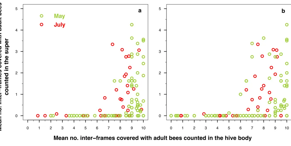
Fig. 2. Relations between the mean number of inter-frames covered with adult bees (IFB) counted by the experienced observers and the bee population, given for
colonies without super or without adult bees contained in the super when present (a, b), and for colonies equipped with a super (c, d). The IFB were counted from above (a, c) or from below the hive body (b, d). Solid lines represent the mean predictions of piecewise polynomial functions (Table A.2; see Eqs. (2) and (4) for black lines, and Eq. (1) for purple lines). Dadant and Langstroth are the two hive types tested.
colonies (10,878 ± 2,650 forager bees) and disturbed colonies (2,163 ±
1,381 forager bees) at the peak of colony growth (Fig. 3b). The
simu-lated healthy colonies showed 100% survival over the year instead of
27% for the disturbed colonies (Fig. 3c), and the estimated IFB at the
peak of colony growth was positively correlated with the colony survival (GLM with a binomial error distribution; n = 200, z = 3.364, p = 0.00073). Thus, the measure of the IFB at a given date can be viewed as an indicator of colony survival.
4. Discussion
We found a logarithmic relation between the IFB and the adult population size of a colony, regardless of the presence or not of a super. This result is consistent with our assumption that the more the colony and its bee population grow, the more the bees cover the entire surface of the frames they fill, and the less they fill new inter-frames. However, the best supported relation in Langstroth hives was the linear one, but with little evidence compared to the logarithmic relation. This most probably comes from the fact that the colonies inspected to test this hive type had a quite low size variation range (ranging from 6,000 to 15,000 bees only), as they were inspected in October, a period during which colonies have a quite low size.
The estimates of adult population of honey bee colonies, derived from the IFB method, are consistent with previous data. The inspected colonies were of very different sizes during March, May and July, ranging from nearly 3,000 adult bees for the smallest one, to nearly 53,500 bees for the largest one. These values are consistent with the
extrema described in the Schmickl and Crailsheim’s (2007) model of
honey bee population dynamics, that were of about 5,500 and 50,000 bees. They are nearly consistent too with the extreme values reported in
Farrar’s (1937) study, that were of about 10,000 and 65,000 bees. The
proposed method allows to count some IFB in 10-frame Dadant hive body from nearly 1,500 bees contained in the colony when counting from above, and from nearly 4,000 bees when counting from below. This
is in agreement with Owens (1971) who found that bees distributed
themselves in the hive with a shift towards the upper area using the measure of isothermal curves.
The filling of inter-frames by bees in relation with the bee population seemed nearly the same in the Langstroth and the Dadant hives when counting the IFB from above the hive body on the range of bee pop-ulations encountered in the Langstroth hives, while it was more variable when counting the IFB from below the hive body, between 1.1 and 2.1 times higher in the Langstroth hives compared to the Dadant ones. This ratio seemed to approach the 1.3 value between bee populations of 8,000 and 12,000 bees, corresponding to the ratio of the area between a the Dadant frame and a Langstroth one. The study should be neverthe-less extended beyond the range of populations encountered in the Langstroth hives to be able to generalise these ratio.
Also, the filling of inter-frames by bees was robust to the meteoro-logical conditions on the bottom of the hive body, whereas it largely depended on the temperature and light intensity on the top, regardless of the experience of the observers. Indeed, the higher the temperature was, the more the bees dispersed themselves in the inter-frames on the top of the hive body. This is in agreement with the dispersion of the bee
population when the temperature rises above 15◦–18 ◦C (Seeley, 1985;
Southwick and Heldmaier, 1987; Sumpter and Broomhead, 2000). The effect of the decreasing in bees contained in the nest by the increase of
the honey bee foraging activity with temperature (Szabo, 1980; Corbet
et al., 1993; review in Abou-Shaara et al., 2017; Nielsen et al., 2017) is therefore negligible compared to the effect of the dispersion of the bee population. To a lesser extent, the higher the relative light intensity was, the fewer the bees observed in the inter-frames on the top of the hive
Table 1
Statistics of the GLMMs computed to test the effect of the meteorological conditions on the number of inter-frames covered with adult bees (IFB) counted from above and below the hive body by the two kinds of observers.
Type of observation Predictor Modality Experienced observers Naive observers
Estimated parameter (±95% CI) z p Estimated parameter (±95% CI) z p
From above Intercept March 2.266 (±0.322) 13.80 <0.001 2.277 (±0.290) 15.50 <0.001
Population size 0.708 (±0.307) 4.52 <0.001 0.795 (±0.281) 5.59 <0.001
Temperature 0.547 (±0.134) 8.00 <0.001 0.535 (±0.136) 7.74 <0.001
Relative light intensity − 0.213 (±0.077) − 5.41 <0.001 −0.204 (±0.076) −5.27 <0.001 Average wind speed − 0.041 (±0.083) − 0.96 0.335 −0.078 (±0.081) −1.89 0.0588
Temporal shift − 0.065 (±0.162) − 0.79 0.432 −0.144 (±0.168) −1.69 0.0919
Period May − 1.021 (±0.522) − 3.83 <0.001 −1.457 (±0.470) −6.08 <0.001 July − 2.255 (±0.675) − 6.55 <0.001 −2.503 (±0.628) −7.79 <0.001 October − 0.577 (±1.223) − 0.93 0.355 −0.483 (±1.050) −0.89 0.372 Population size × Period May 0.369 (±0.377) 1.92 0.0555 0.076 (±0.340) 0.44 0.660
July 1.033 (±0.590) 3.43 <0.001 1.188 (±0.510) 4.34 <0.001
October 0.759 (±1.238) 1.20 0.230 0.645 (±1.087) 1.17 0.241
Temporal shift × Period May 0.346 (±0.379) 1.79 0.0733 0.719 (±0.369) 3.81 <0.001 July 1.346 (±0.783) 3.37 <0.001 1.550 (±0.767) 3.94 <0.001 October − 0.029 (±0.214) − 0.27 0.789 0.198 (±0.220) 1.76 0.0781
R2
GLMM(m) =0.250 R2GLMM(m) =0.260
From below Intercept March 1.599 (±0.252) 12.45 <0.001 1.702 (±0.276) 12.19 <0.001
Population size 1.307 (±0.252) 10.17 <0.001 1.363 (±0.284) 9.51 <0.001
Temperature 0.114 (±0.128) 1.74 0.0821 0.105 (±0.131) 1.57 0.117
Relative light intensity − 0.057 (±0.074) − 1.50 0.134 −0.077 (±0.074) −2.03 0.0421
Average wind speed 0.069 (±0.080) 1.68 0.0928 0.088 (±0.081) 2.12 0.0342
Temporal shift 0.327 (±0.150) 4.27 <0.001 0.254 (±0.155) 3.21 0.00134
Period May − 0.470 (±0.473) − 1.95 0.0513 −0.703 (±0.489) −2.82 0.00476
July − 0.236 (±0.597) − 0.78 0.439 −0.906 (±0.595) −2.98 0.00289 October 0.049 (±0.943) 0.10 0.918 −0.286 (±1.018) −0.55 0.583 Population size × Period May 0.829 (±0.344) 4.72 <0.001 0.618 (±0.373) 3.29 0.00101
July 0.303 (±0.476) 1.25 0.212 0.289 (±0.495) 1.09 0.274
October 0.166 (±0.950) 0.34 0.731 0.004 (±1.060) 0.01 0.993
Temporal shift × Period May − 0.296 (±0.365) − 1.59 0.112 −0.104 (±0.374) −0.54 0.587 July − 0.674 (±0.733) − 1.80 0.0715 −0.130 (±0.715) −0.35 0.723 October − 0.380 (±0.201) − 3.71 <0.001 −0.250 (±0.204) −2.40 0.0166
R2
GLMM(m) =0.449 R2GLMM(m) =0.448 All of the quantitative explanatory variables were centered and standardized. R2
body. This is in agreement with the increase of the honey bee foraging
activity when solar radiation rises above 300 W.m−2 (Vicens and Bosch,
2000; Clarke and Robert, 2018). Although the foraging activity of honey
bees decreases sharply beyond 10 km.h−1 of wind speed (Pinzauti, 1986;
Vicens and Bosch, 2000), the wind speeds measured during our obser-vations were relatively small, this not permitting to conclude to a wind speed effect on the IFB counted from above or below the hive body.
Interestingly, the assessment of the robustness of the method showed that using a view from below the hive body improved the estimate of the bee population from the IFB, in comparison to using an above view, or using the average of above and below views. Considering the IFB in the super when present enabled to improve a little more this estimation. The most relevant and effective method consisted therefore in choosing, either to count, ideally, the IFB from the single bottom of the hive body when it is possible and by adding the IFB in the super when present, or to count the IFB from the single top of the hive body when counting from the bottom is too challenging (e.g. when the floor is attached to the hive body with screws or nails), with adding also the IFB in the super when present. The estimation error is quite high at the colony level, but it can be reduced at an apiary level by sampling several colonies, to assess with
a better reliability the mean bee population of the apiary.
This estimation was quite objective, as the estimation error was similar between experimented and naive observers. The estimation error was nevertheless slightly lower for the experienced observers than for the naive ones. The study should be continued for the Langstroth hive type and extended beyond the range of populations encountered. Furthermore, as the naive observers recorded a little more variable IFB than the experienced observers, it is recommended for naive observers to practice the method on a few colonies before using it routinely.
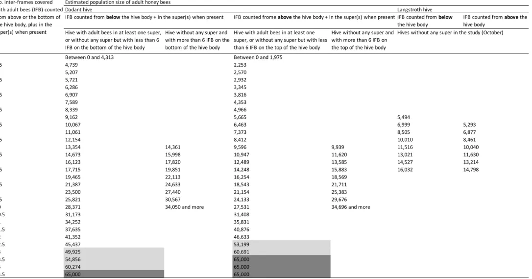
The reliability estimates in Langstroth hive type gave the same re-sults, with the slight difference that the estimation was better when averaging the IFB counted from above and below the hive body for the observations of the naive observers. But the estimation errors between the IFB counted from above and below averaged and the IFB counted from below only were quite similar. This therefore does not really call into question the previous conclusions. However, a conversion is necessary to cross estimate the bee population from the counting of the IFB on Dadant and Langstroth hive types. As bees filled super when present only when they filled at least six inter-frames on the top or the bottom of the hive body (Fig. A.5), the physical coercion (i.e. the spatial
Fig. 3. Integrating the number of inter-
frames covered with adult bees (IFB) in estimates of honey bee colony survival and crop pollination. (a) The simulated yearly population dynamics of healthy and disturbed honey bee colonies expressed as IFB inferred from below the hive body (Eq. (4)) and a Dadant hive type. Thick lines show the average value of the simulations (n = 100 healthy col-onies and n = 100 disturbed colcol-onies) at day d with shaded areas indicating the 95% confidence intervals. (b) The IFB indicate the total number of adult bees and the foraging strength of the colony (i. e. the number of forager bees). We show the averaged value per colony at the peak of colony growth (from July 15th until
September 15th). (c) The IFB at the peak
of colony growth increase survival of simulated bee colonies (GLM with Bino-mial error distribution: p < 0.001). The line represents the model fit while the shaded area show the 95% confidence interval.
limit) of the hive body of limited volume should apply on the relation between the IFB and the bee population only beyond six inter-frames filled on the top or the bottom of the hive body. This is therefore only from this threshold of IFB that the relation between the IFB and the bee population should be different between hives with and without supers. This is the reason why the conversion between the IFB and the bee
population in hives without super is given only from six IFB (Table A.5).
Below this threshold, one can refer to the conversion given for hives equipped with a super. It is also worth to note that the estimated bee population given for hives containing more than 13 IFB counted from below the hive body, or 12.5 from above, were approximate, as the relation is exponential, and as a colony of more than 45,000 bees is quite
exceptional (Table A.5). The maximum estimated bee population
pro-posed is 65,000 bees, as it is the maximum observed by Farrar (1937).
This method may help to better manage crop pollination service by introducing the appropriate amount of adult honey bees in a given crop area to minimise pollination deficits, in addition to the wild pollinators already present in the environment of the target crop, as recommended
in the Integrated Crop Pollination concept (Isaacs et al., 2017). Indeed,
Geslin et al. (2017) showed that honey bee colonies with a higher IFB counted from above the hive body increased apple flower-visitation rates by honey bees, and subsequent fruit set, seed set, fruit sugar
con-tent and farmers’ profits. And Goodrich and Goodhue (2020)
high-lighted that nearly 100% of almond growers in California request honey bee colonies with a minimum population level in their pollination contracts. This would lead to redefine the currently used unit of managed honey bee colonies introduced per unit area of target crop to reach a stocking rate aiming at the direct number of adult honey bees required per unit area. This would enable beekeepers to manage their beekeeping operations better, for instance by introducing more small colonies to make them grow during the crop flowering.
As a perspective, it would be relevant to investigate the foraging population of a honey bee colony in relation to its size. Indeed, the adult population includes various bee castes that provide different work tasks from in-nest work (e.g. nest cleaning, brood rearing) to external tasks such as the flight learning, patrol flights, and foraging flights that are probably the best indicator of colony performance from a crop pollina-tion standpoint. By using bee colony simulators, such as the BEEHAVE
model (Becher et al., 2014), it is now possible to predict the number of
forager bees in the adult population of honey bees, and therefore to go further in the estimate of colony performance for pollination service. Moreover, combining the IFB method with such simulations provides a tool for beekeepers to anticipate and mitigate the colony mortality, a
current issue worldwide (Potts et al., 2010; Goulson et al., 2015). It is
well-established that the adult population of honey bee colonies is a good indicator of the health status of a colony, and also can be used as an early-warning signal of the probability of seasonal and overwintering
colony mortality (Requier et al., 2017; D¨oke et al., 2019). Thus, the IFB
counting method provides a simple and robust indicator of the adult population of a managed honey bee colony with perspectives of field- realistic applications in the current context of crop pollination deficit and honey bee colony losses. With the recent application of
thermo-graphic imaging to the assessment of honey bee population (Shaw et al.,
2011; L´opez-Fern´andez et al., 2018), it can also enables one to convert a radiation level of a colony into a number of honey bees.
5. Conclusion
Counting the IFB constitutes a simple, fast, non-invasive and quite robust method to assess routinely the adult population size of a honey bee colony in the field, for any kind of observer such as beekeepers, scientists or bee brokers. This method can be viewed as a standard for routine field monitoring in the current context of crop pollination def-icits and honey bee colony losses, as two examples of field-realistic ap-plications. It is recommended to favour the IFB counted from below the hive body, whenever possible, against the counts made from above, and
to add the IFB counted in the super when it is present. It is also rec-ommended for naive observers to practice the method on a few colonies before using it routinely, in order to reduce the estimation error. The number of managed adult honey bees introduced per unit area of target crop for pollination service should therefore be used as a more relevant variable than the mere stocking rate of honey bee colonies. This unit will enable to better coincide the overall supply of insect pollinators, including managed and wild insect pollinators, with the pollination re-quirements of a given target entomophilous crop.
Author contributions
B.E.V., S.C., and F.R. conceived the idea and designed the method-ology, S.C., L.G., and B.E.V. collected the data, N.M. provided assistance for temperature and light intensity recordings, S.C. and J.C. analysed the data, F.R. performed the simulations, S.C., F.R., and B.E.V. wrote the manuscript. All authors gave final approval for publication.
Funding
This work was supported by the European Agricultural Guarantee Fund (EAGF) as part of the French National Apiculture Programme [FranceAgriMer convention number 14-05 R], and by the Association Nationale de la Recherche et de la Technologie (ANRT) as part of the Conventions Industrielles de Formation par la REcherche (CIFRE) doctoral grants [convention number 2014/0070], allocated here to S.C. by the Association Nationale des Agriculteurs Multiplicateurs de Semences Ol´egineuses (ANAMSO) through the specific interprofessional actions with the Groupement National Interprofessionnel des Semences et plants (GNIS) and the Union Française des Semenciers (UFS). The funders had no role in study design, data collection and analysis, deci-sion to publish, or preparation of the manuscript.
Declaration of Competing Interest
The authors declare that they have no known competing financial interests or personal relationships that could have appeared to influence the work reported in this paper.
Acknowledgements
We thank all the beekeepers for providing us with the colonies to carry out this study or preliminary works, Simon Bellot, Raymond Ber-nadet, Philippe Dauzet, Cyril Folton, Alexandre Gorit, Eric Lelong, Sonia Martaresche, John Rigon, Jacques S´en´echal, Bertrand Stiers and Paul Thirion. We are also grateful to C´ecilia Alin, C´ecile Antoine, J´er´emy Bellanger, Arthur Cambert, Elisa De Santis, Julie Dietrich, Alexandra Drouet, Louna Fronteau, Olivier Geist, Tommy Gerez, Coralie Guerry, Anne Laure Guirao, Zhor Lebbar, Pierre Le Bivic, Estienne Liegeois, Sol`ene Marion, Nicolas Nalpowik, Cyril Scomparin, Julie Valognes and Marine Willemin who helped with the field work. We thank Jean- Christophe Conjeaud of ANAMSO who, as a financial and technical partner, made this study possible. At last, we thank two anonymous reviewers for their constructive comments that enabled us to improve the manuscript.
Appendices A, B and C. Supplementary data
Supplementary data to this article can be found online at https://doi.
org/10.1016/j.ecolind.2020.107313.
References
Abou-Shaara, H.F., Owayss, A.A., Ibrahim, Y.Y., Basuny, N.K., 2017. A review of impacts of temperature and relative humidity on various activities of honey bees. Insectes Soc. 64 (4), 455–463.