100 Years of the Ocean General Circulation
The MIT Faculty has made this article openly available. Please share
how this access benefits you. Your story matters.
Citation
Wunsch, Carl and Raffaele Ferrari. "100 Years of the Ocean
General Circulation." Meteorological Monographs, 59, American
Meteorological Society, 2018, 7.1-7.32. © 2018 American
Meteorological Society
As Published
http://dx.doi.org/10.1175/amsmonographs-d-18-0002.1
Publisher
American Meteorological Society
Version
Final published version
Citable link
https://hdl.handle.net/1721.1/129466
Terms of Use
Article is made available in accordance with the publisher's
policy and may be subject to US copyright law. Please refer to the
publisher's site for terms of use.
Chapter 7
100 Years of the Ocean General Circulation
CARLWUNSCH
Massachusetts Institute of Technology, and Harvard University, Cambridge, Massachusetts
RAFFAELEFERRARI
Massachusetts Institute of Technology, Cambridge, Massachusetts
ABSTRACT
The central change in understanding of the ocean circulation during the past 100 years has been its emergence as an intensely time-dependent, effectively turbulent and wave-dominated, flow. Early technol-ogies for making the difficult observations were adequate only to depict large-scale, quasi-steady flows. With the electronic revolution of the past 501 years, the emergence of geophysical fluid dynamics, the strongly inhomogeneous time-dependent nature of oceanic circulation physics finally emerged. Mesoscale (balanced), submesoscale oceanic eddies at 100-km horizontal scales and shorter, and internal waves are now known to be central to much of the behavior of the system. Ocean circulation is now recognized to involve both eddies and larger-scale flows with dominant elements and their interactions varying among the classical gyres, the boundary current regions, the Southern Ocean, and the tropics.
1. Introduction
In the past 100 years, understanding of the general circulation of the ocean has shifted from treating it as an essentially laminar, steady-state, slow, almost geological, flow, to that of a perpetually changing fluid, best charac-terized as intensely turbulent with kinetic energy domi-nated by time-varying flows. The space scales of such changes are now known to run the gamut from 1 mm (scale at which energy dissipation takes place) to the global scale of the diameter of Earth, where the ocean is a key element of the climate system. The turbulence is a mixture of classical three-dimensional turbulence, turbu-lence heavily influenced by Earth rotation and stratifica-tion, and a complex summation of random waves on many time and space scales. Stratification arises from temper-ature and salinity distributions under high pressures and with intricate geographical boundaries and topography. The fluid is incessantly subject to forced fluctuations from exchanges of properties with the turbulent atmosphere.
Although both the ocean and atmosphere can be and are regarded as global-scale fluids, demonstrating analogous
physical regimes, understanding of the ocean until relatively recently greatly lagged that of the atmo-sphere. As in almost all of fluid dynamics, progress in understanding has required an intimate partnership between theoretical description and observational or laboratory tests. The basic feature of the fluid dynamics of the ocean, as opposed to that of the atmosphere, has been the very great obstacles to adequate observations of the former. In contrast with the atmosphere, the ocean is nearly opaque to electromagnetic radiation, the accessible (by ships) surface is in constant and sometimes catastrophic motion, the formal memory of past states extends to thousands of years, and the an-alog of weather systems are about 10% the size of those in the atmosphere, yet evolve more than an order of magnitude more slowly. The overall result has been that as observational technology evolved, so did the theoretical understanding. Only in recent years, with the advent of major advances in ocean observing technologies, has physical/dynamical oceanography ceased to be a junior partner to dynamical meteorol-ogy. Significant physical regime differences include, but are not limited to, 1) meridional continental boundaries that block the otherwise dominant zonal Corresponding author: Carl Wunsch, [email protected]
DOI: 10.1175/AMSMONOGRAPHS-D-18-0002.1
Ó 2018 American Meteorological Society. For information regarding reuse of this content and general copyright information, consult theAMS Copyright Policy(www.ametsoc.org/PUBSReuseLicenses).
flows, 2) predominant heating at the surface rather than at the bottom, 3) the much larger density of sea-water (a factor of 103) and much smaller thermal ex-pansion coefficients (a factor of less than 1/10), and 4) overall stable stratification in the ocean. These are the primary dynamical differences; many other physical differences exist too: radiation processes and moist convection have great influence on the atmosphere, and the atmosphere has no immediate analog of the role of salt in the oceans.
What follows is meant primarily as a sketch of the major elements in the evolving understanding of the general circulation of the ocean over the past 1001 years. Given the diversity of elements making up un-derstanding of the circulation, including almost every-thing in the wider field of physical oceanography, readers inevitably will find much to differ with in terms of inclusions, exclusions, and interpretation. An anglo-phone bias definitely exists. We only touch on the progress, with the rise of the computer, in numerical representation of the ocean, as it is a subject in its own right and is not unique to physical oceanography. All science has been revolutionized.
That the chapter may be both at least partially illu-minating and celebratory of how much progress has been made is our goal. In particular, our main themes concern the evolution of observational capabilities and the understanding to which they gave rise. Until com-paratively recently, it was the difficulty of observing and understanding a global ocean that dominated the subject.1
2. Observations and explanations before 1945 Any coherent history of physical oceanography must begin not in 1919 but in the nineteenth century, as it sets the stage for everything that followed. A complete his-tory would begin with the earliest seafarers [see, e.g.,
Cartwright (2001)who described tidal science beginning in 500 BCE,Warren (1966)on early Arab knowledge of the behavior of the Somali Current, andPeterson et al.
(1996)for an overview] and would extend through the rise of modern science with Galileo, Newton, Halley, and many others. Before the nineteenth century, how-ever, oceanography remained largely a cartographic ex-ercise.Figure 7-1depicts the surface currents, as inferred from ships’ logs, with the Franklin–Folger Gulf Stream shown prominently on the west. Any navigator, from the earliest prehistoric days, would have been very interested in such products. Emergence of a true science had to await the formulation of the Euler and Navier–Stokes equations in the eighteenth and nineteenth centuries. Not until 1948 did Stommel point out that the intense western intensification of currents, manifested on the U.S. East Coast as the Gulf Stream, was a fluid-dynamical phe-nomenon in need of explanation.
Deacon (1971)is a professional historian’s discussion of marine sciences before 1900.Mills (2009)brings the story of general circulation oceanography to about 1960. In the middle of the nineteenth century, the most basic problem facing anyone making measurements of the ocean was navigation: Where was the measurement obtained? A second serious issue lay with determining how deep the ocean was and how it varied with position. Navigation was almost wholly based upon celestial methods and the ability to make observations of sun, moon, and stars, along with the highly variable skill of the observer, including the ability to carry out the com-plex reduction of such measurements to a useful position. Unsurprisingly, particularly at times and places of con-stant cloud cover and unknown strong currents, reported positions could be many hundreds of kilometers from the correct values. One consequence could be shipwreck.2 Water depths were only known from the rare places where a ship could pause for many hours to lower a heavy weight to the seafloor. Observers then had to compute the difference between the length of stretching rope spooled out when the bottom was hit (if detected), and the actual depth. An example of nineteenth-century North Atlantic Ocean water-depth estimates can be seen inFig. 7-2. A real solution was not found until the invention of acoustic echo sounding in the post–World War I era.
Modern physical oceanography is usually traced to the British Challenger Expedition of 1873–75 in a much-told tale (e.g.,Deacon 1971) that produced the first global-scale sketches of the distributions of temperature and salinity [for a modern analysis of their temperature data, seeRoemmich et al. (2012)].
1Physical oceanography, as a coherent science in the nineteenth
century existed mainly in support of biological problems. A purely physical oceanographic society has never existed—most professional oceanographic organizations are inevitably dominated in numbers by the biological ocean community. In contrast, the American Meteo-rological Society (AMS) has sensibly avoided any responsibility for, for example, ornithology or entomology, aircraft design, or tectonics— the atmospheric analogs of biological oceanography, ocean engineer-ing, or geology. This otherwise unmanageable field may explain why ocean physics eventually found a welcoming foster home with the AMS with the establishment of the Journal of Physical Oceanography in 1971.
2Stommel (1984)describes the many nonexistent islands that
appeared in navigational charts, often because of position errors. Reports of land could also be a spurious result of observing mirages and other optical phenomena.
One of the most remarkable achievements by the late-nineteenth-century oceanographers was the development of a purely mechanical system (nothing electrical) that permitted scientists on ships to measure profiles of tem-perature T at depth with precisions of order 0.018C and salinity content S to an accuracy of about 0.05 g kg21 (Helland-Hansen and Nansen 1909, p. 27), with known depth uncertainties of a few meters over the entire water column of mean depth of about 4000 m. This remarkable instrument system, based ultimately on the reversing thermometer, the Nansen bottle, and titration chem-istry, permitted the delineation of the basic three-dimensional temperature and salt distributions of the ocean. As the only way to make such measurements
required going to individual locations and spending hours or days with expensive ships, global exploration took many decades. Figures 7-2 and 7-3 display the coverage that reached to at least 2000 and 3600 m over the decades, noting that the average ocean depth is close to 4000 m. [The sampling issues, including sea-sonal aliasing, are discussed in Wunsch (2016).] By good fortune, the large-scale structures below the very surface of T and S appeared to undergo only small changes on time scales of decades and spatial scales of thousands of kilometers, with ‘‘noise’’ superimposed at smaller scales. Measurements led to the beautiful hand-drawn property sections and charts that were the central descriptive tool.
FIG. 7-1. Map of the inferred North Atlantic currents from about 1768 with the Benjamin Franklin–Timothy Folger Gulf Stream superimposed on the western side of the North Atlantic Ocean. (Source: Library of Congress Geography and Map Division;https://www. loc.gov/item/88696412.)
Mechanical systems were also developed to measure currents. Ekman’s current meter, one lowered from a ship and used for decades, was a purely mechanical de-vice, with a particularly interesting method for recording
flow direction (see Sandström and Helland-Hansen 1905). Velocity measurements proved much more challenging to interpret than hydrographic ones, be-cause the flow field is dominated by rapidly changing FIG. 7-2. Known depths in the North Atlantic, fromMaury (1855). Lack of knowledge of water depths became
a major issue with the laying of the original undersea telegraph cables (e.g.,Dibner 1964). Note the hint of a Mid-Atlantic Ridge. Maury also shows a topographic cross section labeled ‘‘Fig. A’’ in this plot.
small-scale flows and not by stable large-scale currents. Various existing reviews permit us to provide only a sketchy overview; for more details of observational history, see particularly the chapters by Warren, Reid, and Baker inWarren and Wunsch (1981),Warren (2006),
the books bySverdrup et al. (1942)and Defant (1961), and chapter 1 ofStommel (1965).
The most basic feature found almost everywhere was a combined permanent ‘‘thermocline’’/‘‘halocline,’’ a depth range typically within about 800 m of the surface FIG. 7-3. Hydrographic measurements reaching at least 2000 m during (a) 1851–1900, (b) 1901–20, (c)1921–30, (d) 1931–40, (e) 1941–50, (f) 1951–60, (g) 1961–70, and (h) 1971–80. Because the ocean average depth is about 3800 m and is far deeper in many places, these charts produce a highly optimistic view of even the one-time coverage. Note, for example, that systematic to the bottom measurements in the South Pacific were not obtained until 1967 (Stommel et al. 1973). Much of the history of oceanographic fashion can be inferred from these plots. [The data are from the World Ocean Atlas (https://www.nodc.noaa.gov/OC5/woa13/); see also Fig. 5 ofWunsch (2016).]
over which, in a distance of several hundred meters, both the temperature and salinity changed rapidly with depth. It was also recognized that the abyssal ocean was very cold, so cold that the water could only have come from the surface near the polar regions (Warren 1981).
The most important early advance in ocean physics3 was derived directly from meteorology—the develop-ment of the notion of ‘‘geostrophy’’ (a quasi-steady balance between pressure and Coriolis accelerations) from the Bergen school.4Bjerknes’s circulation theorem as simplified by Helland–Hansen for steady circulations (see Vallis 2017) was recognized as applicable to the ocean. To this day, physical oceanographers refer to the ‘‘thermal wind’’ when using temperature and salinity to compute density and pressure, and hence the geo-strophically (and hydrostatically) balanced flow field. Even with this powerful idea, understanding of the perhaps steady ocean circulation lagged behind that of the atmosphere as oceanographers confronted an addi-tional complication that does not exist in meteorology. By assuming hydrostatic and thermal wind balance, the horizontal geostrophic velocity field components—call them ug and yg (east and north)—can be constructed
from measurements of the water densityr(T, S, p) (where p is hydrostatic pressure) on the basis of the relationship
f›(rug) ›z 5 g
›r
›y and (7-1a)
f›(ryg) ›z 5 2g
›r
›x, (7-1b)
where x, y, and z are used to represent local Cartesian coordinates on a sphere, f 5 2V cosf is the Coriolis parameter as a function of latitudef, and g is the local gravity. Either of these equations [e.g., Eq.(7-1a)], can be integrated in the vertical direction (in practice as a sum over finite differences and with approximations re-lated to densityr): rug(x, y, z)5 ðz z0 g f ›r ›ydz1 ru0(x, y, z0), (7-2)
and in a similar way foryg(x, y, z). The starting depth of
the integration z0is arbitrary and can even be the sea
surface; u0is thus simply the horizontal velocity at z0.
These equations constitute the ‘‘dynamic method’’ and were in practical oceanographic use as early as Helland-Hansen and Nansen (1909, p. 155). The constant of in-tegration u0, as is the equivalenty0, is missing. In the
atmosphere, the surface pressure is known and thus the u0 andy0 can be estimated using geostrophic balance.
Various hypotheses were proposed for finding a depth z0
at which u0andy0could be assumed to vanish (a ‘‘level
of no motion’’). It is an unhappy fact that none of the hypotheses proved demonstrable, and thus oceanic flows were only known relative to unknown velocities at arbitrary depths. Estimated transports of fluid and their important properties such as heat could easily be dom-inated by even comparatively small, correct, values of u0 andy0. Physical oceanography was plagued by this
seemingly trivial issue for about 70 years. It was only solved in recent years through mathematical inverse methods and by technologies such as accurate satellite altimetry and related work, taken up later.
The earliest dynamical theory of direct applicability to the ocean is probablyLaplace’s (1775)discussion of tidally forced motions in a rotating spherical geometry, using what today we would call either the Laplace tidal or the shallow-water equations. Laplace’s equations and many of their known solutions are thoroughly described inLamb (1932)and tidal theory per se will not be pur-sued here (seeCartwright 1999;Wunsch 2015, chapters 6 and 7). Those same equations were exploited many years later in the remarkable solutions ofHough (1897,
1898), and by Longuet-Higgins (1964)in his own and many others’ following papers. As with most of the the-oretical ideas prior to the midtwentieth century, they would come to prominence and be appreciated only far in the future. [The important ongoing developments in fluid dynamics as a whole are described byDarrigol (2005).]
Probably the first recognizable dynamical oceano-graphic theory arises with the celebrated paper ofEkman (1905). In another famous story (see any textbook) Ek-man produced an explanation of Fridjoft Nansen’s ob-servation that free-floating icebergs tended to move at about 458 to the right of the wind (in the Northern Hemisphere). His solution, the Ekman layer, remains a cornerstone of oceanographic theory. [SeeFaller (2006)
for discussion of its relationship to Prandtl’s contempo-raneous ideas about the boundary layer.]
Ekman and others devoted much time and attention to developing instruments capable of making direct mea-surements of oceanic flow fields with depth. Much of the justification was the need to determine the missing in-tegration constants u0 and y0 of the dynamic method.
3We use ‘‘physics’’ in the conventional sense of encompassing
both dynamics and all physical properties influencing the fluid ocean.
4According toGill (1982), the first use of the terminology was in
1916 by Napier Shaw—the expression does not appear at all in
Sverdrup et al. (1942). The notion of geostrophic balance, however, appears earlier in the oceanographic literature through the work ofSandström and Helland-Hansen (1905)as inspired by the new dynamical approach to meteorology and oceanography introduced in the Bergen school by Bjerknes (Mills 2009).
These instruments were lowered on cables from a ship. Unfortunately, ships could stay in the same place for only comparatively short times (typically hours) owing to the great costs of ship time, and with navigational accuracy being wholly dependent upon sun and star sights. Early on, it was recognized that such measurements were ex-tremely noisy, both because of ship movements but also because of the possible existence of rapidly fluctuating internal waves, which was already apparent (seeNansen 1902), that would contaminate the measurements of slowly evolving geostrophic velocities ugandyg.
Absent any method for direct determination of water motions over extended periods of time, and the impos-sibility of obtaining time series of any variable below the surface, theory tended to languish. The most notable exceptions were the remarkable measurements ofPillsbury (1891)in the Straits of Florida who managed to keep an-chored ships in the Gulf Stream for months at a time.
Stommel (1965)has a readable discussion of Pillsbury’s and other early measurements. These data, including the direct velocities, were used byWüst (1924)to demonstrate the applicability of the thermal wind/dynamic method.Warren (2006), describing Wüst’s methods, shows that the result was more ingenious than convincing.
Of the theoretical constructs that appeared prior to the end of the World War II (WWII), the most useful ones were the development of internal wave theory by
Stokes (1847), Rayleigh (1883), and Fjeldstad (1933)
among others and its application to the two-layer ‘‘dead-water’’ problem byEkman (1906). Building on the work of Hough and others, the English mathematicianGoldsbrough (1933)solved the Laplace tidal equations on a sphere, when subjected to mass sources, a development only ex-ploited much later for the general circulation by
Stommel (1957)and then Huang and Schmitt (1993). One might also include Rossby’s ‘‘wake stream’’ theory of the Gulf Stream as a jet, although that idea has had little subsequent impact. The use of three-dimensional eddy diffusivities (‘‘Austausch’’ coefficients), as employed in one dimension by Ekman, acting similarly to molecu-lar diffusion and friction but with far-molecu-larger values, was the focus of a number of efforts summarized byDefant (1961), following the more general discussions of fluid turbulence.5
In the nineteenth century, controversy resulted over the question of whether the ocean was primarily wind
driven or thermally forced—a slightly irrational, noisy, dispute that is typical of sciences with insufficient data (Croll 1875;Carpenter 1875).Sandström (1908; see the English translation in Kuhlbrodt 2008) showed that convection in fluids where the heating lay above or at the same surface (as in the ocean) would be very weak rel-ative to fluids heated below the level of cooling (the atmosphere).Bjerknes et al. (1933)labeled Sandström’s arguments as a ‘‘theorem.’’ and thus attracted to it some considerable later misinterpretation.Jeffreys (1925), in an influential paper, had argued that Sandström’s in-ferences (‘‘principles’’) had little or no application to the atmosphere but were likely relevant to the oceans. There the matter rested for 501 years.6
The highly useful summary volume bySverdrup et al. (1942)appeared in the midst of WWII. It remained the summary of the state of all oceanography, and not just the physical part, for several decades. Emphasis was given to water-mass volumes (basically varying tem-peratures and salinities), the dynamic method, and local (Cartesian coordinate) solutions to the shallow-water equations. The Ekman layer is the only recognizable element of ‘‘dynamical oceanography’’ relevant to the general circulation. In his condensed version directed specifically to meteorologists (Sverdrup 1942), Sverdrup concluded the monograph with the words: ‘‘It is not yet possible to deal with the system atmosphere-ocean as one unit, but it is obvious that, in treating separately the circulation of the atmosphere, a thorough consideration of the interaction between the atmosphere and the oceans is necessary’’ (p. 235), a statement that accurately defines much of the activity today in both atmospheric and oceanic sciences.
3. Post-WWII developments and the emergence of GFD
An informal sense of the activities in physical ocean-ography in WW II and the period immediately follow-ing, with a focus on the United Kingdom, can be found in
Laughton et al. (2010).Shor (1978) is another history, focused on Scripps Institution of Oceanography, and
Cullen (2005) described the Woods Hole Oceano-graphic Institution. Mills (2009) covered the early-twentieth-century evolution specifically of dynamical oceanography in Scandinavia, France, Canada, and Ger-many. Other national quasi histories probably exist for 5Welander (1985)noted that Ekman in 1923 could have
pro-duced the Sverdrup/Stommel results decades earlier than those authors did, having written down one form of Stommel’s equation. He speculated that, among other reasons, it was Ekman’s dislike of ‘‘approximations’’ that restrained him—a perhaps fatal problem for a fluid dynamicist.
6The controversy reemerged in recent years under the guise of
the physics of ‘‘horizontal convection,’’ its relevance to the study of the ‘‘thermohaline’’ circulation, and the still-opaque study of oce-anic energetics in general.
other countries, including the Soviet Union, but these are not known to us.
A simple way to gain some insight into the intellectual flavor of physical oceanography in the interval from approximately 1945 to 1990 is to skim the papers and explanatory essays in the collected Stommel papers (Hogg and Huang 1995). The more recent period, with a U.S. focus, is covered in Jochum and Murtugudde (2006). The edited volume by Warren and Wunsch (1981) gives a broad overview of how physical ocean-ography stood as of approximately 1980—reflecting the first fruits of the electronics revolution.
The advent of radar and its navigational offspring such as loran and Decca greatly improved the navigational uncertainties, at least in those regions with good cover-age (North Atlantic Ocean). This period also saw the launch of the first primitive navigational satellites (U.S.
Navy Transit system), which gave a foretaste of what was to come later.
Because of the known analogies between the equa-tions thought to govern the dynamics of the atmosphere and ocean, a significant amount of the investigation of theoretical physical oceanographic problems was car-ried out by atmospheric scientists (e.g., C.-G. Rossby, J. G. Charney, and N. A. Phillips) who were fascinated by the oceans. The field of geophysical fluid dynamics (GFD) emerged, based initially on oceanic and atmo-spheric flows dominated by Earth’s rotation and varia-tions of the fluid density (seeFig. 7-4). Present-day GFD textbooks (e.g.,Pedlosky 1987;McWilliams 2006; Cushman-Roisin and Beckers 2011; Vallis 2017) treat the two fluids in parallel. When it came to observations, how-ever, Gill’s (1982) textbook was and is a rare exam-ple of an attempt to combine both the theory and FIG. 7-4. As inFig. 7-3, but for stations reaching at least 3600 m by decade. The challenge of calculating any estimate of the heat content
observations of atmosphere and ocean in a single treat-ment. Although a chapter describes the atmospheric general circulation, however, he sensibly omitted the corresponding chapter on the ocean general circulation. GFD might be defined as the reduction of complex geo-physical fluid problems to their fundamental elements, for understanding, above realism. The emergence of potential vorticity (a quasi-conserved quantity derived from the oceanic vorticity and stratification), in various approximations, as a fundamental unifying dynamical principle emerged at this time (seeStommel 1965, chapter 8).
Vallis (2016)has written more generally about GFD and its applications.
a. Steady circulations
In the United States and United Kingdom at least, WWII brought a number of mathematically adept pro-fessionally trained scientists into close contact with the problems of the fluid ocean. Before that time, and apart from many of the people noted above, physical ocean-ography was largely in the hands of people (all men) who can reasonably be classified as ‘‘natural philoso-phers’’ in the older tradition of focusing on description, rather than physics. (In English, the very name ‘‘oceanography’’— from the French—evokes the descriptive field ‘‘geography’’ rather than the explicitly suppressed ‘‘oceanology’’ as a parallel to ‘‘geology.’’) Seagoing physical oceanogra-phy had, until then, been primarily a supporting science for biological studies. The start of true dynamical oceanography was provided in two papers (Sverdrup 1947;Stommel 1948) neither of whom would have been regarded as fluid dynamics experts. But those two pa-pers marked the rise of GFD and the acceleration of dynamical oceanography. Sverdrup derived a theoret-ical relationship between the wind torque acting at the ocean surface and the vertically integrated merid-ional (north–south) transport of upper ocean waters.
Stommel’s (1948)paper treated a linear, homogeneous flat-bottom ocean, but succeeded in isolating the me-ridional derivative of the Coriolis acceleration as the essential element in producing western boundary cur-rents like the Gulf Stream in the North Atlantic—a prototype of GFD reductionism.7
Closely following on the Sverdrup/Stommel papers were those ofMunk (1950), who effectively combined the Sverdrup and Stommel solutions,Munk and Carrier
(1950),Charney (1955),Morgan (1956), and a host of others.8Following the lead ofMunk and Carrier (1950)
the Gulf Stream was explicitly recognized as a form of boundary layer, and the mathematics of singular perturbation theory was then enthusiastically applied to many idealized versions of the general circulation (Robinson 1970). Stommel with his partner, Arnold Arons, developed the so-called Stommel–Arons picture of the abyssal ocean circulation (Stommel 1957)— probably the first serious attempt at the physics of the circulation below the directly wind-driven regions near surface. A few years later,Munk (1966)produced his ‘‘abyssal recipes’’ paper that, along with the Stommel–Arons schematic, provided the framework for the next several decades of the understanding the deep ocean circulation, thought of as dynamically relatively spatially uniform. This subject will be re-visited below.
Attempts at a theory of the thermocline that would predict the stratification and baroclinic flows forced by the surface winds started with linear perturbation methods (Stommel 1957; cf.Barcilon and Pedlosky 1967). But be-cause the goal was explaining the basic oceanic stratifica-tion, rather than assuming it as part of the background state, the problem resulted in highly nonlinear equations (e.g.,Needler 1967). Ingenious solutions to these equations were found by Robinson and Stommel (1959) and
Welander (1959) using analytic similarity forms. These solutions looked sufficiently realistic (Fig. 7-5) to suggest that the basic physics had been appropriately determined. [See the textbooks by Pedlosky (1996); Vallis (2017);
Huang (2010);Olbers et al. (2012).] Large-scale solutions that assumed vertical mixing of temperature and salinity in the upper ocean was a leading-order process (e.g.,
Robinson and Stommel 1959) were so similar to those that ignored mixing altogether (e.g.,Welander 1959) that the immediate hope of deducing a vertical eddy diffusivity Ky from hydrographic measurements alone proved un-availing. The puzzle ultimately led to a decades-long effort, much of it driven by C. S. Cox and continuing today, to measure Kydirectly (seeGregg 1991) and to its inference
from a variety of chemical tracer observations. b. Observations
Until about 1990, the chief observational tool for un-derstanding the large-scale ocean circulation remained the shipboard measurement of hydrographic properties,
7Not coincidentally, the Geophysical Fluid Dynamics Program
arose soon afterward at the Woods Hole Oceanographic In-stitution. This program, continuing more than 50 years later, has provided a focus, and a kind of welcoming club, for anyone in-terested in what is now known worldwide as ‘‘GFD.’’
8A rigorous derivation of the Laplace tidal equations did not
appear until the work ofMiles (1974)who showed that they could only be justified if the fluid was actually stratified—even though they are used to describe unstratified (homogeneous) fluid flows.
leading to the calculation of density and the use of the dynamic method, often still employing assumed levels of no motion. Even as the technology evolved (Baker 1981) from reversing thermometers and Nansen bottles to the salinity–temperature–depth (STD), and conductivity– temperature–depth (CTD) devices, and from mechanical bathythermographs (MBTs) to expendable BTs (XBTs), the fundamental nature of the subject did not change. The major field program in this interval was the International Geophysical Year (IGY), July 1957–December 1958. The IGY Atlantic surveys were modeled on the R/V Meteor Atlantic survey of the 1920s (Wüst and Defant 1936). No-tably, the Atlantic Ocean atlases of Fuglister (1960)and
Worthington and Wright (1970)were based on these cruises and emerged as the basic representation of the ocean circulation.
Apart from the Atlantic Ocean, hydrographic surveys to the bottom remained extremely rare, with the so-called Scorpio sections in the mid-1960s in the South Pacific Ocean (Stommel et al. 1973), the R/V Eltanin survey of the Southern Ocean (Gordon and Molinelli 1982), and an isolated trans–Indian Ocean section (Wyrtki et al. 1971) being late exceptions. This rarity reflected a combination of the great difficulty and ex-pense of measurements below about 1000 m, coupled with the very convenient supposition that the deep FIG. 7-5. FromRobinson and Stommel (1959, their Fig. 2) showing (top) a rendering of a solution to the
ther-mocline equations in comparison with (bottom) a sketch of the observed isotherms (8C). (Ó 1959 Allan Robinson and Henry Stommel, published by Taylor and Francis Group LLC underCC BY 4.0license.)
ocean was simple and boring (H. Stommel circa 1965, personal communication to C. Wunsch).
c. High latitudes
During this long period, observations were focused on the mid- to lower latitudes, with the difficult-to-reach Southern Ocean remaining comparatively poorly observed. Theoretical work was directed at the dynamics of the Antarctic Circumpolar Current (ACC). The absence of continuous meridional barriers in the latitude range of Drake Passage did not allow the development of the western boundary currents that were crucial in the theories of Stommel and Munk.
Stommel (1957) argued that the Scotia Island Arc could act as a porous meridional barrier permitting the ACC to pass though, but be deflected north to join the meridional Falkland Current along the South Ameri-can continent.Gill (1968)pointed out that the zonal ACC current could also result from a balance between the surface wind stress and bottom friction, without any need of meridional boundaries. However, he considered only models with a flat bottom that pro-duced transports far in excess of observations for any reasonable value of bottom drag coefficients. Sur-prisingly both theories ignored Munk and Palmén’s
(1951) work, which had identified topographic form drag (the pressure forces associated with obstacles) from ocean ridges and seamounts as a key mechanism to slow down the ACC and connect it to currents to the north. Development of a theory of the Southern Ocean circulation is taken up below. The ice-covered Arctic Sea9was essentially unknown.
d. Tropical oceanography
Tropical oceanography was largely undeveloped until attention was directed to it by the rediscovery of the Pacific (and Atlantic) equatorial undercurrents.
Buchanan (1888) had noted that buoys drogued at depth moved rapidly eastward on the equator in the Atlantic, but his results were generally forgotten (Stroup and Montgomery 1963). Theories of the steady undercurrent were almost immediately forth-coming (seeFig. 7-6) with perhaps the most important result being their extremely sensitive dependence on the vertical eddy diffusivity Ky (e.g., Charney and Spiegel 1971;Philander 1973). But the real impetus came with the recognition (seeWyrtki 1975a;Halpern
1996) that El Niño, known from colonial times as a powerful, strange, occasional, event in the eastern tropical Pacific and regions of Ecuador and Peru, was in fact a phenomenon both global in scope and involving the intense interaction of atmosphere and ocean. Such physics could not be treated as a steady state.
e. Time-dependent circulation
Recognition of a very strong time dependence in the ocean dates back at least to Helland-Hansen and Nansen (1909)and is already implicit inMaury (1855). Fragmentary indications had come from the new Swal-low floats (Crease 1962;Phillips 1966) and the brief di-rect current-meter measurements from ships had shown FIG. 7-6. A poster drawn by H. Stommel near the beginnings of geophysical fluid dynamics [reproduced in Warren and Wunsch (1981, p. xvii)Ó 1980 by the Massachusetts Institute of Technology, published by the MIT Press].
9Whether the Arctic is a sea or an ocean is not universally agreed
on.Sverdrup et al. (1942)called it the ‘‘Arctic Mediterranean Sea,’’ both in acknowledgment of its being surrounded by land and be-cause of its small size.
variability from the longest down to the shortest mea-surable time scales. Physical oceanographers in contact with the meteorological community were acutely aware ofStarr’s (1948,1968) demonstration that atmospheric ‘‘eddies’’ to a large extent controlled the larger-scale flow fields, rather than being a passive dissipation mechanism—in the sense of the Austausch coefficients of much theory. But because observational capabilities were still extremely limited, most of the contributions in the immediate postwar period tended to be primarily theoretical ones.Rossby et al. (1939) had produced a mathematical formulation of what came to be known as the ‘‘Rossby wave’’ and inRossby (1945)he had made explicit its hypothetical application to the ocean. As
Platzman (1968)describes in detail, the physics of those waves had been known for a long time in the work of
Hough (1897, 1898)—who called them ‘‘tidal motions of the second class’’—Rossby’s analysis produced the simplest possible waves dependent upon the variation of the Coriolis parameter, and the label has stuck. In a series of papers starting in 1964, Longuet-Higgins extended Hough’s analysis on the sphere and showed clearly the relationship to the approximations based upon Rossby’s beta plane. Many of the papers inWarren and Wunsch (1981)provided a more extended account of this period. Difficulties with observations vis-à-vis the emerg-ing theories had led Stommel (seeHogg and Huang 1995, Vol. 1, p. 124) to famously assert that the theories ‘‘had a peculiar dreamlike quality.’’
f. The level of no motion
The issue of the missing constant of integration when computing the thermal wind had attracted much atten-tion over many decades, frustrating numerous ocean-ographers who were trying to calculate absolute flow rates. Although a number of methods had been pro-posed over the years [see the summary in Wunsch (1996)], none of them proved satisfactory. To a great extent, the steady ocean circulation was inferred by simply assuming that, at some depth or on some iso-pycnal or isotherm, both horizontal velocities, u andy, vanished, implying u0andy05 0 there. Choice of such a
‘‘level of no horizontal motion’’ z0(x, y), although
arbi-trary, did give qualitatively stable results, as long as a sufficiently deep value of z0was used; temporal stability
was rarely ever tested. This apparent insensitivity of re-sults (seeFigs. 7-7and7-8) is understandable on the as-sumption that the magnitude of the horizontal flows diminished with depth—an inference in turn resting upon the hypotheses that flows were dominantly wind driven.
For quantitative use, however, for example in com-puting the meridional transport of heat or oxygen by the ocean as we mentioned above, differing choices of z0
could lead to large differences. UltimatelyWorthington (1976), in trying to balance the steady-state mass, tem-perature, salinity, and oxygen budgets of the North At-lantic Ocean, had come to the radical, and indefensible, conclusion that large parts of the circulation could not be geostrophically balanced by pressure gradients. (The in-ference was indefensible because no other term in the equations of motion is large enough to balance the in-ferred Coriolis force and Newton’s Laws are then violated.)
The problem was eventually solved in two, initially different-appearing ways: through the methods of in-verse theory (Wunsch 1977) and the introduction of theb spiral (Stommel and Schott 1977). These methods and their subsequent developments employed explicit conservation rules that are not normally part of the dynamic method (heat, salt, volume, potential vortic-ity, etc.). Wunsch (1996) summarizes the methods— includingNeedler’s (1985)formal demonstration that, with perfect data in a steady state, the three compo-nents of steady velocity (u, y, and w) were fully de-termined by the three-dimensional density field. None of the methods was practical prior to the appearance of digital computers.
Ironically, the solution to the major weakness of the dynamic method emerged almost simultaneously with the understanding that the ocean was intensely time dependent: the meaning of the statically balanced ocean calculations was thus unclear. When accurate satellite altimetry and accurate geoids became available after 1992, it was possible to obtain useful direct measure-ments of the absolute pressure of the sea surface ele-vation [Fig. 7-8and seeFu et al. (2019)]. Both the inverse methods and the absolute measurements showed that a level of no motion did not exist. That deep velocities are weaker generally than those near the surface is, however, generally correct (Reid 1961).
4. Steady-state circulations circa 19801
The physics and mathematical challenges of deducing the nature of a hypothetical, laminar steady-state ocean continue to intrigue many GFD theoreticians and mod-elers. The most important of such theories was instigated by Luyten et al. (1983) who, backing away from the continuous ocean represented in very complicated equations, reduced the problem to one of a finite number of layers (typically 2–3). Following Welander’s (1959)
model, the theory ignored mixing between layers and assumed that temperature, salinity, and potential vortic-ity were set at the surface in each densvortic-ity layer. This theory of the ‘‘ventilated thermocline’’ of the upper ocean, combined also with ideas about the effects of
eddies (Rhines and Young 1982), led to a renaissance in the theory. In the theories, the upper ocean is di-vided into a large region that is directly ventilated by the atmosphere and two or more special regions (the ‘‘shadow zone’’ and the unventilated ‘‘pool’’). These theoretical ideas are well covered in the textbooks al-ready noted and are not further discussed here except to mention that the theory has since been extended to connect it to the rest of the ocean interior (which re-quires addition of mixing at the base of the ventilated thermocline; Samelson and Vallis 1997) and to the tropical oceans (which alleviates the need of any mix-ing to explain the equatorial currents;Pedlosky 1996). Determining the extent to which these theories de-scribe the upper ocean in the presence of intense time variability is a major subject of current activity in both theory and observation.
Theories for the deep ocean circulation lagged be-hind. Starting with an influential paper by Stommel
(1961)that introduced a two-box model to describe the deep circulation as resulting from the density difference between the low- and high-latitude boxes, the idea gained ground that the deep circulation was driven by the density differences generated by heating and cool-ing/evaporation and precipitation at high latitudes, in contrast to the wind-driven circulation in the upper thermoclines. This deep ‘‘thermohaline circulation,’’ as it came to be called, consisted of waters sinking into the abyss in the North Atlantic and around Antarctica and rising back to the surface more or less uniformly in the rest of the ocean. Van Aken (2007) provides a good review of the theoretical progress until the end of the twentieth century. Beyond the Stommel–Arons model to describe the depth-integrated deep circulation, theory focused on the overturning circulation and the associ-ated cross-equatorial heat transport because of its rele-vance for climate. The approach was much less formal than in theories of the upper ocean and relied largely on FIG. 7-7.Wyrtki’s (1975b, his Fig. 1) estimated topography of the sea surface based upon an
assumed level of no horizontal motion at 1000-dbar pressure and the historical hydrographic data. The gross structure is remarkably similar to that inFig. 7-8(below) from a very large collection of data including absolute altimetric height measurements and the imposition of a complete physical flow model. Wyrtki’s result from historical data is much noisier than the modern estimate.
box models and simple scaling arguments. Indeed the most influential description of the supposed thermoha-line circulation up to this time was the cartoon simpli-fications drawn byGordon (1986)andBroecker (1987). These and other discussions led in turn to a heavy em-phasis on the North Atlantic Ocean and its overturning in the guise of the Atlantic meridional overturning cir-culation (AMOC), but whose role in the climate state remains only a portion of the global story. As described below, it is inseparable from the mechanically driven circulations.
A theory for the deep circulation more grounded in basic GFD has only started to emerge in the last twenty years, after the crucial role of the Southern Ocean in the global overturning circulation was fully appreciated. We review the emergence of this paradigm in the section on the Southern Ocean below. Here suffice it to say that the
role of the Southern Hemisphere westerlies took central stage in the theory of the deep overturning circulation— rendering obsolete the very concept of a purely ther-mohaline circulation. The deep ocean is as sensitive to the winds as the upper thermoclines, and both circula-tions are strongly affected by the distinct patterns of heating and cooling, and of evaporation and precipitation.
5. Era of the time-dependent ocean
The most important advance in physical oceanogra-phy in the last 50 years, as with so many other fields, was the invention of the low-power integrated circuit, mak-ing possible both the remarkable capability of today’s observational instruments, and the computers necessary to analyze and model the resulting data. This revolution began to be apparent in the early 1970s as the purely FIG. 7-8. A true 20-yr-average dynamic topography that is much smoother than inFig. 7-7. The contour interval is
10 cm, the same as in that figure, but the absolute levels cannot be compared. Because the surface geostrophic velocity depends upon the lateral derivatives ofh, the noisiness of the historical compilation is apparent, mixing structures arising over years and decades with the true average. Until the advent of high-accuracy altimetric and gravity satellites, these structures could be only be inferred and not measured.
mechanical systems such as the Nansen bottle/reversing thermometer, the bathythermograph, Ekman current meter, and so on gave way to their electronic counter-parts (see e.g.,Baker 1981;Heinmiller 1983) and with the parallel capabilities of spaceborne instrumentation [e.g.,Martin (2014)andFu et al. (2019)]. True time se-ries, both Eulerian and near-Lagrangian (employing floats), became available for the first time, spanning months and then years—capabilities unimaginable with shipborne instruments. Equally important was the rev-olution in navigational accuracy that built on the de-velopment of radar, loran, and other radiometric methods during WWII. The present culmination is the global po-sitioning system (GPS). Today, a push button on a cellular phone or equivalent produces, with zero user skill, much higher accuracies than the ingenious, painstaking, methods of celestial navigation that required years of experience to use.
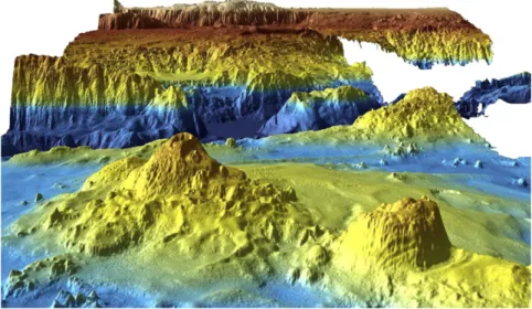
Much of the ocean-bottom topography has been de-scribed, but many details remain uncertain (e.g.,Wessel et al. 2010). Very small-scale topography, presumed to be of importance in oceanic boundary layer physics, remains unknown, and determinable at present only with the limited and expensive shipboard multibeam surveys (seeFIG. 7-9).
As new instrumentation gradually evolved from the 1970s onward (self-contained moored instruments op-erating successfully for months and years, neutrally buoyant floats tracked in a variety of ways, rapid chemical analysis methods, sea surface temperature pictures from the new satellites, etc.), the attention of
much of the seagoing and theoretical communities turned toward the problems of understanding the newly available, if fragmentary, time series. In the background was the knowledge of much of the community of the importance of large-scale meteorological patterns known as weather, and in particular the book byStarr (1968)and the preceding papers. Some of Starr’s students (e.g.,
Webster 1961) had already tried employing limited ocean data in meteorological analogies.
In what became known as the International Decade of Ocean Exploration (IDOE; seeLambert 2000), largely funded in the United States by the National Science Foundation and the Office of Naval Research, much of the oceanographic community focused for the first time on documenting the time variability in the hope of un-derstanding those elements of the ocean that were not in steady state.
A convenient breakdown can be obtained from the various physically oriented IDOE elements: the Mid-Ocean Dynamics Experiment (MODE), POLY-GON1MODE (POLYMODE; the U.S.–Soviet follow-on to ‘‘POLYGON’’ and MODE), North Pacific Ex-periment (NORPAX), International Southern Ocean Studies (ISOS), Climate Long-range Investigation, Map-ping, and Prediction Study (CLIMAP), and Coastal Up-welling Ecosystems Analysis (CUEA). MODE (see
MODE Group 1978) was an Anglo–U.S. collaboration in the western Atlantic south of Bermuda involving moored current meters, temperature–pressure recorders, bottom pressure sensors, Swallow floats, and SOFAR floats.
Figure 7-10shows an initial sketch by H. Stommel of what FIG. 7-9. Diamatina Escarpment in the Indian Ocean; it is about 100 km across. The largest
feature is about 1.5 km high, with a vertical exaggeration of 3 in the scale. Data were obtained in support of the search for the missing Malaysian Airlines flight MH370 aircraft. [Source: From
Picard et al. (2017, their title figure),Ó Kim Picard, Brendan Brooke, and Millard F. Coffin;
eventually became MODE.10 Despite some instrumental problems (the new U.S. current meters failed after approximately a month), the ‘‘experiment’’11showed beyond doubt the existence of an intense ‘‘mesoscale’’ eddy field involving baroclinic motions related to the baroclinic radii of about 35 km and smaller, as well as barotropic motions on a much larger scale. In ocean-ography, the expression mesoscale describes the spa-tial scale that is intermediate between the large-scale ocean circulation and the internal wave field and is thus very different from its meteorological usage (which is closer to the ocean ‘‘submesoscale’’). A better de-scriptor is ‘‘balanced’’ or ‘‘geostrophic’’ eddies, as in the meteorological ‘‘synoptic scale.’’ [The reader is cautioned
that an important fraction of the observed low-frequency oceanic motion is better characterized as a stochastic wave field—internal waves, Rossby waves, etc.—and is at least quasi linear, with a different physics from the vor-texlike behavior of the mesoscale eddies. Most of the kinetic energy in the ocean does, however, appear to be in the balanced eddies (Ferrari and Wunsch 2009)]. Un-derstanding whether the MODE area and its physics were typical of the ocean as a whole then became the focus of a large and still-continuing effort with in situ instruments, satellites, and numerical models.
Following MODE and a number of field programs intended to understand 1) the distribution of eddy en-ergy in the ocean as a whole and 2) the consequences for the general circulation of eddies, a very large effort, which continues today, has been directed at the eddy field and now extending into the submesoscale (i.e., scales between 100 m and 10 km where geostrophic balance no longer holds but rotation and stratification remain important). Exploration of the global field by moorings and floats was, and still is, a slow and painful process that was made doubly difficult by the short FIG. 7-10. A first sketch by H. Stommel (1969, personal communication) of what became the Mid-Ocean
Dy-namics Experiment as described in a letter directed to the Massachusetts Institute of Technology Lincoln Labo-ratory, 11 August 1969. What he called ‘‘System A’’ was an array of 121 ocean-bottom pressure gauges; System B was a set of moored hydrophones to track what were called SOFAR floats; System C was to be the floats themselves (500–1000); System D was described as a numerical model primarily for predicting float positions so that their distribution could be modified by an attending ship; System E (not shown) was to be a moored current-meter array; System F was the suite of theoretical/dynamical studies to be carried out with the observations. The actual ex-periment differed in many ways from this preliminary sketch, but the concept was implemented (although not by Lincoln Laboratories).
10From a letter addressed to the Massachusetts Institute of
Technology Lincoln Laboratory (unpublished document, 11 August 1969).
11Physical oceanographers rarely do ‘‘experiments’’ [the
pur-poseful tracer work ofLedwell et al. (1993)and later is the major exception], but the label has stuck to what are more properly called field observations.
spatial coherence scales of eddies, and the long-measuring times required to obtain a meaningful picture. The first true (nearly) global view became possible with the flight of the high-accuracy TOPEX/Poseidon12 altimeter in 1992 and successor satellite missions. Although limited to measurements of the sea surface pressure (elevation), it became obvious that eddies exist everywhere, with an enormous range in associated kinetic energy (Fig. 7-11). The spatial variation of kinetic energy by more than two orders of magnitude presents important and in-teresting obstacles to simple understanding of the influ-ence on the general circulation of the time-dependent components.
In association with the field programs, the first fine resolution (grid size ,100 km) numerical models of ocean circulation were developed to examine the role of mesoscale eddies in the oceanic general circulation [see the review byHolland et al. (1983)]. Although idealized, the models confirmed that the steady solutions of the ocean circulation derived over the previous decades were hydrodynamically unstable and gave rise to a rich time-dependent eddy field. Furthermore, the eddy fields interacted actively with the mean flow, substantially affecting the time-averaged circulation.
a. Observing systems
As the somewhat unpalatable truth that the ocean was constantly changing with time became evident, and as concern about understanding of how the ocean influ-enced climate grew into a public problem, efforts were undertaken to develop observational systems capable of depicting the global, three-dimensional ocean circula-tion. The central effort, running from approximately 1992 to 1997, was the World Ocean Circulation Exper-iment (WOCE) producing the first global datasets, models, and supporting theory. This effort and its out-comes are described in chapters inJochum and Murtugudde (2006), and inSiedler et al. (2001,2013). Legacies of this program and its successors include the ongoing satellite altimetry observations, satellite scatterometry and grav-ity measurements, the Argo float program, and continu-ing ship-based hydrographic and biogeochemical data acquisition.
Having to grapple with a global turbulent fluid, with most of its kinetic energy in elements at 100-km spatial scales and smaller, radically changed the nature of observational oceanography. The subsequent cultural change in the science of physical oceanography requires
its own history. We note only that the era of the au-tonomous seagoing chief scientist, in control of a sin-gle ship staffed by his own group and colleagues, came to be replaced in many instances by large, highly or-ganized international groups, involvement of space and other government agencies, continual meetings, and corresponding bureaucratic overheads. As might be expected, for many in the traditional oceano-graphic community the changes were painful ones (sometimes expressed as ‘‘we’re becoming too much like meteorology’’).
b. The turbulent ocean
A formal theory of turbulence had emerged in the 1930s from G. I. Taylor, a prominent practitioner of GFD.Taylor (1935)introduced the concept of homogeneous– isotropic turbulence (turbulence in the absence of any large-scale mean flow or confining boundaries), a con-cept that became the focus of most theoretical re-search. Kolmogorov (1941) showed that in three dimensions homogeneous–isotropic turbulence tends to transfer energy from large to small scales. [The book by Batchelor (1953) provides a review of these early results.] Subsequently,Kraichnan (1967)demonstrated that in two dimensions the opposite happens and en-ergy is transferred to large scales.Charney (1971) re-alized that the strong rotation and stratification at the mesoscale acts to suppress vertical motions and thus makes ocean turbulence essentially two dimensional at those scales.
A large literature developed on both two-dimensional and mesoscale turbulence, because the inverse energy cascade raised the possibility that turbulence sponta-neously generated and interacted with large-scale flows. Problematically the emphasis on homogeneous– isotropic turbulence, however, eliminated at the outset any large-scale flow and shifted the focus of turbulence research away from the oceanographically relevant question of how mesoscale turbulence affected the large-scale circulation. A theory of eddy–mean flow in-teractions was not developed for another 30 years, until the work of Bretherton (1969a,b) and meteorologists
Eliassen and Palm (1961)andAndrews and McIntyre (1976).
The role of microscale (less than 10 m) turbulence in maintaining the deep stratification and ocean circulation was recognized in the 1960s and is reviewed below (e.g.,
Munk 1966.) A full appreciation of the role of geo-strophic turbulence on the ocean circulation lagged behind. Even after MODE and the subsequent field programs universally found vigorous geostrophic eddies with scales on the order of 100 km, theories of the large-scale circulation largely ignored this time dependence, 12OceanTopography Experiment/Premier Observatoire Spatial
Étude Intensive Dynamique Ocean et Nivosphere [sic], or Posi-tioning Ocean Solid Earth Ice Dynamics Orbiting Navigator.
primarily for want of an adequate theoretical framework for its inclusion and the lack of global measurements.
That the ocean, like the atmosphere, could be un-stable in baroclinic, barotropic, and mixed forms had been recognized very early.Pedlosky (1964)specifically applied much of the atmospheric theory [Charney (1947),
Eady (1949), and subsequent work] to the oceanic case. Theories of the interactions between mesoscale turbu-lence and the large-scale circulation did not take center stage until the 1980s in theories for the midlatitude cir-culation (Rhines and Young 1982;Young and Rhines 1982) and the 1990s in studies of the Southern Ocean FIG. 7-11. (a) RMS surface elevation (cm) from four years of TOPEX/Poseidon data and (b) the corresponding
kinetic energy (cm2s22) from altimeter measurements (Wunsch and Stammer 1998). The most striking result is the very great spatial inhomogeneity present—in contrast to atmospheric behavior.
(Johnson and Bryden 1989;Gnanadesikan 1999;Marshall and Radko 2003).
Altimetric measurements, beginning in the 1980s, showed that ocean eddies with scales slightly larger than the first deformation radius dominate the ocean eddy kinetic energy globally (Stammer 1997) but with huge spatial inhomogeneity in levels of kinetic energy and spectral distributions (Fig. 7-12), and under-standing their role became a central activity, including the rationalization of the various power laws in this figure. The volume edited byHecht and Hasumi (2008)
and Vallis (2017) review the subject to their corre-sponding dates.
Much of the impetus in this area was prompted by the failure of climate models to reproduce the ob-served circulation of the Southern Ocean. Their grids were too coarse to resolve turbulent eddies at the mesoscale. Because the effect of generation of meso-scale eddies is to flatten density surfaces without causing any mixing across density surfaces (an aspect not previously fully recognized),Gent and McWilliams (1990)proposed a simple parameterization, whose suc-cess improved the fidelity of climate models (Gent et al. 1995). It led the way to the development of theories of Southern Ocean circulation (Marshall and Speer 2012) and the overturning circulation of the ocean (Gnanadesikan 1999;Wolfe and Cessi 2010;Nikurashin and Vallis 2011).
Attention has shifted more recently to the turbulence that develops at scales below approximately 10 km—the so-called submesoscales (McWilliams 2016). Sea surface temperature maps show a rich web of filaments no more than a kilometer wide (seeFig. 7-13).
Unlike mesoscale turbulence, which is characterized by eddies in geostrophic balance, submesoscale motions become progressively less balanced as the scale diminishes— as a result of a host of ageostrophic instabilities (Boccaletti et al. 2007;Capet et al. 2008;Klein et al. 2008;Thomas et al. 2013). Unlike the mesoscale regime, energy is trans-ferred to smaller scales and exchanged with internal gravity waves, thereby providing a pathway toward energy dissipation (Capet et al. 2008). Both the dy-namics of submesoscale turbulence and their in-teraction with the internal gravity waves field are topics of current research and will likely remain the focus of much theoretical and observational investigation for at least the next few decades.
c. The vertical mixing problem
Although mesoscale eddies dominate the turbulent kinetic energy of the ocean, it was another form of tur-bulence that was first identified as crucial to explain the observed large-scale ocean state. Hydrographic sections showed that the ocean is stratified all the way to the bottom. Stommel and Arons (1960a,b) postulated that the stratification was maintained through diffusion of FIG. 7-12. Estimated power laws of balanced eddy wavenumber spectra (Xu and Fu 2012).
From this result and that inFig. 7-11, one might infer that the ocean has a minimum of about 14 distinct dynamical regimes plus the associated transition regions.
temperature and salinity from the ocean surface. How-ever, molecular processes were too weak to diffuse sig-nificant amounts of heat and salt.
Eckart (1948) had described how ‘‘stirring’’ by tur-bulent flows leads to enhanced ‘‘mixing’’ of tracers like temperature and salinity. Stirring is to be thought of as the tendency of turbulent flows to distort patches of scalar properties into long filaments and threads. Mixing, the ultimate removal of such scalars by mo-lecular diffusion, would be greatly enhanced by the presence of stirring, because of the much-extended boundaries of patches along which molecular-scale derivatives could act effectively. [A pictorial cartoon can be seen in Fig. 7-14 (Welander 1955) for a two-dimensional flow. Three-two-dimensional flows, which can be very complex, tend to have a less effective hori-zontal stirring effect but do operate also in the vertical direction.] Munk (1966) in a much celebrated paper, argued that turbulence associated with breaking in-ternal waves on scales of 1–100 m was the most likely candidate for driving stirring and mixing of heat and salt in the abyss—geostrophic eddies drive motions along density surfaces and therefore do not generate any diapycnal mixing.
Because true fluid mixing occurs on spatial scales that are inaccessible to numerical models, and with the un-derstanding that the stirring-to-mixing mechanisms con-trol the much-larger-scale circulation patterns and properties, much effort has gone into finding ways to ‘‘parame-terize’’ the unresolved scales. Among the earliest such efforts was the employment of so-called eddy or Aus-tausch coefficients that operate mathematically like molecular diffusion but with immensely larger numer-ical diffusion coefficients (Defant 1961).Munk (1966)
used vertical profiles of temperature and salinity and estimated that maintenance of the abyssal stratifica-tion required a vertical eddy diffusivity of 1024m2s21 (memorably 1 in the older cgs system) a value that is 1000 times as large as the molecular diffusivity of temperature and 100 000 times as large as the molecu-lar diffusivity of salinity.
For technical reasons, early attempts at measuring the mixing generated by breaking internal waves were confined to the upper ocean and produced eddy diffu-sivity values that were an order of magnitude smaller than those inferred by Munk (see Gregg 1991). This led to the notion that there was a ‘‘missing mixing’’ problem. However, the missing mixing was found when FIG. 7-13. Snapshot of sea surface temperature from the Moderate Resolution Imaging
Spectroradiometer (MODIS) spacecraft showing the Gulf Stream. Colors represent ‘‘bright-ness temperatures’’ observed at the top of the atmosphere. The intricacies of surface temper-atures and the enormous range of spatial scales are apparent. (Source:https://earthobservatory. nasa.gov/images/1393; the image is provided through the courtesy of Liam Gumley, MODIS Atmosphere Team, University of Wisconsin–Madison Cooperative Institute for Meteorological Satellite Studies.)
the technology was developed to measure mixing in the abyssal ocean— the focus of Munk’s argument [see the reviews byWunsch and Ferrari (2004)andWaterhouse et al. (2014)]. Estimates of the rate at which internal waves are generated and dissipated in the global ocean [Munk and Wunsch (1998) and many subsequent pa-pers] further confirmed that there is no shortage of mixing to maintain the observed stratification. The field has now moved toward estimating the spatial patterns of turbulent mixing with dedicated observations, and more sophisticated schemes are being developed to better capture the ranges of internal waves and associated mixing known to exist in the oceans. In particular, it is now widely accepted that oceanic boundary processes, including sidewalls, and topographic features of all scales and types dominate the mixing process, rather than it being a quasi-uniform open-ocean phenomenon (see
Callies and Ferrari 2018).
6. ENSO and other phenomena
A history of ocean circulation science would be in-complete without mention of El Niño and the coupled atmospheric circulation known as El Niño–Southern Oscillation (ENSO). What was originally regarded as
primarily an oceanic phenomenon of the eastern tropi-cal Pacific Ocean, with implications for Ecuador–Peru rainfall, came in the 1960s (Bjerknes 1969; Wyrtki 1975b) to be recognized as both a global phenomenon and as an outstanding manifestation of ocean–atmosphere coupling. As the societal impacts of ENSO became clear, a major field program [Tropical Ocean and Global Atmo-sphere (TOGA)] emerged. A moored observing system remains in place. Because entire books have been devoted to this phenomenon and its history of discovery (Philander 1990;Sarachik and Cane 2010;Battisti et al. 2019), no more will be said here.
The history of the past 100 years in physical ocean-ography has made it clear that a huge variety of phe-nomena, originally thought of as distinct from the general circulation, have important implications for the latter. These phenomena include ordinary surface gravity waves (which are intermediaries of the transfer of momentum and energy between ocean and atmo-sphere) and internal gravity waves. Great progress has occurred in the study of both of these phenomena since the beginning of the twentieth century. For the surface gravity wave field, see, for example,Komen et al. (1994). For internal gravity waves, which are now recognized as central to oceanic mixing and numerous other processes, the most important conceptual development of the last 100 years was the proposal by Garrett and Munk (1972; re-viewed byMunk 1981) that a quasi-universal, broadband spectrum existed in the oceans. Thousands of papers have been written on this subject in the intervening years, and the implications of the internal wave field, in all its gen-eralities, are still not entirely understood.
7. Numerical models
Numerical modeling of the general ocean circulation began early in the postwar computer revolution. Nota-ble early examples were Bryan (1963) and Veronis (1963). As computer power grew, and with the impetus from MODE and other time-dependent observations, early attempts [e.g.,Holland (1978), shown inFig. 7-15] were made to obtain resolution adequate in regional models to permit the spontaneous formation of bal-anced eddies in the model.
Present-day ocean-only global capabilities are best seen intuitively in various animations posted on the Internet (e.g.,
https://www.youtube.com/watch?v5CCmTY0PKGDs), al-though even these complex flows still have at best a spatial resolution insufficient to resolve all important processes. A number of attempts have been made at quantitative description of the space–time complexities in wavenumber–frequency space [e.g., Wortham and Wunsch (2014)and the references therein].
FIG. 7-14. Sketch (Welander 1955) showing the effects of ‘‘stir-ring’’ of a two-dimensional flow on small regions of dyed fluid. Dye is carried into long streaks of greatly extended boundaries where very small scale (molecular) mixing processes can dominate. (Ó 1955 Pierre Welander, published by Taylor and Francis Group LLC underCC BY 4.0license.)
Ocean models, typically with grossly reduced spatial resolution have, under the growing impetus of interest in climate change, been coupled to atmospheric models. Such coupled models (treated elsewhere in this volume) originated with one-layer ‘‘swamp’’ oceans with no dynamics. Bryan et al. (1975) pioneered the representation of more realistic ocean behavior in coupled systems.
a. The resolution problem
With the growing interest in the effects of the bal-anced eddy field, the question of model resolution has tended to focus strongly on the need to realistically
resolve both it and the even smaller submesoscale with Rossby numbers of order 1. Note, however, that many features of the quasi-steady circulation, especially the eastern and western boundary currents, require resolu-tion equal to or exceeding that of the eddy field. These currents are very important in meridional property transports of heat, freshwater, carbon, and so on, but parameterization of unresolved transports has not been examined.Figure 7-16shows the Gulf Stream temper-ature structure in the WOCE line at 678W for the top 500 m (Koltermann et al. 2011). The very warmest water has the highest from-west-to-east u velocity here, and its structures, both vertically and horizontally, are impor-tant in computing second-order productshuCi for any property C—including temperature and salinity. Apart from the features occurring at and below distances of about 18 of latitude, like the submesoscale, the vertical structure requires resolution of baroclinic Rossby radii much higher than the first one.
For the most part, ocean and climate modelers have sidestepped the traditional computational requirement of demonstrating numerical convergence of their codes, primarily because new physics emerges every time the resolution is increased. Experiments with regional, but very high resolution, models suggest, for exanple, that, in the vicinity of the Gulf Stream (and other currents), latitude and longitude resolution nearing 1/508 (2 km) is required (Lévy et al. 2010). In the meantime, the com-putational load has dictated the use of lower-resolution models of unknown skill—models sometimes labeled as ‘‘intermediate complexity’’ and other euphemisms. When run for long periods, the accuracy and precision in the presence of systematic and stochastic errors in under-resolved models must be understood.
b. State estimation/data assimilation
The meteorological community, beginning in the early 1950s (Kalnay 2002), pioneered the combination of ob-servational data with system dynamics encompassed in the numerical equations of general circulation models [numerical weather prediction (NWP) models]. Almost all of this work was directed at the urgent problem of weather forecasting and came to be known as ‘‘data similation.’’ In the wider field of control theory, data as-similation is a subset of much more general problems of model–data combinations (seeBrogan 1990). In partic-ular, it is the subset directed at prediction—commonly for days to a couple of weeks.
When, in much more recent years, oceanographers did acquire near-global, four-dimensional (in space and time) datasets, the question arose as to how to make ‘‘best estimates’’ of the ocean using as much of the data as possible and the most skillful GCMs. The well-FIG. 7-15. An early attempt at showing an instantaneous flow
field in an ocean numerical model with resolved eddies. Shown are a snapshot of the streamfunctions in the (top) upper and (bottom) lower layers of a two-layer model (Holland 1978). Note the very limited geographical area.